Accurate robot simulation

(1)

This is a repository copy of

Accurate robot simulation

_.

White Rose Research Online URL for this paper:

http://eprints.whiterose.ac.uk/74645/

Monograph:

Nehmzow, U., Kerr, D. and Billings, S.A. (2009) Accurate robot simulation. Research

Report. ACSE Research Report no. 992 . Automatic Control and Systems Engineering,

University of Sheffield

[email protected] https://eprints.whiterose.ac.uk/ Reuse

Unless indicated otherwise, fulltext items are protected by copyright with all rights reserved. The copyright exception in section 29 of the Copyright, Designs and Patents Act 1988 allows the making of a single copy solely for the purpose of non-commercial research or private study within the limits of fair dealing. The publisher or other rights-holder may allow further reproduction and re-use of this version - refer to the White Rose Research Online record for this item. Where records identify the publisher as the copyright holder, users can verify any specific terms of use on the publisher’s website.

Takedown

If you consider content in White Rose Research Online to be in breach of UK law, please notify us by

(2)

Accurate Robot Simulation

Ulrich Nehmzow

1

_{Dermot Kerr}

1

_{S A Billings}

2

1_{Intelligent Systems Research Centre, University of Ulster, Londonderry, BT48 7JL, UK}

2_{Department of Automatic Control and Systems Engineering, University of Sheffield, Sheffield, S1 3JD, UK}

Abstract

Robot simulators are valuable tools for re-searchers to develop control code in a fast and efficient manner without spending time setting up physical experiments. Most simulators, however, do not model the real world accurately. As a con-sequence, when a program is run on a real robot it may behave differently from when run in simula-tion. In this paper we present a method of devel-oping a robot simulator that models the operation of a real robot in a real environment accurately, using real robot data and system identification to construct the simulator’s model.

1. Introduction

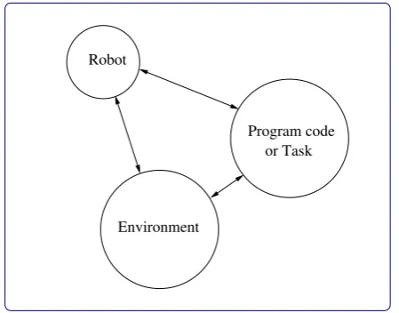
When considering the behaviour of a robot, there are three components that influence the system: (i) robot hardware, (ii) the program being executed, and (iii) the robot’s environment. Thus, the interaction of these three components, as illustrated in Figure 1, constitutes a highly complex system from which the overall robot behaviour emerges.

Environment

[image:2.595.64.289.481.657.2]

or Task Program code Robot

Figure 1: Overall robot behaviour emerges from the

interaction between robot, task and environment

The common procedure to develop a control program is for the robot programmer to write the program “as best as possible” whilst considering the desired task.

However, it is unlikely that the desired behaviour will be obtained immediately, as the robot programmer has to make (often idealistic, simplifying) assumptions about the robot’s hardware and properties of the environment. Typically, the desired robot behaviour is eventually ob-tained by a process of iterative refinement of the control program.

Robot simulators are therefore useful for researchers to develop and test new controllers. Simulators can save time and effort by concentrating on the development of the controller, rather than spending time on i) setting-up real world experiments and ii) waiting for experiments to complete, as using a simulator allows the researcher to run experiments faster than real-time. Additionally, simulators are the only way to provide a consistent rep-etition of experiments.

Traditional trial-and-error-based approaches of pro-gramming robots lack a rigorous design methodology, they are costly, time consuming and error prone. In this paper we present an alternative, describing a de-sign method for a mobile robot simulator that accurately models and simulates a physical robot’s interaction with its environment, performing a particular task.

The overall aim of this research is theautomatic

gen-eration of control code, without the need for an experi-enced robot engineer to perform iterative refinement and trial-and-error procedures. As a step towards this goal, in this paper we present our experiments to create ac-curate robot simulators that make precise predictions of robot sensor measurements based on the robot’s position in the environment.

1.1 Motivation

A number of existing robot simulators exist within the robotics community, some are generic such as Player-Stage (Gerkey et al., 2003) and Webots (Michel, 2004), others are platform dependent such as the Kephera sim-ulator (Michel, 1996). The ability of these robot simu-lators to predict accurately depends on three models: i) the robot model, ii) the task model, and iii) the envi-ronment model. The envienvi-ronment model provides the robot’s sensory perception based on the robot’s posi-tion and orientaposi-tion and is of the main interest to this

work. This model is dependent on the structure of

(3)

environment is composed of. However, being generic, they are based on general assumptions of environment properties and fail to model extreme perceptions such as specular reflections. As argued in (Lee et al., 1998, Kyriacou et al., 2008) we believe that faithful simulation

is only obtainable when specific environmental

scenar-ios are modelled using data obtained fromreal

environ-ments.

1.1.1 Possible Approaches

In the simulator developed by Lund and

Miglino (Lund and Miglino, 1996), logged data is

stored in a lookup table and values are interpolated to predict sensory perception at unvisited locations. In (Lee et al., 1998) a neural network is used to model the input-output relationships between robot location

and sensor perception. This approach works well,

however, neural networks produce an opaque model that cannot be used to investigate the characteristics of the inputs and outputs further (such as stability analysis, sensitivity of the behaviour to particular sensor (Saltelli et al., 2000) or environmental features, sensor redundancy etc). Additionally, the structure of a neural network does not allow straightforward comparison between different models. Here, we therefore propose a transparent modelling method, which is most closely related to the work presented in (Kyriacou et al., 2008). In Kyriacou’s paper, a robot simulator is built using mathematical models representing the sensor perception based on the robots location. Our work differs from (Kyriacou et al., 2008), however, in that we create parsi-monious sensor models based on the robot’s orientation

ϕ, rather than having many separate sensor models for

each (x, y) location in the robot’s environment.

2. Modelling Method

We propose the use of system identification, as used in (Kyriacou et al., 2008), to develop accurate robot simulation. We determine the relevant input-output pa-rameters of the sensor simulation process — the accurate simulation of laser perception based on a robot’s posi-tion, and validate the resulting laser perception against the robot’s real laser perception along a (separately logged) validation path.

In this work we adopt the use of system identification, rather than alternative modelling approaches such as ar-tificial neural networks or lookup tables, because it offers numerous benefits: the obtained models are compact, as they consist of a single polynomial with a small num-ber of terms; and the obtained models are transparent and can be examined using standard techniques such as sensitivity analysis (Saltelli et al., 2000).

NARMAX (Non-linear Auto-Regressive Moving Av-erage model with eXogenous inputs) is a parameter

es-timation methodology to identify the important model terms and their associated parameters of a non-linear polynomial model of an unknown non-linear dynamic system. The NARMAX methodology breaks the mod-elling problem into the following steps: i) Structure de-tection, ii) parameter estimation, iii) model validation, iv) prediction, and v) analysis. A detailed procedure of these steps is presented in (Chen and Billings, 1989, Billings and Voon, 1986, Korenberg et al., 1988), and details of the application of NARMAX to mobile robot simulation in (Kyriacou et al., 2008).

In this work we obtain a model that relates the robot’s

positional location to its laser perception. The fact

that we obtain the model as a transparent polynomial representation makes the model easily and accurately transferable to any robot platform with the same sen-sor type and configuration. Another benefit of the com-pact mathematical form of the model is that it can be directly implemented in any computer language using

standard mathematical libraries. This minimises the

time to translate programs between robot platforms and languages. Increased execution time and reduced mem-ory requirements are also obtained due to the task code being condensed into a single polynomial with the mod-elling process.

3. Experiments

The experiments in this paper where carried out in the robotics arena of the Intelligent Systems Research Centre in the University of Ulster. The robotics arena measures

100 m2

and is equipped with a powered floor, a Vicon

motion tracking system and a large number of robots. In all the experiments described in this paper we used the

MetralabsSCITOS G5 autonomous robotSwilly, shown

in Figure 2. The robot is equipped with 24 sonar

sen-sors distributed around its circumference and a SICK

laser range finder, which scans the front of the robot ([0◦_,270◦_{]) with a radial resolution of 0.5}◦_{. In our}

exper-iments the laser range finder was configured to scan the front semi-circle of the robot in the range ([0◦_,180◦_]).

3.1 Experimental Set-Up

During the experiments the input from the robot’s laser, position, orientation, transitional and rotational veloci-ties were logged every 250 ms. In addition, the robot’s

actual x, y, zpositions obtained from the Vicon motion

tracking system are logged simultaneously at 50 Hz, at this speed the positional error was less than 1 mm.

(4)

[image:4.595.323.551.68.238.2] [image:4.595.92.260.70.274.2]

Figure 2: Swilly, the Metralabs SCITOS G5 mobile robot used in the experiments

Figure 3: Robot arena setup

3.1.1 The

Sensorgraph

In our experiments we first construct what we term a

sensorgraph — a detailed log of sensor perceptions ob-tained in the environment — by using the robot to collect data from the environment that is being modelled. The data that is collected during this process are the robot’s position, orientation, laser perception and ground truth

position (obtained using theVicon motion tracking

sys-tem). A random walk obstacle avoidance program

us-ing the laser sensor is run on Swilly, involving obstacle

avoidance and random rotations to the robot’s move-ment at predefined intervals. The basis of introducing the random rotations is to try and ensure that the robot explores as much of the environment as possible at dif-ferent orientations. In Figure 4 we show the actual

posi-tions where Swilly logged data, over 1400 data samples

in these experiments.

It is important that the robot has logged adequate data throughout this data collection stage, as the

ob-−200 −100 0 100 200

−100 −50 0 50 100 150 200 250

Vicon x−axis displacement [cm]

[image:4.595.91.264.319.462.2]

Vicon y−axis displacement [cm]

Figure 4: Data sampling points

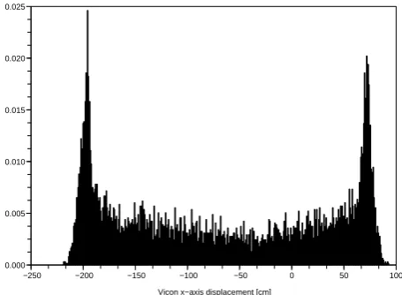
tained model’s accuracy will depend on the data con-tained in the sensorgraph. Therefore, to ensure that we have a good distribution of values we computed

his-tograms for the robot’s position obtained using theVicon

tracking system along thex-axis andy-axis (Figures 5

and 6). Although the histograms show a denser

distri-bution of thesensorgraph data at the arena edges, they

show that all possiblyxandylocations are equally often

visited (uniform distribution) — a desirable property for a sensorgraph.

−250 −200 −150 −100 −50 0 50 100 0.000

0.005 0.010 0.015 0.020 0.025

Figure 5: Histogram of visitedxpositions

It is also important to consider the robot’s heading, because the modelling process needs to consider all pos-sible orientations of the robot. In Figure 7 we illustrate the histogram representing the rotational angles where the robot has logged data as contained in the sensor-graph, again a good almost-uniform distribution.

After the data was collected we median-filtered the

laser data over 30◦_{segments. Thus, rather than 360 laser}

readings ([0◦_,180◦_] ×_0.5◦ _{resolution), we then used the}

[image:4.595.321.549.414.581.2]

(5)

−250 −200 −150 −100 −50 0 50 100 150 200 0.000

0.002 0.004 0.006 0.008 0.010 0.012 0.014

[image:5.595.62.289.68.236.2]

Vicon y−axiz displacement [cm]

Figure 6: Histogram of visitedy positions

−200 −150 −100 −50 0 50 100 150 200 0.000

0.001 0.002 0.003 0.004 0.005 0.006

[image:5.595.63.288.264.438.2]

phi

Figure 7: Histogram of headings ϕ at data-logging

points

L15=median[0◦,30◦] L45=median[30◦,60◦] L75=median[60◦_,₉₀◦_]

L105=median[90◦,120◦] L135=median[120◦_,₁₅₀◦_{] and}

L165=median[150◦,180◦]

as input to our modelling process.

3.1.2 Models For Different

ϕ

After logging the sensorgraph data, it is required to com-pute a model which predicts the robot’s sensor percep-tion, given the robot’s position and orientation. When computing this model we need to consider all the possible (x,y) positional locations the robot may visit, as well as

the robots orientationϕat these positions. The

dimen-sionality of this space is very high, and in order to

man-age the task of constructing a model we have restricted

the number of models to only 12 models, modelling 30◦

segments, thus covering the entire 360◦ _{range of}

possi-ble robot headings with 12 models. Put differently, we

constructed 12 models, one for each 30◦_{segment, of the}

form Lk =f(x, y)∀ϕ = k, where Lk is a model of the

laser reading when the robot assumes a headingϕof k

degrees.

3.1.3 Validation Trajectories

To validate the robot’s predicted sensor perceptions

based on the robot’s position (x, y) and orientation ϕ,

a number of independent validation runs were logged by manually driving the robot along a novel path immedi-ately after the logging of the sensorgraph. During these validation runs the robot’s position (obtained using the

Vicontracking system) and laser perception were logged. In Figure 8 and Figure 9 we show the trajectory of two validation runs, along with the original sampling points used to obtain the sensorgraph.

−200 −100 0 100 200

−100 −50 0 50 100 150 200 250

[image:5.595.324.550.331.501.2]

Figure 8: Validation trajectory 1

−200 −100 0 100 200

−100 −50 0 50 100 150 200 250

[image:5.595.325.549.543.714.2]

(6)

These validation runs allow us to compare, measure and validate how the actual real sensor perception com-pares with the model’s predicted values along a new tra-jectory.

3.2 Initial Results

After collection of the data in the sensorgraph we use the NARMAX system identification procedure to esti-mate the robot’s laser perception as a function of the

the robot’s location, obtained using the Vicon tracking

system and using the logged training data. As described earlier, 12 polynomials were obtained in total, express-ing the laser perception of the robot as a function of

the robots location and heading to the nearest 30◦_{. The}

models were chosen to be of fourth degree and no regres-sion was used in the inputs and outputs.

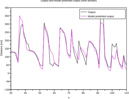
For example, for ϕ =−₇₅◦±₁₅◦ _{and laser segment}

L75 this resulted in a NARMAX polynomial structure

containing 9 terms

Lp75/cm= +223.74

+ 1.47∗_x + 0.68∗_y

−₀_.₀₀₂∗_x2

−₀_.₀₀₁∗_y2

−₀_.₀₀₀₁∗_x3

−₀_._00000036∗_x4

+ 0.00000006∗_y4

+ 0.000012∗_y∗_y2_.

The difference between model prediction and true value is shown in Figure 10.

30 40 50 60 70 80 90 100 110 −100

−50 0 50 100 150 200 250 300 350 400

Output and Model predicted output (time domain)

n

Distance [cm]

Output Model predicted output

Figure 10: Actual and predicted laser readings along

validation trajectory 1

For ϕ =−₁₆₅◦±₁₅◦ _{and laser segment} _L₇₅ _this

re-sulted in a NARMAX polynomial structure containing 4 terms

Lp75/cm= +234.84

+ 0.85∗_x + 0.30∗_y + 0.0014∗_x∗_y,

the model validation is illustrated in Figure 11.

190 200 210 220 230 240 250 260 270 280 290 0

50 100 150 200 250 300 350

Output and Model predicted output (time domain)

n

Distance [cm]

[image:6.595.324.548.217.388.2]

Output Model predicted output

Figure 11:Actual and predicted laser readings along

validation trajectory 2

In a similar manner we computed all 12 models for the

range of orientationsϕand for each laser segment.

3.2.1 Assessment 1

To assess the performance of the obtained polynomial models we used the validation trajectory 1 (Figure 8). In Figure 12 we plot the predicted laser values for the

segment ˜L75 against the actual laser valuesL75.

In Figure 13 we plot the predicted laser values for the

segmentL105˜ against the actual laser valuesL105.

Mean error and standard error for validation trajec-tory 1 are given in Table 1.

3.2.2 Assessment 2

We also assessed the performance of the obtained poly-nomial models for a more complex non-linear trajectory, such as the one given in validation trajectory 2 (Fig-ure 9). Fig(Fig-ure 14 shows the predicted laser values for

the segment ˜L75against the actually logged laser values

[image:6.595.63.289.532.705.2]

L75.

Figure 15 shows the predicted laser values for the seg-mentL105˜ against the actual laser valuesL105.

(7)

0 10 20 30 40 50 60 70 80 0

50 100 150 200 250 300 350

Time [250ms]

Laser range [cm]

[image:7.595.65.289.89.259.2]

Logged laser Predicted laser

Figure 12: Predicted laserL˜75 values against actual

logged laserL75 values for validation trajectory 1

0 10 20 30 40 50 60 70 80

0 50 100 150 200 250 300 350

Time [250ms]

Laser range [cm]

[image:7.595.323.551.90.257.2]

Figure 13:Predicted laserL105˜ values against actual

Table 1: Absolute Mean error and Standard error in

centimetres for validation trajectory 1

Laser Mean and Standard error [cm]

˜

L15 60±5

˜

L45 53±₅

˜

L75 31±₄

˜

L105 17±4

˜

L135 21±2

˜

L165 20±₂

0 50 100 150

0 50 100 150 200 250 300 350 400 450 500

Time [250ms]

Laser range [cm]

[image:7.595.64.289.335.505.2]

Figure 14: Predicted laser L˜75 values against actual

0 50 100 150

0 50 100 150 200 250 300 350 400

Time [250ms]

Laser range [cm]

Figure 15:Predicted laserL˜105 values against actual

logged laserL105values for validation trajectory 2

Table 2: Absolute Mean error and Standard error in

centimetres for validation trajectory 2

Laser Mean and Standard error [cm]

˜

L15 62±₃

˜

L45 46±4

˜

L75 66±4

˜

L105 39±3

˜

L135 29±₄

˜

[image:7.595.323.551.335.503.2] [image:7.595.345.528.614.715.2] [image:7.595.84.265.617.713.2]

(8)

Further Statistical Evaluations _{We also}

per-formed numerical tests to determine the performance of the simulator for this second validation trajec-tory, and compared the error of the simulator model against the error of a “random guess” simulator that generates random predictions from the range of

valid laser measurements. The Mann-Whitney U

-test (Snedecor and Cochran, 1989, Barnard et al., 1993) was performed on both pairs of distributions in order to check if they are significantly different or not. Both tests indicated that the distributions are different at the 5% significance level as illustrated in Figure 16 for the

laser segment ˜L75and in Figure 17 for the laser segment

˜

L105. In other words, the obtained model performs

sig-nificantly better than a random guess.

Frequency

Error [cm]

Frequency

Error [cm] 0 50 100 150 200 250 300 350 400 450 500 0

5 10 15 20 25 30 35

0 50 100 150 200 250 300 350 400

0 2 4 6 8 10 12 14

Error distribution of random guess prediction of laser range Error distribution of model−predicted laser range

Figure 16: U-statistic illustrating comparison of

pre-dicted laser error with random guess error for laserL75

[image:8.595.323.548.70.284.2]

The Spearman rank correlation coefficients between actual laser perception and predicted laser perception are given in Table 3, they are all significant (p <0.05).

Table 3: Spearman rank correlation coefficients

be-tween predicted and actual laser readings for val-idation trajectory 2. All correlations are statisti-cally significant (p <0.05).

Laser segment SR

1 0.7264930

2 0.3045180

3 0.9775737

4 0.9275737

5 0.7720901

6 0.7360612

Frequency

Error [cm]

Frequency

Error [cm]

0 50 100 150 200 250 300 350 400

0 2 4 6 8 10 12 14

Error distribution of random−guess prediction of laser range

0 50 100 150 200 250 300 350 400

0 5 10 15 20 25 30 35 40

[image:8.595.60.290.265.477.2]

Error distribution of model−predicted laser range

Figure 17: U-statistic illustrating comparison of

pre-dicted laser error with random guess error for laserL105

4. Summary And Conclusions

4.1 Summary

In this paper we have presented an approach to model a robot’s laser perception based on position and orien-tation, using the NARMAX model estimation method-ology. The mobile robot is used to explore the envi-ronment whilst logging sensor perception and its actual position. This data is then used to construct models that predict the robot’s perception based on its position and orientation. To evaluate the performance accuracy of the obtained models we compared the robot’s real sensor perception along two independent validation runs with the sensor perception predicted by our model.

4.2 Conclusions

We have shown how to model a robot’s laser perception as a function of its position, using compact polynomial models, and how the NARMAX modelling approach can be used to produce transparent mathematical functions that can be related directly to the modelling task.

This method of simulating the robot’s perception has a number of important benefits. Simulator development is fast and the obtained model is very compact. The model is transparent, i.e. represented as a polynomial function that can be analysed mathematically.

4.3 Future Work

(9)

code. The goal of this research is to have a robot observe a human performing a task, and for the robot to gener-ate control code automatically from this observation to perform the same task. The experiments presented here illustrate that it is possible to create a model of sensor perception as a function of the robot’s position within the environment. The next stage in this research is to

model a human task, using theVICON tracking system.

Using the demonstrator’s trajectory we will estimate the robot’s perception at these positions, using the method described in this paper, to create a new model that mim-ics the task performed by the human demonstrator.

References

Barnard, C., Gilbert, F., and McGregor, P. (1993).
Ask-ing questions in biology. Longman, Harlow, UK.
Billings, S. and Voon, W. S. F. (1986). Correlation
based model validity tests for non-linear models.
In-ternational Journal of Control, 44:235–244.
Chen, S. and Billings, S. A. (1989). Representations
of non-linear systems: The narmax model. Int. J.
Control, 49:1013–1032.
Gerkey, B., R.Vaughan, and Howard, A. (2003). The player/stage project: Tools for multi-robot and
dis-tributed sensor systems. In Proceedings of the
In-ternational Conference on Advanced Robotics.
Korenberg, M., Billings, S., Liu, Y., and McIlroy, P. (1988). Orthogonal paramter estimation for
non-linear stochastic systems. Int. J. Control, 48:193–
210.
Kyriacou, T., Nehmzow, U., Iglesias, R., and Billings, S. A. (2008). Accurate robot simulation through
system identification. Robotics and Autonomous
Systems, 56:1082–1093.
Lee, T., Nehmzow, U., and Hubbold, R. J. (1998). Mo-bile robot simulation by means of acquired neural
network models. InESM, pages 465–469.
Lund, H. H. and Miglino, O. (1996). From simulated
to real robots. In Proceedings IEEE International
Conference on Evolutionary Computation.
Michel, O. (1996). Kephera simulator version 2.0 user manual.
Michel, O. (2004). Webots: Professional mobile robot
simulation. Advanced Robotic Systems, 1:40–43.
Saltelli, A., Chan, K., and Scott, E. M. (2000).
Sensi-tivity analysis. Wiley.
Snedecor, G. W. and Cochran, W. G. (1989).Statistical