EXTREMELY SHEAR-THINNING FLUID
by G. RICHARDSON†and J. R. KING(Section of Theoretical Mechanics, University of Nottingham, Nottingham NG7 2RD)
[Received 2 August 2006. Revise 16 January 2007]
Summary
We consider a steady flow driven by pushing a finger of gas into a highly shear-thinning power-law fluid, with exponent n, in a Hele-Shaw channel. We formulate the problem in terms of the streamfunctionψ, which satisfies the p-Laplacian equation∇ ·(|∇ψ|p−2∇ψ) = 0 (with p = (n +1)/n), and investigate travelling wave solutions in the large-n (extreme shear-thinning) limit. We take a Legendre transform of the free-boundary problem forψ, which reduces it to a linear problem on a fixed domain. The solution to this problem is found by using matched asymptotic expansions and the resulting shape of the finger deduced (being, to leading order, a semi-infinite strip). The nonlinear problem for the streamfunction is also treated using matched asymptotic expansion in the physical plane. The finger-width selection problem is briefly discussed in terms of our results.
1. Introduction
The Saffman–Taylor problem has been the subject of a great deal of interest for nearly fifty years. It was initially posed in order to describe experiments by Saffman and Taylor (1). These involved pushing a finger of air into a Hele-Shaw channel, filled with a Newtonian liquid, under the action of a pressure difference. It was observed that the ratioλof the selected finger width to that of the channel is one-half (except when the injection is very slow). In addition, Saffman and Taylor (1) derived a family of zero surface tension solutions, parametrized byλ, describing the finger shape. Finger-width selection remained unexplained until a numerical calculation of finger shape, in the presence of surface tension, was performed by McLean and Saffman (2). Subsequently asymptotic methods have been used to derive the celebrated resultλ=1/2 in the limit of low surface tension (or high finger velocity) (3 to 5), as well as in limiting cases of other regularizations such as kinetic undercooling (6) (see also (7) for a review of the subject). We stress, however, that there are other circumstances in which the selected finger does not haveλ=1/2 (see (8), in particular), including the near-Newtonian limit of power-law fluids (9, 10).
Hele-Shaw flows of power-law fluids (with general exponent n; see (4) below) have been inves-tigated by Aronsson and Janfalk (11), who obtain similarity solutions describing (i) flow about a corner (ii) doublet flows and (iii) spiral flows. The Hele-Shaw free-boundary problem, describing the motion of an interface between air and fluid, was considered by King (12), who investigated a local problem describing the flow in the vicinity of a corner in the free boundary. In particular, (12) shows that under injection the corner persists for finite time if its angle is less than some critical angle, whereas if it exceeds this angle the corner immediately smooths. Under suction the corner
persists, if its angle is subcritical, until the solution ceases to exist. Saffman–Taylor type problems for power-law fluids have been investigated by Alexandrou and Entov (13), who consider the zero surface tension case, and Ben Amar and Corvera Poir´e (9, 10) who investigate the near-Newtonian limit (|n−1| 1) and postulate that for shear-thinning fluids the selected finger widthλdecreases towards zero as the surface tensionσ tends to zero.
It is the aim of this work to find asymptotic solutions to the Saffman–Taylor problem in which a symmetric finger of air is pushed into a Hele-Shaw channel, filled with a strongly shear-thinning power-law fluid. Such extreme shear-thinning fluid flows give rise to highly-nonlinear elliptic partial differential equations (PDEs) for both the stream functionψand the pressure p, corresponding to the limit n→ ∞in
∇ ·
∇ψ |∇ψ|1−1/n
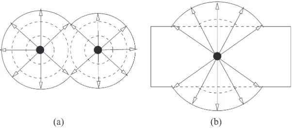
=0, ∇ ·(|∇p|n−1∇p)=0, (1) respectively. In the context of such flows we note that considerable progress has been made, in this limit, on injection problems (whereby fluid is injected into a Hele-Shaw cell at one or more points) by Aronsson and co-workers; see, in particular, (14) which describes how, in the absence of surface tension, the free boundary of the fluid follows the level sets of an interior distance function centred on the injection points. At its most basic level this approach consists in noting that the ‘naive’ limit of the streamfunction problem (1) is the degenerate one
∇ ·
∇ψ |∇ψ|
=0. (2)
This limit problem forψ is parabolic and the associated streamlines (lines on which ψ is con-stant) are, necessarily in the two-dimensional case treated here, straight lines: equation (2) simply states that the level sets ofψhave zero mean curvature. It is informative to compare this with the corresponding limit problem for the pressure equation (1a), namely the eikonal equation
|∇p| =1, (3)
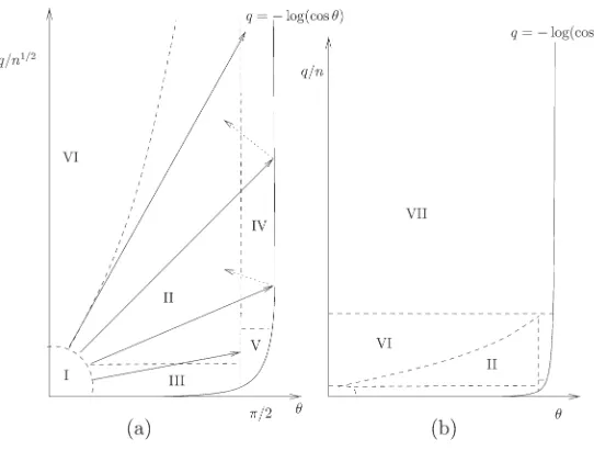
Fig. 1 Injection from (a) two points with no fluid initially present and (b) from a single point into an initially rectangular domain. Here dashed lines show previous positions of the fluid domain, while the solid one shows the present position. Lines with arrows show the asymptotic streamlines
film Hele-Shaw flows of extremely shear-thinning fluids (with applications to compression mould-ing) have been investigated by Aronsson and Evans (18) and Bergwall (19). The extreme shear-thinning limit of power-law fluid flows has also been considered, outside the Hele-Shaw context, by Brewster et al. (20) and Chapman et al. (21), who observe that even simple flows, such as Jeffrey– Hamel flows in a wedge, exhibit a rich asymptotic structure. The time-dependent version of the large-n limit of (1b) has also been considered in the context of Bean model, which models the motion of superconducting vortices in so-called ‘dirty’ superconductors; see, for example, (22).
Little, however, is known about the corresponding Hele-Shaw suction problem other than that it is ill-posed (see, for example, (12)). A number of works consider the Saffman–Taylor problem for power-law fluids in a channel. In (9, 10) a semi-numerical, semi-asymptotic method is used to study the Saffman–Taylor finger selection problem in the limit of n→1 (that is, for a nearly-Newtonian fluid). For O(1)values of the dimensionless surface tension the finger width is little changed from its Newtonian value, but for small surface tension there is a significant decrease in finger width as n increases above unity. Alexandrou and Entov (13) construct symmetric Saffman–Taylor fingers for arbitrary values of the power-law exponent n (and for Bingham fluids) but with zero surface tension (ZST) on the free boundary. In order to do this they apply a linearizing hodograph transformation to the problem, resulting in a linear elliptic PDE on a fixed domain in the hodograph plane that is solved numerically. Although this approach cannot predict finger width, it does predict finger shape and (13, Fig. 3) is suggestive of our results below that in the large-n limit this approaches a semi-infinite strip. Experimental studies of viscous fingering (and of finger-width selection) in non-Newtonian fluids have been conducted by Lindner et al. (23, 24), with the conclusion that narrow fingers are selected in shear-thinning fluids.
2. Problem formulation
The velocity of the fluid w is given in terms of the pressure p by (working throughout in dimension-less terms)
Assuming incompressibility leads to
∇ ·|∇p|n−1∇p
=0.
Alternatively, the problem can be formulated in terms of the stream functionψdefined by w=∂ψ
∂yex− ∂ψ
∂xey. (5)
This leads to following ‘Cauchy–Riemann’ relations between p andψ: ∂p
∂x = − 1 |∇ψ|1−1/n
∂ψ ∂y,
∂p ∂y =
1 |∇ψ|1−1/n
∂ψ ∂x, and hence to
∇ ·
∇ψ |∇ψ|1−1/n
=0; (6)
it is noteworthy that, though they are of different order, equations (2) and (3) can be mapped to each other via
∂p ∂x = −
1 |∇ψ|
∂ψ ∂y,
∂p ∂y =
1 |∇ψ|
∂ψ ∂x.
Without loss of generality we consider the finger to move with unit (dimensionless) velocity in the x-direction. In the case of zero surface tension the boundary conditions on the free boundary∂f
(with outward normal N) are
p|∂f =0, N·w|∂f =ex ·N, (7)
the latter equation corresponding to the kinematic condition in this travelling wave case. We can rewrite these in terms ofψas
∂ψ ∂N
∂f
=0, ∂ψ ∂s
∂f
=ex·N, (8)
where s is arc length along the boundary. In addition, boundary conditions on the edges of the Hele-Shaw cell (namely the impermeable channel walls y= −1 and y=1) must be imposed. Assuming a finger of width 2λ, the flux of fluid through a cross-section of the cell is 2λand we may choose the origin ofψsuch that
ψ|y=1=λ, ψ|y=−1= −λ. (9)
Imposing symmetry about the centreline x =0, so thatψ|y=0=0, integrating (8)2and collating
the equations and boundary conditions forψgives the following closed problem, ifλis specified, which determinesψup to an arbitrary translation in x:
∇ ·
∇ψ |∇ψ|1−1/n
=0, (10)
∂ψ ∂N
∂f
=0, ψ|∂f =y, (11)
ψ∼λy as x→ ∞, (12)
The main aim of this work to find an asymptotic solution to this problem in the highly-nonlinear (strongly shear-thinning) limit n→ ∞.
3. The Legendre transform
In order to analyse (10) to (13) it is helpful first to reformulate them using a Legendre transform. This has the benefit that the transformed variable satisfies a linear problem in a fixed domain. In this context we note, first, that Atkinson and Champion (25), for example, have used this approach to derive exact solutions to equation (1) (although they term this transformation a ‘hodograph trans-form’) and, secondly, that Alexandrou and Entov (13) have instead used a hodograph transform (that is, in the notation below,ψis calculated as a function of a and b); although the latter approach also linearizes the problem, it proves more difficult to invert the solution of the transformed problem to obtain the physical variables. The Legendre transform is accomplished by introducing three new variables
a=ψx, b=ψy, =xψx+yψy−ψ (14)
(henceforth such subscripts denote derivatives). Differentiatingwith respect to x and y and using the fact that ay=bx gives rise, in the usual way, to the inversion formulae
x=a, y=b, ψ =aa+bb−. (15)
The following expressions for the second derivatives ofψcan then be derived by using the chain rule:
ψx x =
bb aabb−ab2
, ψx y = −
ab aabb−ab2
, ψyy=
aa aabb−ab2
.
It is now a simple matter to transform (10), by making use of the above formulae and (14), to obtain the linear problem
a2+b 2
n
aa+2
1−1 n
abab+
b2+a 2
n
bb=0. (16)
The conditions on the free boundary (11) can be expressed in the form N1a+N2b=0, N1b−N2a=N1, N12+N22=1,
where N=(N1,N2)is the unit normal vector in the(a,b)-plane. We can therefore deduce that N1=
b
(a2+b2)1/2, N2= − a (a2+b2)1/2,
and that the free boundary is represented, in the transformed plane, by the semicircle
b−1 2
2
+a2=1
4, a0. (17)
On (17) the condition (11)2can be expressed as
By noting that (i)ψx =0 along the top (y=1) and midlines (y=0) of the Hele-Shaw cell, (ii)
0< ψy < λon the top, and (iii)λ < ψy1 on the midline, the conditions (13) can be transformed
to the boundary condition
=0 for 1b> λ =b−λ for 0<b< λ
on a=0, (19)
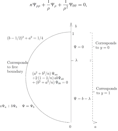
which closes the semicircular domain on which is to be calculated (see Fig. 2). The problem for , comprising (16), (18) and (19), is linear and on a prescribed domain. Note, however, that is determined only up to an arbitrary multiple of a, corresponding to the invariance of (10) to (13) under translations of x.
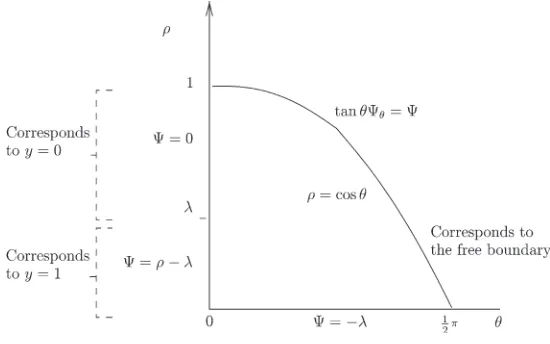
3.1 Polar coordinates
In order to effect an asymptotic solution, it proves helpful to introduce the coordinates(ρ, θ)defined (cf. (13)) by
a = −ρsinθ, b=ρcosθ.
In terms of these, the problem for, comprised of (16), (18) and (19), transforms to
nρρ+1 ρρ+
1
[image:6.536.148.391.334.604.2]ρ2θθ =0, (20)
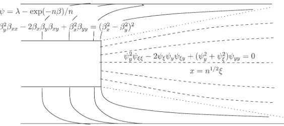
Fig. 3 The formulation in the Legendre plane (polar coordinates)
tanθθ− =0 on ρ=cosθ, (21)
=0 for λ < ρ <1 =ρ−λ for 0< ρ < λ
on θ=0, (22)
= −λ for ρ=0, (23)
where the final condition is added at the singular pointρ = 0 in order to ensure a non-singular solution to the problem; the problem comprised of (20) to (23) determines uniquely up to an arbitrary multiple ofρsinθ. The domain and boundary conditions are shown in Fig. 3
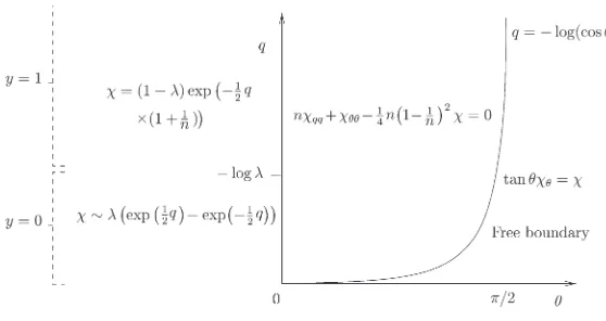
3.2 Logarithmic transform
Before determining an asymptotic solution to this system, we transform the equations a final time by introducing variables
q = −logρ, =λ(e−qcosθ−1)+exp
−1 2
1−1 n
q
χ(q, θ). (24)
Here the first term in (which corresponds to (x,y) = (0, λ), ψ = λ in physical variables) is chosen in order to subtract off the O(1)term in the far-field solution (q → +∞) to reveal important exponentially-small terms inχ. Under the above transformation (20) to (23) is taken to an autonomous PDE (in effect the modified Helmholtz equation), namely
nχqq+χθθ− n 4
1−1 n
2
Fig. 4 The boundary-value problem after the logarithmic transform
with boundary conditions
tanθχθ =χ on q = −log(cosθ), (26) χ=λ
exp q 2
1−1 n −exp −q 2
1+1 n
for 0<q <log
1 λ
χ=(1−λ)exp
−q 2
1+1n
for log 1 λ
<q <∞
⎫ ⎪ ⎪ ⎬ ⎪ ⎪ ⎭
on θ=0,
(27)
χ →0 as q → ∞. (28)
The domain and boundary conditions are illustrated in Fig. 4; the problem comprised of (25) to (28) determinesχuniquely up to an arbitrary multiple of exp(−q(1+1/n)/2))sinθ.
Once the solution forχhas been determined, the positions in physical space of points in the trans-formed plane, and the corresponding streamfunctionψ, can be found from (15); indeed, working backwards through the various transformations gives
x=exp
q 2
1+1
n sinθ
χq−
1 2
1− 1 n
χ
−cosθχθ
, (29)
y=λ−exp
q 2
1+1
n cosθ
χq−
1 2
1−1 n
χ
+sinθχθ
, (30)
ψ=λ−exp
−1 2
1−1 n
q χq+χ
1 2 + 1 2n . (31)
4. Asymptotic solution forψin the Legendre plane 4.1 Region I
of O(1/n)in the form
θ =
n1/2, χ=χ
(I)
0 (q, )+
1 nχ
(I)
1 (q, )+ · · · .
In terms of this new variable, the leading-order problem forχbecomes the quarter-plane formula-tion
∂2χ(I) 0 ∂q2 +
∂2χ(I) 0
∂2 −
χ(I) 0
4 =0, (32)
χ(I)
0 =2λsinh
q
2
for 0<q <log
1 λ
χ(I)
0 =(1−λ)exp
−q 2 for log 1 λ <q ⎫ ⎪ ⎪ ⎬ ⎪ ⎪ ⎭
on =0, (33)
χ(I)
0 →0 as q → ∞, (34)
∂χ( I) 0 ∂ −χ(
I)
0 =0 on q =0, (35)
which here serves a role analogous to that of an inner-diffraction problem in the theory of geomet-rical optics and where the switch in boundary condition on = 0 corresponds to jumping from the centreline of the Hele-Shaw cell (y = 0) to the top boundary (y =1) as q increases through q =log(1/λ). The problem (32) to (35) determines the solutionχ0(I)up to an arbitrary multiple of e−q/2(corresponding to an arbitrary translation in x in the physical plane). Integrating (35) gives
χ(I)
0 =B0 on q =0, (36)
where B0 is an arbitrary constant. Specifying B0 determinesχ0(I) uniquely and hence determines
the x coordinate of the finger tip in the physical plane at O(n1/2)(the subsequent term is required to determine its position up to O(1)). Henceforth we shall take B0 =0 and replace the condition
(35) by
χ(I)
0 |q=0=0. (37)
The problem comprised of (32) to (34) and (37) can be solved by use of a Fourier sine transform χ(I)
0 (q,k)=
∞
0
sin(k)χ0(I)(q, )d, χ0(I)(q, )= 2 π
∞
0
sin(k) χ0(I)(q,k)dk (38) to give
χ(I) 0 =
(1−λ)e−q/2
k +
λ1/2
2k(k2+1/4)1/2
exp
−(k2+1/4)1/2(q−logλ)
−exp
−(k2+1/4)1/2(q+logλ)
, q log(1/λ),
χ(I) 0 =
λ(eq/2−e−q/2)
k +
λ1/2
2k(k2+1/4)1/2
exp
−(k2+1/4)1/2(q−logλ)
−exp
(k2+1/4)1/2(q+logλ)
Here we obtain different forms forχ0(I), depending on whether q>log(1/λ)or q<log(1/λ), as a result of the boundary condition switch in (33). Inversion is best accomplished by writing
χ(I)
0 (q, )=
2 π
∞
0
exp(i k) χ0(I)(q,k)dk
,
and then deforming the contour of integration to make a quarter turn round the pole at k =0 and proceeding up the imaginary axis, so that
χ(I)
0 (q, )=
Res
ei kχ0(I),k=0
+ 2 π
∞
0
e−µχ0(I)(q,iµ)dµ
. (39)
Here (·)and(·)signify the imaginary and real parts of the argument, respectively. We note that the integrand in (39) is purely imaginary forµ ∈ [0,1/2] and that the contribution from the pole at k =0 is zero. It follows that (39) can be rewritten in terms of a real integral (with exponential decay):
χ(I)
0 =
2λ1/2 π
∞
1/2
e−µsin(µ2−1/4)1/2qsin(µ2−1/4)1/2log(1/λ)
µ(µ2−1/4)1/2 dµ. (40)
Leading-order approximations in the physical coordinates can be obtained from (29) to (31) and are, in this region,
x∼ −n1/2exp
q
2
∂χ(I) 0
∂ , y∼λ−exp
q
2
∂χ(I) 0 ∂q −
χ(I) 0
2 + ∂χ(I)
0 ∂
, (41)
ψ∼λ−exp
−q 2
∂χ(I) 0 ∂q +
χ(I) 0
2
. (42)
4.1.2 The finger shape determined by the solution in region I. On the line q=0, corresponding to the finger boundary, we haveχ0(I)=0; thus the expression (42)1for x is zero. A refined
approx-imation of the free-boundary shape, obtained from (29), (30) and expansion of (40), and reflecting the fact that the boundary conditions are actually prescribed on q small but non-zero, is given by
x∼ 1
n1/2
∂χ( I) 0 ∂q −
∂χ(I) 1
∂ −
2
2 ∂2χ(I)
0 ∂∂q
q=0
, (43)
y∼λ−∂χ (I) 0 ∂q
q=0
; (44)
here we use the observation thatχ0(I)|q=0 = 0. The value ofχ1(I)|q=0can be determined (without
solving for χ1(I)) from boundary condition (26), which in terms of the current variables can be written as
n1/2tan
n1/2
∂χ(I)
∂ =χ(I) on q= −log
cos
n1/2
Substitutingχ=χ0(I)+χ1(I)/n+ · · · into the above and expanding up to the O(1)terms gives
∂χ( I) 1 ∂ −χ(
I) 1
q=0 =
1 2
2∂χ( I) 0 ∂q −
3∂χ( I) 0 ∂∂q
−3 3
∂χ(I) 0 ∂
q=0
, (45)
the last term of which is zero sinceχ0(I)|q=0 =0. Differentiating (45) with respect to, dividing
byand integrating with respect togives the following expression for∂χ1(I)/∂|q=0: ∂χ(I)
1 ∂
q=0 =
0 ∂χ(I)
0 ∂q
q=0
d−
2
2 ∂2χ(I)
0 ∂q∂
q=0
+B1, (46)
where B1is an arbitrary constant (corresponding to a translation in x) which we set equal to zero,
thus determining the O(1)term in the expansion of the x-coordinate of the finger tip. Substituting (46) into (43), (44) and using the expression forχ0(I)in (40) gives the following parametrization for the leading edge of the finger:
x ∼ 2λ 1/2 πn1/2
d
d−
, y∼λ−2λ 1/2 π
d
d, (47)
where
(;λ)= −
∞
1/2
e−µsin(µ2−1/4)1/2log(1/λ)
µ2 dµ. (48)
Plots of the finger shape, found by evaluating these formulae numerically, are given in Fig. 7 for various values ofλ.
Large-asymptotic representations of (47) can be found by using Laplace’s method on the inte-gral in (48) to obtain
x∼2λ
1/2log(1/λ) n1/2π1/2
exp(−/2)
1/2 , y∼λ−
2λ1/2log(1/λ) π1/2
exp(−/2)
3/2 as → +∞.
This gives the matching behaviour for the finger shape to be determined, in section 4.3, by the solution in region III. As can be seen from Fig. 6, this corresponds in the physical plane to where the free boundary begins to ‘turn the corner’.
4.1.3 Far-field behaviour ofχ0(I). In order to determine the behaviour ofχ in regions in which θn−1/2and/or q1, it is first necessary to obtain the relevant matching conditions by analysis ofχ0(I)as either or both q→ ∞and→ ∞.
4.1.4 Behaviour ofχ0(I)as → ∞, q = O(1). Applying Laplace’s method to the integral in (40) yields the large-behaviour
χ(I)
0 ∼
2λ1/2log(1/λ)qe−/2
π1/23/2 + · · · as → +∞, q=O(1), (49)
4.1.5 Behaviour ofχ0(I)as→ +∞, q = O(). For the limit in which bothand q simul-taneously tend to∞the process is more involved but can be calculated by deforming the contour of integration into the complex plane and integrating along the path of steepest descent. By making the substitutionµ=s+1/2, the expression (40) can be rewritten as
χ(I)
0 =
2λ1/2
π exp
− 2
∞
0
exp((−s+i h(s+s2)1/2)f(s)ds
, (50)
where
h = q
, f(s)=
sin(s+s2)1/2log(1/λ)
(s+1/2)(s+s2)1/2 . (51)
We now consider the limit→ +∞, h=O(1). The steepest-descent contour is −s+i h(s+s2)1/2= −τ, τ ∈R, τ 0,
and its relevant branch (plotted in Fig. 8(a)) is given by
s= (2τ−h
2)+(h4−4h2(τ+τ2))1/2
2(1+h2) for − ∞< τ <0
(note thatτ =0 corresponds to s=0). For 0< τ < ((1+h2)1/2−1)/2 we have that s∈Rand there is no contribution toχ0(I)from the integral in (50), as the integrand is real. The major contribution toχ0(I)(an end-point contribution) thus comes fromτ just greater thanτ2=((1+h2)1/2−1)/2;
in terms of Fig. 8(a) this is just after the steepest-descent contour leaves the negative real axis at s= −(1−(1+h2)−1/2)/2. This suggests the substitution
τ = (1+h2)1/2−1 2 +t. For small t, we can approximate s in (50) by
s∼ −1 2+
1
2(1+h2)1/2 +i h(1+h
2)−3/4t1/2+ · · ·,
and henceχ0(I)by
χ(I) 0 ∼
2λ1/2 π exp
−(1+h2)1/2 2
× ∞ 0
exp(−t)f
−1 2+
1 2(1+h2)1/2
h(1+h2)−3/4 2t1/2 dt
.
Evaluating the integral and substituting for h from (51) gives, as q→ +∞with=O(q), χ(I)
0 ∼
4λ1/2 π1/2
(2+q2)1/4
sinh
q log(1/λ) 2(2+q2)1/2
exp
−(q2+2)1/2 2
Fig. 5 The asymptotic regions in the Legendre plane (after logarithmic transform) in the limit n→ ∞. In (a) the solid arrows show the transmission of information along the rays of equation (56) from region I to regions IV and V. The dotted arrows represent the rays reflected from the boundary but, because the governing PDE (25) is the modified Helmholtz equation, the contributions of the reflected rays decay exponentially along their paths and are thus of importance only in region IV. In (b) the vertical axis has been compressed in order to show region VII
Fig. 6 A sketch of the asymptotic regions in the physical plane in the limit n→ ∞; compare with Fig. 5
wherein the preexponential factor corresponds (in analogy with canonical diffraction problems) to the directivity associated with the expansion fan emanating from this region (cf. Fig. 5(a)).
[image:13.536.138.398.392.514.2]Fig. 7 The leading-order finger shape (in the physical plane), which is independent of n in the coordinates shown, determined by the solution in region I; this corresponds to the leading edge of the finger. Here we have, moving up the y-axis,λ=0·1,0·2, . . . ,0·9. The x origin has been fixed by the choices B0=B1=0, leading
here to the intersection of the finger with the x-axis varying non-monotonically withλ
different asymptotic behaviour arising where q → +∞with = O(q1/2). Here we again make the substitutionµ=s+1/2 in (40) and rewriteχ0(I)in the form
χ(I)
0 =
2λ1/2 π
∞
0
exp(i q(s+s2)1/2)g(s)ds
,
where
g(s)=exp
−
s+1 2
sin(s+s2)1/2log(1/λ) (s+1/2)(s+s2)1/2 .
The steepest-descent contour is now given by i q(s+s2)1/2= −τ, whereτ is real and positive and is plotted in Fig. 8(b). It follows that
s=−1+(1−4τ
2/q2)1/2
2
Fig. 8 The steepest-descent contours used for calculating the asymptotic behaviour ofχ0(I). The dashed line is a branch cut running between the branch points at s=0 and s= −1
χ(I) 0 =
2λ1/2 π
πi 2 Res
exp(i q(s+s2)1/2)g(s),s= −1/2
+
−1/2+i∞
−1/2
exp(i q(s+s2)1/2)g(s)ds
.
Evaluating the residue and making the substitution s= −1/2+i(t+t2)1/2gives χ(I)
0 =
2λ1/2e−q/2 π
πsinh
log(1/λ) 2
−
∞
0
sin((t+t2)1/2)sinh((t+t2)1/2log(1/λ))
(t+t2) e
−qtdt
.
The integral in the above expression may be approximated in the limit q→ +∞,=O(q1/2)by writing=q1/2γ, making the substitution t=τ/q and expanding in powers of q; this gives
∞
0
sin(γq1/2(t+t2)1/2)sinh((t+t2)1/2log(1/λ))
(t+t2) e
−qtdt
∼sinh
log(1/λ) 2
∞
0
sin(γ τ1/2)
τ e−τdτ =πsinh
log(1/λ) 2
erf
γ
2
,
where erf(·)is the error function. It follows that the asymptotic behaviour ofχ0(I)is χ(I)
0 ∼(1−λ)e− q/2
1−erf
2q1/2
as q→ ∞ with
Note that this expression satisfies the boundary conditionχ0(I) = (1−λ)e−q/2 on = 0 and matches to the behaviour (52) as /q1/2 → ∞. The leading-order solution (53) is of ‘shadow-boundary’ type, corresponding to the parabolic approximation to the modified Helmholtz equation. The presence of the various sublayers we have described in the far field ofχ0(I) is reflected in the full asymptotic structure of the solutions in the limit n→ ∞(cf. Fig. 5). We now proceed to discuss region II, into which the expansion fan solution (52) matches.
4.2 Region II
We look for a solution forχ = χ(II)(q˜, θ), in a region in which q = O(n1/2)andθ = O(1), by introducing the new coordinate q=n1/2q. With this rescaling, equation (25) becomes˜
∂2χ(II) ∂q˜2 +
∂2χ(II) ∂θ2 −
n 4
1−1 n
2
χ(II)=0. (54)
An asymptotic solution to this can be found by using a WKBJ ansatz χ(II)= 4λ1/2n−1/4
π1/2 exp
n1/2h0(q˜, θ) H0(˜q, θ)+
1
n1/2H1(q˜, θ)+ · · ·
. (55)
To leading order this gives an Eikonal equation for h0, h20,θ+h20,q˜ =1
4. (56)
Solving subject to initial conditions obtained by matching to (52) asq˜ → 0 andθ → 0 gives the expansion fan solution
h0= −
˜
q2+θ21/2
2 .
Proceeding to next order in the expansion yields the amplitude equation 2θH0,θ+ ˜q H0,q˜
+H0=0
for H0, with general solution
H0=θ−1/2P
˜
q θ
,
where the ‘directivity’ P(·)is a function which is determined by matching with (52) asq˜ →0 and θ→0, so that
H0(q˜, θ)=
4λ1/2n−1/4 π1/2
(θ2+ ˜q2)1/4
θ sinh
1 2
˜
q log(1/λ) (q˜2+θ2)1/2
, (57)
from which we deduce that the WKBJ ansatz (55) gives the following asymptotic formula forχ(II) as n→ ∞:
χ(II)∼4λ1/2n−1/4 π1/2
(θ2+ ˜q2)1/4
θ sinh
1 2
˜
q log(1/λ) (q˜2+θ2)1/2
+O
n−1/2
×exp
−n1/2(q˜
2+θ2)1/2
2
Note that this solution does not satisfy the boundary condition (26) onθ ∼ π/2−exp(−n1/2q˜) (that is, on q = log(cosθ)) and it will therefore be necessary to introduce a further region in the vicinity of the boundary (namely region IV).
Physical coordinates may be found by substituting the solution ansatz (55) into (29) to (31); this gives
x∼ 2λ 1/2n1/4 π1/2 exp
−n1/2 2 ((q˜
2+θ2)1/2− ˜q)
θ
(q˜2+θ2)1/2cosθH0(q˜, θ),
y∼λ+2λ 1/2n1/4 π1/2 exp
−n1/2 2 ((q˜
2+θ2)1/2− ˜q)
θ
(˜q2+θ2)1/2sinθH0(q˜, θ),
ψ∼λ−2λ1/2n−1/4 π1/2 exp
−n1/2 2 ((q˜
2+θ2)1/2+ ˜q) 1− q˜ (q˜2+θ2)1/2
H0(q˜, θ),
(59)
where H0is given by (57). Rewriting these in terms of the radial coordinates r =(x2+(y−λ)2)1/2
andφ=arctan((y−λ)/x)gives
r ∼2λ 1/2n1/4 π1/2 exp
−n1/2 2 ((q˜
2+θ2)1/2− ˜q)
θ
(q˜2+θ2)1/2H0(q˜, θ), φ∼θ,
log(λ−ψ)∼ − nφ
2
4 log(1/r).
(60)
4.3 Region III
4.3.1 Leading-order solution. We now look for an asymptotic solution to (25), (26) in the region in which both q andθare O(1)by making the WKBJ ansatz
χ(III)(q, θ)∼2λ1/2log(1/λ)n−3/4 π1/2 exp
−n1/2θ
2 G0(q, θ)+n −1/2G
1(q, θ)+ · · ·
. (61)
Here the dominant behaviour log(χ(III))∼ −n1/2θ/2 is a consequence of matchingχ(III), in the limit q→ ∞, toχ(II). To next order this ansatz gives
G0,qq =0⇒G0=A(θ)q+B(θ),
the reason for this trivial balance being that the region is essentially a passive one, required simply to moderate the ray solution in order to fit the boundary conditions (the boundary is perturbed from q =0 by an amount that is asymptotically much smaller than the q scaling corresponding to the parabolic approximation). HereA(·)and B(·)are functions that are determined by matching to region II in the limit q → ∞and applying the boundary condition (26) on q = −log(cos(θ)) (which givesA(θ)q+B(θ)|q=−log(cos(θ))=0), so that
G0(q, θ)=
q+log(cosθ)
Substitution of G0back into (61) implies that χ(III)∼ 2λ1/2log(1/λ)n−3/4
π1/2
q+log(cosθ) θ3/2 +n
−1/2G
1(q, θ)+ · · ·
exp
−n1/2θ 2
. (63)
The correction term n−1/2G1(q, θ) is included here because it appears in the calculation of the
finger shape and needs (for this purpose) to be evaluated on q = −log(cosθ), but not elsewhere. Proceeding to first order in the expansion of (26) gives
tanθ
G0,θ− G1
2
=G0 on q= −log(cosθ),
from which it follows that
G1|q=−log(cos(θ))= −
2 tanθ
θ3/2 . (64)
The physical quantities may be found by substituting the solution ansatz (61) into (29) to (31); this gives
x∼ λ
1/2log(1/λ)n−1/4 π1/2 exp
−n1/2 2 θ
G0eq/2cosθ,
y∼λ+λ
1/2log(1/λ)n−1/4 π1/2 exp
−n1/2 2 θ
G0eq/2sinθ,
ψ∼λ−2λ1/2log(1/λ)n−3/4 π1/2 exp
−n1/2 2 θ
e−q/2
G0,q+ G0
2
,
(65)
where G0is given by equation (62). Again rewriting these in terms of the radial coordinates r = (x2+(y−λ)2)1/2andφ=arctan((y−λ)/x)gives
r∼ λ
1/2log(1/λ)n−1/4 π1/2 exp
−n1/2 2 θ
G0eq/2, φ∼θ,
log(λ−ψ)∼ −n
1/2
2 φ.
(66)
4.3.2 Finger shape determined by the solution in region III. The leading edge of the finger (as determined by the solution in region I) is almost flat, lying approximately parallel to the y-axis. The shape of the finger as it rounds the ‘corner’, away from the vertical, is determined by expanding the solution in region III in powers of n along q= −log(cos(θ)), and substitution into equations (29), (30). To the relevant orders this gives the following expressions for x(θ)and y(θ):
x∼ 2λ
1/2log(1/λ)n−3/4 π1/2 exp
−n1/2θ 2
(cosθ)−1/2
2sinθ θ3/2 +
cosθ
2 G1(q, θ)
q=−log(cos(θ)) ,
y∼λ−2λ
1/2log(1/λ)n−3/4 π1/2 ×exp
−n1/2θ 2
(cosθ)−1/2
secθ θ3/2 +
sinθ
2 G1(q, θ)
Substituting for G1|q=−log(cosθ), using (64), gives the finger shape parametrized byθ
x∼2λ
1/2log(1/λ)n−3/4 π1/2
sinθ
θ3/2(cosθ)1/2exp
−n1/2θ 2
, (67)
y∼λ−2λ
1/2log(1/λ)n−3/4 π1/2
(cosθ)1/2 θ3/2 exp
−n1/2θ 2
. (68)
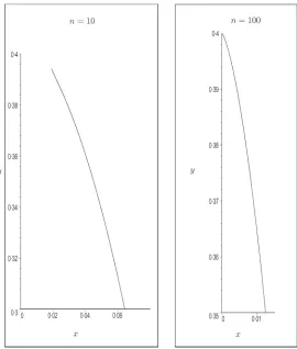
[image:19.536.134.404.209.527.2]The finger shape is plotted, forλ=0·4 and n=10 and n=100, in Fig. 9.
4.4 Region IV
As already noted, the asymptotic solution for χ in region II (namelyχ(II)) does not satisfy the boundary condition (26). In region IV, shown schematically in Fig. 5, this manifests itself in a different way from in region III and thus needs separate discussion. Thus we introduce a further region in the vicinity of the boundary q= −log(cosθ)defined by the variables
θ= π 2 +
ν
n1/2, q =n
1/2q˜, χ=χ(IV)(q˜, ν).
In terms of these new variables the boundary is approximated byν∼ −n1/2exp(−n1/2q˜)andχ(IV) satisfies
∂2χ(IV) ∂ν2 −
1 4
1−1 n
2
χ(IV)+ 1 n
∂2χ(IV)
∂q˜2 =0 forν <−n
1/2exp(−n1/2q˜)+ · · · , (69)
χ(IV)+n1/2cot ν n1/2
∂χ(IV)
∂ν =0 onν= −n1/2exp(−n1/2q˜)+ · · ·. (70) An approximate solution to this system can be obtained by making the WKBJ ansatz
χ(IV)= 16λ1/2n−1/4 π3/2
W0(q˜, ν)+n−1/2W1(q˜, ν)+ · · ·
exp(−n1/2w0(q˜)). (71)
Matching to region II in the limit ν → −∞ gives w0(˜q) = −12(q˜2 +π2/4)1/2. Substituting χ(IV)into (69), (70) and taking the leading-order term gives the following equation and boundary
condition for W0:
W0,νν−
1 16
π2 (q˜2+π2/4)1/2
W0=0, and W0,ν|ν=0=0,
with solution
W0=D(q˜)cosh
πν
4(π2/4+ ˜q2)1/2
. (72)
HereD(·)is a directivity which is determined by matching to the solution in region II in the limit ν → −∞. Proceeding with the matching (in order to determine D) and substituting the result, together with the expression forw0(q˜), back into the ansatz forχ(IV)gives the following asymptotic
formula forχ(IV)as n→ ∞: χ(IV)∼16λ1/2n−1/4
π3/2 exp
−n1/2(q˜
2+π2/4)1/2
2
(q˜2+π2/4)1/4
×sinh
1 2
˜
q log(1/λ) (˜q2+π2/4)1/2
cosh
πν 4(q˜2+π2/4)1/2
. (73)
Again physical coordinates may be found by substituting the solution ansatz (61) into (29) to (31). In this case we find
x∼ 16λ 1/2 π3/2 n−
1/4exp
⎛ ⎝−n1/2
2
⎛ ⎝
˜ q2+π
2
4
1/2 − ˜q
⎞ ⎠ ⎞ ⎠ ×
νW0,ν−
1 2
1+ q˜ (q˜2+π2/4)1/2
W0
,
y∼λ−16λ 1/2 π3/2 n
1/4exp
⎛ ⎝−n1/2
2
⎛ ⎝
˜ q2+π
2
4
1/2 − ˜q
⎞ ⎠
⎞ ⎠W0,ν,
ψ∼λ−8πλ31//22n−1/4exp
⎛ ⎝−n1/2
2
⎛ ⎝
˜ q2+π
2
4
1/2 + ˜q
⎞ ⎠
⎞
⎠1− q˜ (q˜2+π2/4)1/2
W0,
(74)
where W0is given by (72).
4.5 Region V (the corner region)
This corresponds to a second inner diffraction problem and gives the most difficult leading-order balance. However, because the rays that emerge from this region carry exponentially small contri-butions to the solution elsewhere, this need not trouble us unduly (though see section 6 for some pertinent remarks). Here we introduce the scaled variables
θ =π 2 +
ν
n1/2, q =
1
2log n+s, χ =χ
(V)(s, ν), (75)
in terms of which equation (25) and boundary condition (26) can be rewritten as n
∂2χ(V) ∂s2 +
∂2χ(V) ∂ν2 −
χ(V)
4
+χ(V) 2 −
χ(V)
4n =0, (76)
χ(V)+n1/2cot ν n1/2
∂χ(V)
∂ν =0 on ν = −e−
s. (77)
Matching to regions II, III and IV respectively gives far-field conditions onχ(V): χ(V)∼P(n, λ)e−ν/2
1
2log n+s
as ν→ −∞ s→ +∞ (s=O(ν)), (78) χ(V)∼P(n, λ)e−ν/2(log(−ν)+s) as ν → −∞ s→ −∞ (s=O(log(−ν))), (79) χ(V)∼P(n, λ)
2 cosh
ν
2 1
2log n+s
as s→ +∞ (ν=O(1)), (80) wherePis an exponentially small quantity defined by
P(n, λ)=
4√2λ1/2log(1/λ) π2
n−3/4exp
−n1/2π 4
The expansion forχ(V)thus proceeds in the form χ(V)≡P(n, λ)log nχ(V)
0 +χ
(V) 1 + · · ·
. (82)
The first two terms satisfy ∂2χ(V)
0 ∂s2 +
∂2χ(V) 0 ∂ν2 −
χ(V) 0
4 =0,
∂χ(V) 0 ∂ν
ν=−e−s
=0, (83)
χ(V)
0 →0 asν→ −∞, s→ −∞ (s=O(log(−ν))), χ(V)
0 ∼
e−ν/2
2 asν→ −∞, s→ +∞ (s=O(ν)), χ(V)
0 ∼cosh
ν
2
as s→ ∞ (ν=O(1)); ∂2χ(V)
1 ∂s2 +
∂2χ(V) 1 ∂ν2 −
χ(V) 1
4 =0,
∂χ(V) 1 ∂ν
ν=−e−s =0,
χ(V)
1 ∼e−ν/2(log(−ν)+s) asν→ −∞, s→ −∞ (s=O(log(−ν))), χ(V)
1 ∼se−ν/
2 asν→ −∞, s→ +∞ (s=O(ν)), χ(V)
1 ∼2s cosh
ν
2
as s→ +∞ (ν=O(1)). (84) These two problems require the solution of a linear elliptic PDE on a non-separable domain; they are unlikely to be amenable to standard analytical techniques. Note, however, that the problems for χ(V)
0 andχ( V)
1 are canonical—that is, they do not depend upon eitherλor n.
The physical quantities in this regime are found by substituting the solution ansatz (75) and (82) into (29) to (31), to give
x∼P(n, λ)n1/4log nes/2
∂χ(V) 0 ∂s −
χ(V) 0
2 +ν ∂χ(V)
0 ∂ν
,
y∼λ−P(n, λ)n3/4log nes/2∂χ (V) 0 ∂ν ,
ψ∼λ−P(n, λ)n−1/4log ne−s/2
∂χ(V) 0 ∂s +
χ(V) 0
2
,
(85)
4.6 Region VI
The differing asymptotic behaviours of χ0(I) as q → +∞ with (i) = O(q) (see (52)), and (ii) with=O(q1/2)(see (53)) suggest thatχ0(I)matches, as q → +∞, to different asymp-totic regions in which either (i) n1/2θ = O(q), as in region II, or (ii) n1/2θ = O(q1/2). Here we treat the latter case, the former being treated in section 4.2, by introducing the scaled coordinates
q=n1/2q˜, θ =n−1/4θ,˜
in terms of which the governing equation (25) and boundary condition (27)2are ∂2χ(VI)
∂q˜2 +n
1/2∂2χ(VI) ∂θ˜2 −
n 4
1−1 n
2
χ(VI)=0, (86)
χ(VI)|
θ=0∼(1−λ)exp
−n1/2q˜ 2
1+1 n
. (87)
Asθ˜ → +∞and asq˜ → 0 two further conditions can be obtained by matching to region II and region I (via (53)); these are, respectively
χ(VI)∼ 2
π1/2(1−λ) ˜ q1/2
˜ θ exp
−θ˜2 4q˜
exp
−n1/2q˜ 2
as θ˜→ ∞,
χ(VI)∼(1−λ)exp
−n1/2q˜
2 1−erf
˜ θ 2q˜1/2
as q˜→0 with θ˜=O(q˜1/2).
Making the WKBJ ansatz
χ(VI)=
f0(q˜,θ)˜ +
1
n1/2f1(q˜,θ)˜ + · · ·
exp
−n1/2q˜ 2
and substituting into (86) to (88) leads to the following initial-value problem for f0(corresponding
to the parabolic approximation in diffraction theory): f0,q˜= f0,θ˜θ˜,
f0|q˜=0=0, f0|θ˜=0=(1−λ), f0→0 asθ˜→ ∞,
with solution
f0=(1−λ)
1−erf
˜ θ 2q˜1/2
(cf. a shadow boundary in diffraction theory) so that
χ(VI)∼(1−λ)exp
−n1/2q˜
2 1−erf
˜ θ 2q˜1/2
Physical quantities may be found by substituting the solution ansatz (61) into (29) to (31). In this case we find
x= −n1/4f0,θ˜+O(n−1/4), y=λ+(f0− ˜θf0,θ˜)+O(n−1/2), (89) ψ∼λ−n−1/2exp(−n1/2q˜)(f0,q˜+O(n−1/2)), (90)
and approximate streamlines have constantq and are shown in Fig. 10. Substituting for f˜ 0in the
above we obtain x
n1/4 = (1−λ)
π1/2
exp(−η2) ˜
q1/2 +O(n−
1/2), y=1+(1−λ)
2
π1/2ηexp(−η
2)−erf(η)
,
log
n1/2(λ−ψ)
= −n1/2q˜+O(1),
whereη = ˜θ/(2q˜). It is apparent that, to leading order, y is a function of ηonly. Hence, if we introduce a function H defined by
H(y0(η))= (
1−λ)2
π exp(−2η2), y0=1+(1−λ)
2
π1/2ηexp(−η
2)−erf(η)
,
where y0(η)is the leading term in the expansion of y, we obtain
log(n1/2(λ−ψ))∼ −n1/2H(y)
ξ2 , (91)
whereξ = x/n(1/4). Note that y0 → λ+as η → +∞and that y0 = 1 atη = 0. Furthermore,
although H does not tend to infinity as y→1−its derivative d H/d y does. The fact that H remains finite on y=1 despite the exact boundary condition beingψ|y=1=0 is indicative of the existence
of an additional boundary layer (about y=1) in the physical plane. 4.7 Region VII
Finally, we consider an extension of region VI, that is influenced directly by the finger boundary q = −log(cosθ), and the channel wallθ=0 by introducing the scaled coordinate
q =n Q.
In terms of Q the governing equation (25) and boundary conditions (27), (28) are 1
n
∂2χ(VII) ∂Q2 +
∂2χ(VII) ∂θ2 −
n 4
1−1 n
2
χ(VII)=0, (92)
χ(VII)|
θ=0=(1−λ)exp
−nQ 2 −
Q 2
, (93)
tanθ∂χ (VII)
∂θ −χ(VII)=0 on θ =arccos(e−n Q). (94) Matching to region II as Q→0 leads to the further condition
χ(VII) ∼
2(1−λ) π1/2
Q1/2 θ exp
−θ2 4Q
exp
−n Q 2
in view of which we make the WKBJ ansatz χ(VII) =
g0(Q, θ)+
1
ng1(Q, θ)+ · · ·
exp
−n Q 2
,
leading to the following initial-value problem for g0(which is again a parabolic approximation): g0,Q =g0,θθ +
g0
2, (95)
g0|θ=0=(1−λ)exp
−Q 2
, g0,θθ=π/2=0, (96)
g0|Q=0=0, g0→0 as Q→ ∞. (97)
We also require the inversion formula, (29) to (31), to give the variables x,y, ψ, these being ap-proximated by
x∼ −exp
Q
2 g0sinθ+g0,θcosθ
, y∼λ−exp
Q
2 g0,θsinθ−g0cosθ
,
ψ∼λ−n−1exp
−n Q+ Q
2 g0,Q+ g0
2
.
(98)
Solving (95) to (97) for g0gives
χ(VII)∼g
0(Q, θ)exp
−nQ 2
,
g0=
2(1−λ)
π exp(−Q/2)
2Q sinθ+
π
2 −θ
cosθ
+∞ m=0
Amsin((2m+1)θ)exp
−
(2m+1)2−1 2
Q
,
A0= −
1−λ
π , Am = −(
1−λ) π
1 m+1 +
1 m
for m1.
The finger boundary (corresponding toθ∼π/2) decays exponentially as x → −∞to the constant value y =λ. To leading order, the streamlines are given by the level sets of Q except (in view of (98)3) close to the lineθ=0, on which g0,Q+g0/2=0. These streamlines are plotted in Fig. 10.
5. The physical plane
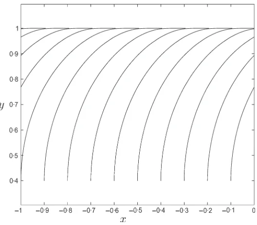
Fig. 10 Approximate streamlines in the physical plane determined from regions VI and VII of the Legendre plane. From the bottom right the streamlines in VII areq˜ = 0·02,0·05,0·1,0·2,0·5,1,2,5 (where q˜ ∼
−log(n1/2(λ−ψ))/n1/2), while in (VII) they are Q =0·05,0·1,0·2, . . . ,0·9,1·0 (where Q ∼ −log(λ− ψ)/n). The finger corresponds under these scalings to the semi-infinite strip x <0 (that is,ξ <0),−0·4< y<0·4. Asq˜ → +∞in region VI the solution matches into the solution in region VII as Q→0
Fig. 11 A schematic of the streamlines in the physical plane, together with the leading-order equations. In the regions where the streamlines correspond to rays they are shown as solid lines. Divisions between regions are shown in dotted lines
5.1 Remarks on the merits of solving in the Legendre plane versus those of solving in the physical plane
[image:26.536.128.410.319.444.2]5.2 Slowly varying region in front of the advancing finger (region I)
In light of the scalings derived in section 4.1.2, that is (42), we rewrite (10) to (13) by rescaling x according to
x =n1/2ξ and writing the free boundary in the form
ξ = 1
n(y;n);
since=O(1), this will allow us to linearize the free-boundary conditions ontoξ =0 (we remark that the scalings x= O(1)and x = O(n−1/2)might also be thought pertinent in approaching the free boundary, but these regions turn out to be entirely passive,ψbeing given by the inner limit of theξ =O(1)solution). Thus (10) to (13) give
ψ2 y +
1 n2ψ
2
ξ
ψξξ−2
1−1 n
ψξψyψξy+(ψy2+ψξ2)ψyy=0, (99)
−(y)ψy+ψξξ=(y)/n,0<y<λ=0, ψ|ξ=(y)/n,0<y<λ=y, (100) ψ|y=0=0, ψ|y=1=λ, ψ→λy asξ → ∞. (101)
Expandingψandin powers of 1/n in the form ψ=ψ(I)
0 +
1 nψ
(I)
1 + · · · , =0+ · · · ,
and substituting into (99) to (101) leads to an elliptic boundary-value problem forψ0(I), namely ψ(I)
0 2
yψ
(I)
0 ξξ−2ψ( I) 0 ξψ(
I) 0 yψ(
I) 0 ξy+
ψ(I) 0
2
y+ψ
(I) 0
2
ξ
ψ(I)
0 yy=0, (102) ψ(I)
0 |ξ=0,0<y<λ=y, ψ0(I)|ξ=0,λ<y<1=λ, (103) ψ(I)
0 |y=0=0, ψ( I)
0 |y=1=λ, ψ( I)
0 →λy asξ → ∞. (104)
Here (102) is the inverse Legendre transform of (32) and the condition (103)2arises from matching
into region VI whereλ−ψis exponentially small. Finally (100)1gives rise to a condition which
determines the shape of the free boundary
0(y)= ψ(I)
0 ξ ψ(I)
0 y
ξ=
0,y<λ .
Noteworthy features of the solution in this region are (i) that the finger shape, determined here, is to leading order flat running parallel to the y-axis between y= −λand y=λ, and (ii) that the Aron-sson ray approach does not apply in this outer region (slowly varying in x) despite a significant fluid flow. We remark also that (102) has an interesting status as a limit problem of (1)1, notably in that it
formulation remains elliptic—this may be contrasted with linear elliptic problems whose standard slender approximations are parabolic; we observe that in divergence form it reads (on dropping the suffices) as ∂ ∂ξ ψ ξ ψy +∂∂ y
logψy−
1 2 ψ2 ξ ψ2 y
=0.
5.3 Reformulation in polar coordinates
At this stage it is useful to introduce polar coordinates about the finger ‘corner’ (we now choose the origin of x to fix this at(x,y)=(0, λ)by setting B0=B1=0 in (36) and (46))
r=
x2+(y−λ)2
1/2
, φ=arctan
y−λ x
, (105)
in terms of which (10) and (11) can be written as
ψ2
φ r2 +
ψ2 r n
ψrr−2
1−1 n
ψrψφψrφ r2 + 1 r2 ψ2 r + ψ2 φ nr2
ψφφ+ψ
3 r
r +
2−1 n
ψ
rψφ2
r3 =0, (106)
ψrNr +ψφ r Nφ
∂f
=0, ψ|∂
f =λ+r sinφ, (107)
where the normal to the boundary is N=Nrer+Nφeφ.
The physical domains corresponding to all of the regions II, III and IV of the Legendre plane lie close to(x,y)=(0, λ). In order to determine the solution in these regions it is convenient to use the formulation (106), (107). In addition, we need to introduce a stretched variable R, to describe the free boundary in terms of R via
r=exp(−n1/2R), R|∂=F(φ) and to rewriteψin the WKBJ form
ψ=λ−exp(−n1/2ϒ(R, φ));
thus r is exponentially close to zero andψtoλ. In terms of these new variables (106), (107) give ϒ2
φ
ϒR+ϒφ2
+1 n
ϒ3
R+2ϒR2ϒφ2−ϒRϒφ2
+ 1 n2
ϒ4 R−ϒR3
= 1 n1/2
ϒR Rϒφ2−2ϒRϒφϒRφ+ϒφφ
ϒ2 R+ϒφ2
+ 2
n3/2ϒRϒφϒRφ+
1 n5/2ϒ
2
RϒR R, (108)
n F(φ)∂ϒ ∂φ −
∂ϒ ∂R
R=F(φ)
=0, ϒ|R=F(φ)=F(φ)−
1
In addition we must impose the far-field condition
ϒ→ +∞ as R→0+ withφ >0, (110)
which is equivalent to requiring thatψ∼λfor r=O(1)andφ >0.
5.4 Regions II and III
The expansion forϒin regions II and III proceeds as follows: ϒ =ϒ0+
log n n1/2ϒ1+
1
n1/2ϒ2+ · · ·,
and gives, on substitution into (108),
∂ϒ0 ∂φ
2∂ϒ 0 ∂R +
∂ϒ0 ∂φ
2 =0.
This factorization corresponds to two distinct regions, II and III.
5.4.1 Region II. Here the leading-order balance is ∂ϒ(II)
0 ∂R +
∂ϒ(II) 0 ∂φ
2 =0,
corresponding to equation (56) in the Legendre plane. Imposing the far-field condition (110) speci-fies the solution uniquely as
ϒ(II)
0 =
φ2
4R. In turn this implies that
log(λ−ψ(II))∼ −n φ 2
4 log(1/r).
5.4.2 Region III. Here the solution satisfies the following leading-order balance and boundary condition (derived from (109)):
∂ϒ(III) 0
∂φ =0,
∂ϒ(III) 0 ∂φ
R=F(φ)
=0, ϒ0(III)
R=F(φ)=F(φ),
and consequently has solution ϒ(III)
5.5 Region IV
In light of the scalings derived from region IV of the Legendre plane (74) we look for a solution in region IV of the physical plane of the form
ϒ(IV)=ϒ(IV)(R,φ),¯ where φ= π
2 + ¯ φ n1/2.
Going to leading order givesϒ(IV)
0,φ¯ = 0 so, in light of (74) we expect ϒ
(IV)
0 (R) = π2/(16R);
however, this requires some tricky matching to region II to confirm this. 5.6 Region V
In light of the scalings (85) in the Legendre plane, we look for a solution in region V of the physical plane of the form
x=n−1/2log n exp
−n1/2π 4
X, y=λ−log n exp
−n1/2π 4
Y,
ψ(V)=λ−n−1log n exp
−n1/2π 4
ˆ ψ,
and a free boundary shape described by
Y = 1 n(X).
Substituting the above into (10) to (13) gives the following problem forψˆ:
ˆ ψ2
Y + ˆψ2X
ˆ ψX X−2
1− 1 n
ˆ
ψXψˆYψˆX Y +
ˆ ψ2
X+
1 n2ψˆ
2 Y
ˆ
ψY Y =0, (111)
−(X)ψˆX+ ˆψY
Y=(X)/n=0, ψˆ
Y=(X)/n =(X). (112)
The expansion ofψˆ in region V proceeds as follows: ˆ
ψ= ˆψ0+
1
log nψˆ1+ · · · ,
and the equation satisfied byψˆ0corresponds to (83) in the Legendre plane, (111) being equivalent
to (102) but with the roles of x and y interchanged, and the free-boundary conditions similarly linearize on to Y=0, where
ˆ
ψ0,Y = ˆψ02,X.
5.7 The problem about the top edge of the finger (region VII)
In light of the scalings for the physical variables (98) derived in section 4.7 we look for a solution in the physical plane, along the top edge of the finger (see Fig. 6), of the form
ψ=λ−1
Substituting this ansatz into (6) gives
β2 y+
1 nβ
2 x
βx x−2
1−1 n
βxβyβx y+
β2 x+
1 nβ
2 y
βyy=
β2 x+β2y
2
. (114) On the upper boundary (13)1gives
β→ +∞ as y1. (115)
The conditionψ|∂=y implies that the finger shape is given by y=λ−1
n exp(−nβ), while (11)1gives
βy− |∇β|2e−nβ
y=λ−exp(−nβ)/n=0.
Linearizing on to y=λgives the approximate boundary condition
βy|y=λ=0. (116)
To close the problem forβ we match to the main flow (corresponding to region I of the Legendre plane); this gives
β ∼O
1 n
as x→ +∞, β∼O
1 n
as y→λ with x >0. (117) Whilst it is not possible to solve the full problem comprised of (114) to (117), without recourse to Legendre or Hodograph transforms, we can solve this problem in the limit x → −∞. This subproblem is invariant under translations of x andβ, which suggests looking for a solution of the form
β0= −kx+G(y).
This gives rise to the following problem for G and k:
k2+1 n
d G d y
2d2G
d y2 =
k2+
d G d y
22
, (118)
d G d y
y=λ
=0, (119)
G→ ∞ as y→1, (120)
which, on introduction of the variable z =d G/d y, can be analysed by use of a phase plane. The naive asymptotic expansion G=G0+O(1/n)gives rise to a leading-order equation for G0which
is incompatible with the boundary condition (120). In order to overcome this difficulty we introduce an outer region in which 1−y=O(1), and on which the boundary condition
d G/d y→ ∞ as y→1 (121)