Contents
Executive summary 6
1 Introduction 8
2 Who benefits most from globalization? 9
2.1 Methodology 10
2.1.1 Determining the “globalization champion” 10 2.1.2 Scenarios for future globalization developments 16
2.2 Globalization index: results 19
2.2.1 Descriptive analysis of the globalization index 19 2.2.2 Regression analyses on the correlation between globalization
and economic growth 26
2.3 Growth effects of globalization 29
2.3.1 Determining the globalization champion based on income gains per capita 31 2.3.2 Globalization-induced income gains per capita in relation to the starting level 35 2.3.3 Globalization-induced income gains at the country level 37 2.3.4 Overall globalization gains in comparison to the gross domestic product 39 2.3.5 Income gains per capita in relation to changes in income distribution 39 2.4 Future scenarios for globalization developments 44 2.4.1 “Accelerated globalization” results scenario 44 2.4.2 “Diverging globalization” results scenario 49
3 The most appealing foreign markets 57
3.1 Focus and methodology of the Prognos Free Trade and Investment Index 58
3.2 The most appealing foreign markets 2013 60
4 Bibliography 67
5 Appendix A – Additional tables 68
6 Appendix B – Additional figures 75
Executive summary
The “Globalization report 2014: Who benefits most from globalization?” study comprises two parts. The first part focuses on the question to what extent different countries have benefited from globalization in the past and to which degree this is possible in the future. The second part uses the Prognos Free Trade and Investment Index to offer a differentiated measure for the attractiveness of foreign markets for German companies.
The methodology of the ex-post analysis in the first section of the report is based on scenario calculations for 42 countries during the period 1990–2011. One scenario assumes that globalization has not progressed further since the beginning of the study period. The comparison of this scenario and the actually observed economic development then allows the quantification of globalization-induced gains in added value and a comparison across nations.
Key findings of the ex-post analysis based on scenario calculations can be summarized as follows:
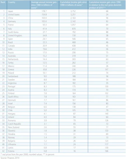
• If we add up the differences in the gross domestic product per capita between the scenario and the historically observed development over the entire study period, Finland achieves the greatest globalization gains among all the countries under review, with an annual average of €1500 per capita. From this perspective, Germany ranks in the top third along with many
smaller European countries. By contrast, the large developing nations finished exclusively at the bottom of the ranking.
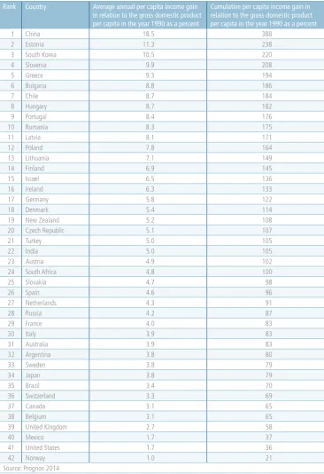
• The weak positions of developing nations – especially that of China – can be traced back among other things to the low economic output per capita in the initial year of the study period. As such, the average annual globalization-induced income gain per capita in relation to the gross domestic product per capita in 1990 was around 18.5 percent for China, compared to just under 6 percent for Germany and a mere 2 percent for the United States.
The essential results of the projections can be summarized as follows:
• The “accelerated globalization” scenario shows that Eastern European countries and major developing nations in particular can anticipate elevated growth rates of around 0.5 percentage points until the year 2020, if the pace of globalization were to increase by 50 percent. By contrast, significantly lower growth could be anticipated for major national economies with a high per capita income.
• In the “diverging globalization” scenario, declines in growth are, as anticipated, most extreme in the countries that are directly affected by the modeled stagnation in globalization: Greece, Portugal and Spain. By the year 2020, these nations would lose up to one percentage point in yearly economic growth. National economies that would indirectly suffer the heaviest impact, such as Italy, are key trade partners of the directly affected countries.
The Prognos Free Trade and Investment Index – the main component of the study’s second part – bundles a broad spectrum of economic, institutional and sociopolitical indicators into a comprehensive measure of the attractiveness of foreign markets for German companies. While the presentation as a ranking ensures clarity, the large number of countries under consideration and a high degree of detail in the set of indicators enable us to recognize the foreign markets whose appeal for German companies is still underestimated so far.
The key findings of the analysis based on the Prognos Free Trade and Investment Index can be summarized as follows:
• The Prognos Free Trade and Investment Index shows that despite the current crisis in the European Union and especially in the euro zone countries, the most attractive conditions for foreign activities by German decision makers continue to be found in European nations.
1 Introduction
The increasing economic, political and social interconnectedness of the world is ubiquitous. It is evident in the steadily rising sales of German mechanical construction companies beyond the country’s borders as well as in the fact that more Asians use Facebook than North Americans and that the United Nations now has almost as many members as there are sovereign states. As different as they may seem, all of these developments are manifestations of a worldwide phenomenon – globalization.
No one disputes that the world is becoming more interconnected. But how the consequences of globalization are evaluated is very different, and often ideologically motivated. Opponents of globalization, e.g., postulate that it promotes inequality between countries as well as within societies. Proponents of globalization reply that the international interconnectedness opens up new markets, enabling growth and wealth.
Numerous scientific studies attempt to provide an objective basis for the discussion. Bergh and Nilsson (2010) conclude that most notably the social aspects of globalization lead to greater inequality in net household income. Dreher (2006) finds that globalization has a significantly positive influence on economic growth. Dollar and Kray (2001), Greenaway et al. (1999) and the World Bank (2002) come to similar conclusions.
One weakness of the cited studies is that although they note the positive effect of globalization on growth, they do not quantify it sufficiently – leaving unclear the extent to which different countries benefit from globalization.
This Prognos globalization report is divided into two sections. The major focus on the topic of “Who benefits most from globalization?” is intended to close the knowledge gaps sketched out above. The goal of this study is to determine the extent to which all highly developed national economies and the key developing nations were able to benefit from the ongoing globalization between the years 1990 and 2011. The study thus reveals the greater and smaller beneficiaries of the globalization process which makes it possible to determine the “globalization champion”. In a second step the future effects of globalization are estimated with the help of scenario calculations.
2 Who benefits most from globalization?
The first part of the globalization report quantifies the growth gains of developed national economies and leading developing nations.1 To this end two analyses are carried out which differ with respect to the time periods as well as the study methods utilized.
The first analysis refers to the time period since the year 1990. It quantifies globalization with the help of a specifically designed index and also includes an econometric analysis of the interrelated effects between globalization and economic development. In combination, these findings allow for the conversion of the country-specific gains and losses related to globalization into a ranking and thereby determine the “globalization champion”.
The second analysis is intended to exemplify the mechanics of globalization and to make them comparable across countries with the use of scenarios with regard to future developments. The methodology of this analysis is geared towards the macroeconomic model VIEW. The advantage of using VIEW lies in having the ability to directly model the most important channels of the macroeconomic effects of globalization. The following scenarios are studied in this way:
1. “Accelerated globalization” – This projection assumes that globalization continues to accelerate and that it progresses on average one and a half times as fast as in the past two decades.
2. “Diverging globalization” – This scenario assumes that international integration stagnates in countries in the southern euro zone while globalization maintains its pace in the remaining countries. This scenario is motivated by the currently uncertain financial situation in these countries which hampers foreign trade activity.
Both scenarios are anchored in the baseline projections of the Prognos World Report 2013 which enables a comparison of the scenario calculation results to a reliable benchmark.
2.1 Methodology
The detailed analysis of the interrelated effects between globalization and economic development forms the foundation for both parts of the study. The analysis of the ex-post time period uses the knowledge of the interrelated effects to quantify the economic changes brought about by globalization and to create a list of globalization beneficiaries. For the scenario calculations, this same knowledge forms the basis for directly modeling the essential mechanisms of globalization and for making predictions about future developments. The main steps of the approach for both analyses are described in detail as follows.
2.1.1 Determining the “globalization champion”
Determining the globalization champion encompasses the following process steps:
• Step 1: Conception of the globalization index
• Step 2: Studying the interrelated effects between globalization and economic development
• Step 3: Determining the “globalization champion”
Step 1: Conception of the globalization index
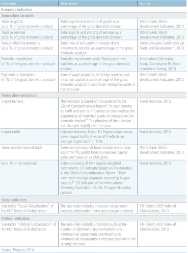
In order to quantify the economic effects of globalization the complex process that is globalization has to be made measurable first. This is done with the help of a comprehensive index which includes differentiated indicators that describe the economic as well as the political and social aspects of globalization (Table 1).2
The selected economic indicators are divided into two categories. The first category, “Transaction variables,” includes indicators that refer to actual transactions of goods, services or financial assets. A larger transaction volume indicates that a country is more strongly interconnected with the rest of the world. The category, “Transaction restrictions,” includes indicators for restrictions on the free transfer of goods and financial capital. Restrictions to transaction are a sign of a less globalized country. Both the social and political aspects of globalization are represented in the individual sub-indices of the KOF Index of Globalization.3
All in all, the selected indicators depict the process of globalization very well with regard to the depth and breadth of the sub-aspects under consideration. In order to achieve a comprehensive picture of globalization, the indicators must be compiled into an index.
2 Indicator selection is based on the KOF Index of Globalization, see Dreher (2006).
To this end, the data is first adjusted for outliers and then normalized to a standardized measure between 0 and 100.4
[image:11.595.58.428.213.709.2]4 To correct for oultiers, the manifestations of an indicator that lie below the 5 percent quantile and above the 95 percent quantile for this indicator are revised to the upper or lower limits for this quantile.
Table 1: Utilized globalization indicators
Indicators Description Source
Economic indicators Transaction variables Trade in goods
(as a % of gross domestic product)
Total exports and imports of goods as a percentage of the gross domestic product.
World Bank, World Development Indicators, 2013 Trade in services
(as a % of gross domestic product)
Total exports and imports of services as a percentage of the gross domestic product.
World Bank, World Development Indicators, 2013 Foreign direct investments
(as a % of gross domestic product)
Total inward and outward foreign direct investments (stocks) as a percentage of the gross domestic product.
United Nations Conference on Trade and Development, 2012
Portfolio investments
(in % of the gross domestic product) Portfolio investments stock: Total assets and liabilities as a percentage of the gross domestic product.
International Monetary Fund, Coordinated Portfolio Investment Survey, 2013 Payments to foreigners
(in % of the gross domestic product) Sum of wage payments to foreign workers and return on capital as a percentage of the gross domestic product. Income from intangible assets is not captured.
World Bank, World Development Indicators, 2012
Transaction restrictions
Import barriers This indicator is based on the question in the Global Competitiveness Report: “In your country, do tariff and non-tariff barriers to trade reduce the opportunity of imported goods to compete on the domestic market?” The phrasing of the question has changed slightly over the years.
Fraser Institute, 2013
Import tariffs Indicator between 0 and 10. Higher values mean lower import tariffs. A value of 0 reflects an average import tariff of 50%.
Fraser Institute, 2013
Taxes on international trade Taxes on international trade include import and export tariffs, profits from monopolies, capital gains and taxes on capital gains.
World Bank, World Development Indicators, 2013
(as a % of tax revenues) Index consisting of two equally weighted components. (1) Indicator based on the question in the Global Competitiveness Report: “How common is foreign corporate ownership in your country?” (2) Indicator of the International Monetary Fund that includes 13 types of capital controls.
Fraser Institute, 2013
Social indicators
Sub-index “Social Globalization” of the KOF Index of Globalization
The sub-index includes indicators on personal contacts, information flows and cultural proximity.
ETH Zurich, KOF Index of Globalization, 2013 Political indicators
Sub-index “Political Globalization” of
the KOF Index of Globalization The sub-index includes indicators such as the number of diplomatic representations and international agreements, membership in international organizations and participation in UN security missions.
ETH Zurich, KOF Index of Globalization, 2013
Higher values mean “more globalization” in each instance. 5 The correction for outliers is justified due to technical reasons as well as reasons that relate to the objective of the study: With respect to the latter, not every extreme event is an expression of globalization6; and technical, because outliers lead to distorted values after indicators are normalized.
In the next step, the econometric indicators are first compiled into a sub-index. This is done separately for the indicators in the two categories, transaction variables and transaction restrictions. Principal component analysis is applied as a statistical weighting which investigates the possible linear combinations of the individual indicators and selects the weighting factors such that the variance of the weighted sum of all indicators is maximized. This way the principal component analysis maximizes the statistical power of the resulting index. The resulting sub-indices for both categories are assigned equal weights when forming the sub-index that relates to the economic facet of globalization.7
Subsequently the three sub-indices are aggregated into a globalization index. Here the economic sub-index is assigned a weight of 60 percent while the social as well as political sub-indices are weighted at 20 percent. This intentional specification reflects the idea that the economic facets of globalization are considered most important when it comes to economic development. Thus, the disproportionate weighting of the economic components should always be seen as linked to the objectives of this study and does not represent a general value judgment concerning the significance of the individual components for globalization.
Some of the time series used exhibit data gaps. Missing values are treated as follows: Gaps in the midst of a series are linearly interpolated. The most recent available data points substitute for missing values at the beginning or end of a time series. If an indicator is not available for a country for the entire period of time, the entire series is imputed using regression analyses. To this end, an indicator is explained through all other utilized indicators in an auxiliary regression analysis. Knowledge about the explanatory power and manifestations of the existing indicators enables us to approximate the indicator that is unavailable.
Step 2: Studying the interrelated effects
The goal of this process step is to quantify the effect of globalization on growth using regression analysis. This enables us to filter out the effect of individual influencing variables on economic growth by statistically controlling for the effects of other explanatory variables of economic development.
5 The following formula is used to normalize indicators for which rising values indicate „more globalization.“ (Xj,t – Min(X))/ (Max(X) – Min(X)) * 100. The variable Xj,t is the individual manifestation of the indicator for the country j at time t. Max(X) and Min(X) are the maximum and minimum of this indicator for all countries and points in time. The following formula is used to normalize indicators for which rising values indicate „less globalization.“ (Max(X) – Xj,t)/(Max(X) – Min(X)) * 100.
In the regressions, economic development is operationalized through the growth of economic output per capita in percent. The specifically designed globalization index serves as the central explanatory variable. The regression results for this variable indicate the extent to which economic development is driven by globalization. In light of the importance of globalization for a domestic economy’s performance, we anticipate a positive and statistically significant effect for this variable.
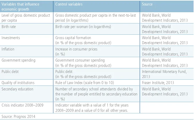
To ensure that the influence of globalization is neither overestimated nor underestimated, further determinants of economic development must be taken into account (Table 2). The anticipated growth effects of these variables are based on both theoretical considerations and empirical findings:
• The level of the gross domestic product per capita is considered in light of the theory of economic convergence.8 This theory states that domestic economies with a low gross domestic product per capita tend to display a higher rate of economic growth, which indicates a negative effect of this determinant.
• A higher birth rate has the short-term effect of distributing a given economic growth across a larger population base. Accordingly, we anticipate that higher birth rates correspond to smaller growth of economic output per capita.9
• By contrast, a positive on economic growth per capita can be assumed with regard to investment activities (private and public) because as a determinant of capital stock investments contribute substantially to the potential of national economies.
• The inflation rate serves as an indicator of macroeconomic stability. A low inflation rate is believed to stimulate economic activity, while a high inflation rate can counter overheated economic growth. Based on these considerations, we expect inflation to have a negative impact on economic growth.10
• Government spending as well as the debt ratio are considered key indicators of fiscal policy. While in terms of neoclassical theory and empirical findings we can assume that a high debt ratio is related to a reduction in economic growth, the influence of government spending is ambiguous a priori.11 On the one hand, high government spending can crowd out private investment activity. On the other hand, consumptive public spending can generate additional demand, promoting private investment.
8 The gross domestic product per capita is entered in the regressions with its values delayed by two years to prevent the economic growth per capita as an independent variable being used partially to explain itself.
9 Over the long term, a high birth rate can have positive effects on economic growth. However, such effects are not the subject of this study.
10 Theoretically, this is not necessarily the case. Negative inflation rates (deflation) can be expected to exert negative effects on growth. However, in this analysis, with the exception of Japan, deflation phases are of minor importance.
• Additionally, we control for the quality of the legal system with the Rule of Law Index. A highly developed legal system is considered an important prerequisite for strong economic growth.
• Secondary education as a proxy for human capital should have a positive impact on economic growth.
• We further control for the global economic crisis of 2008 and 2009 using an indicator variable.
The regression analysis includes all 42 countries contained in the Prognos World Report and addresses the period between 1992 and 2011.12 Therefore, 20 data points are available for each country and each variable. This data structure is taken into account by means of specific panel regression models.13
Bei der genauen Spezifikation des Regressionsmodells müssen zwei potenzielle Problemquellen berücksichtigt werden: unbeobachtete Heterogenität und die mögliche Endogenität verschiedener Einflussgrößen.
In the specification of the regression model, two potential problem sources need to be taken into account: unobserved heterogeneity and possible endogeneity of different explanatory variables.
12 Since the gross domestic product per capita is used in the regressions with its values delayed by two years, the data used for the regressions refers to the period of time between 1990 and 2011.
[image:14.595.171.541.297.524.2]13 All analyses were performed with the Stata 12 statistics program.
Table 2: Variables with a potential influence on economic growth as control
variables for the regression analysis
Variables that influence economic growth
Control variables Source
Level of gross domestic product per capita
Gross domestic product per capita in the next-to-last period (in logarithms)
World Bank, World Development Indicators, 2013 Birth rate Birth rate per woman (in logarithms) World Bank, World
Development Indicators, 2013 Investments Gross capital formation
(in % of the gross domestic product) World Bank, World Development Indicators, 2013 Inflation Increase in consumer prices
(in %) World Bank, World Development Indicators, 2013 Government spending Government consumer spending
(in % of the gross domestic product) World Bank, World Development Indicators, 2013 Public debt Public debt
(in % of the gross domestic product) International Monetary Fund, 2013 Quality of institutions Rule of Law Index (scale from 0 to 10) Fraser Institute, 2013 Secondary education Number of secondary school attendants divided by
the number of people entitled to secondary education (in %)
World Bank, World Development Indicators, 2013
Unobserved heterogeneity is based on the circumstance that even a careful selection of determinants cannot ensure that all differences between the countries under consideration are adequately accounted for. If these unobserved characteristics correlate with neither the dependent variable nor the control variables under consideration, no complication arises. If this does not apply, unobserved heterogeneity becomes a problem because the explanatory power of unobserved characteristics may falsely be assigned to other determinants. Thus, unobserved heterogeneity can result in distorted estimates for all determinants. For this reason, fixed effects models were used in the analysis. These control for differences between the countries that can assumed to be approximately constant over the observed period of time.14
Endogeneity problems can, e.g., occur when interdependencies exist between the dependent variable and one or more determinants. This type of connection can, e.g., be surmised for investment activities and economic growth: Strong investment activities encourage economic growth (and constitutes part of it) while, at the same time, positive economic development leads to a positive investment climate. In such cases, the difficulty arises in that we cannot differentiate which changes in the determinant influence the dependent variable and which changes result from reverse causality. Endogeneity problems also lead to distorted results.
To account for potential endogeneity problems, instrumental variable procedures (short: IV methods) are used. In this two-step process (also called a two-stage least squares estimation), each variable for which an endogeneity problem has to be suspected is divided into two parts: one part that is exogenous with respect to the dependent variable and one endogenous part. In the second step of the process – the actual regression – only the exogenous part of the original regressor is taken into account. This ensures that no endogeneity problems exist in the final regression. In order to apply this method, at least one instrumental variable is needed for each potential endogenous determinant. It must be highly correlated with the endogenous explanatory variable while simultaneously holding explanatory power for the dependent variable, but must not be affected by the same endogeneity problem.
In this study the time series of the potentially endogenous control variables are lagged by one year and then used as instrumental variables. Under the assumption that the dependent variable can be affected by current and past growth rates of the gross domestic product, but not by future realizations, these time series meet all requirements for suitable instrumental variables. Based on this approach, the assumption of exogeneity was discarded for the variables investment activity and birth rate. 15
14 We are testing the fixed effects model in a comparison with a simple OLS model (least squares estimation) The unrestricted fixed effects model contains one constant and 41 country-specific indicator variables. The restricted OLS contains only the constant. The LR test between the two models examines whether the implicit restriction of the country-specific indicator variables to the value 0 is justified. However, the test results refute this hypothesis. In this context, the fixed effects model seems to be the more convincing alternative.
The regression results with respect to the effects of globalization can be interpreted as follows: If the globalization index rises by one point, the growth of the gross domestic product per capita increases by b percentage points, whereby b equals the level of the estimated growth effect of globalization. An illustration: The economic growth per capita is 2.5 percent; the estimator for the effect of globalization is b=0.2. In this case, a rise in the globalization index of one point leads to an increase in economic growth from 2.5 to 2.7 percent. This relationship is constant for all observed countries and for the entire study period.
This knowledge of the sensitivity of economic growth per capita with regard to globalization is used in the next step to quantify the globalization-induced growth gains for the individual countries.
Step 3: Determining the „globalization champion”
The quantification of globalization-induced growth gains involves two steps:
• In the first step, we calculate for each country which growth rates would have resulted from a stagnation in the level of globalization. To this end, annual changes in the globalization index are multiplied by the estimator for the globalization-induced growth effect and subtracted from the historical series of growth rates.
• Starting with the gross domestic product at the beginning of the study period and using the newly calculated growth rates a counterfactual growth trajectory can be constructed for each country that depicts the economic course if the globalization had been stagnant.
The comparison of the historical series of the gross domestic product and those that result from counterfactual growth path enables us to tabulate and compare the globalization-induced growth gains and losses for the individual countries. The “globalization champion” is determined according to the highest globalization-induced gains in income per capita between 1990 and 2011.
2.1.2 Scenarios for future globalization developments
The scenario calculations aim to demonstrate the significance that increasing global interconnectedness may have for future economic developments. To this end, two independent scenarios were devised.
2011 increase their pace of globalization more strongly in this scenario than those countries with a relatively high speed of globalization. The scenario parameter thus implies a realistic catching-up process for countries that were only able to achieve a rather weak globalization progress over the last two decades.
In the “diverging globalization” scenario, globalization comes to a stop in the euro countries Greece, Portugal and Spain. This scenario demonstrates the hidden risks that result for these countries solely through stagnation of their level of interconnectedness with the rest of the world.
Both scenarios are implemented using the global macroeconomic model VIEW by Prognos (Box 1). Predictions from the Prognos World Report 2013 serve as the starting point for the scenario calculations. These baseline projections play a key role by setting an anchor point as the “most likely scenario” or reference development. It thus constitutes the basis for simulating changes resulting from the scenario parameters. The implicit assumption that the baseline projection is compatible with a “normal globalization development” is justified because no breaks are assumed in the globalization dynamic for this reference development, but rather the most probable courses for all facets of economic development.
Box 1: VIEW, the global economic model by Prognos
VIEW is a comprehensive macroeconomic model. It includes the origin and use of goods and services as well as the labor market and public finances, and systematically connects all participating countries through exports, imports, exchange rates, etc.
This global forecasting and simulation model allows for a consistent and detailed representation of future developments of the global economy. Interactions and feedback between individual countries are captured and modeled explicitly in VIEW. For that reason, its analytical meaningfulness goes far beyond the isolated country models with exogenous defined parameters for the global economic system. In its current version, VIEW includes the 42 most important countries in the world based in terms of economic output – and thus over 90 percent of the global economic output.
The different globalization developments are simulated through their impacts on foreign trade dynamics. Here the most important variable is the growth rate of the imports of goods. In each scenario this variable is specified in terms of its deviation from the baseline projection according to the conception of the scenario.16 By contrast, the growth rate of the exports of goods in each scenario results from the changes in imports t and the international trade relationships which are taken into account for in the model.17 Foreign trade does not just model one of the most significant channels of the effects of globalization on economic development. Because of the detailed representation of bilateral trade relationships in VIEW, foreign trade is optimally suited in the model for representing and analyzing the complex effects of increasing worldwide integration.
The specific implementation of the stipulated development of globalization in each of the scenarios accounts for the historical development of the level of imports and its interaction with the development of the globalization index:
• For the “accelerated globalization” scenario, in a first step the average yearly increase of the globalization index is calculated for all countries between 1990 and 2011. Half of this value constitutes the scenario parameter regarding the absolute acceleration of globalization. This is the same for all countries.18 To determine its influence on each country’s foreign trade, ex-post data is used to determine the change in growth for a country’s goods imports. To this end, the average growth rate of the imports of in the ex-post time period is set in relation to the average annual difference of the globalization index and finally multiplied by the scenario parameter for accelerated pace of globalization.
• Parameters for the “diverging globalization” scenario only affect Greece, Portugal and Spain for which globalization is assumed to stagnate. To model this development, the annual growth rates of goods imports for each country are set in relation to the average annual changes in the globalization index. The results in this calculation indicate the degree to which the increasing globalization in each individual country is accompanied by a change in goods imports. Since the scenario aims to model stagnation in the degree of integration and the baseline forecast is assumed to be reconcilable with normal globalization development in a historical context, the scenario parameters for the growth rates of goods imports can be determined as the difference between the growth rates in the baseline forecast and the globalization-related growth rates calculated as described.
16 At this point, we intentionally refrain from exogenizing imports of both goods and services. Contentwise no major differences would be expected in the results for the scenario calculations since imports of goods make up more than 90 percent of total imports for almost every country under consideration. Technically, this approach is imperative because each exogenous implementation requires a modification of the model’s logic.
17 A simultaneous exogenization of exports and imports of goods would not be compatible with the international trade networks that are considered in the model. Such an approach would disregard significant features of global economic interconnections and thus not lead to meaningful results.
2.2 Globalization index: results
This section initially presents the results of the descriptive analysis of the globalization index. Building on that, the regression results are analyzed with regard to the interrelated effects between globalization and growth of the gross domestic product. Finally, a globalization champion is determined based on globalization-induced income gains.
2.2.1 Descriptive analysis of the globalization index
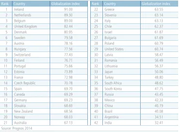
The analysis of the globalization index shows that highly-developed, well-integrated national economies that tend to be smaller exhibit especially high manifestations of the globalization level as Ireland, the Netherlands and Belgium place themselves on the top of the rankings (Table 3).
[image:19.595.57.429.354.626.2]In contrast, larger and highly-developed countries such as Germany, France, Italy and Spain rank at mid-table. Noteworthy in this context is the comparatively high position of the United Kingdom. Major developing nations such as China, Brazil and India place themselves mainly toward the bottom of the globalization index. These results are thus comparable with the results of other globalization indices (Box 2).
Table 3: Globalization index for the year 2011
Rank Country Globalization index Rank Country Globalization index
1 Ireland 91.00 22 Greece 63.55
2 Netherlands 89.30 23 Slovenia 63.14
3 Belgium 89.00 24 Italy 63.13
4 United Kingdom 82.44 25 Chile 62.37
5 Denmark 80.95 26 Israel 61.87
6 Sweden 79.58 27 Bulgaria 61.69
7 Austria 78.16 28 Poland 60.79
8 Hungary 77.56 29 United States 60.74
9 Switzerland 77.43 30 Latvia 58.47
10 Finland 76.71 31 Romania 56.49
11 Portugal 75.66 32 Lithuania 56.37
12 Estonia 73.89 33 Japan 50.06
13 France 72.98 34 Turkey 48.80
14 Czech Republic 70.78 35 South Africa 48.62
15 Spain 69.70 36 South Korea 47.75
16 Canada 69.29 37 Russia 43.45
17 Germany 69.23 38 Mexico 42.33
18 Slovakia 68.60 39 China 40.19
19 New Zealand 68.56 40 Brazil 40.08
20 Norway 68.03 41 Argentina 34.51
21 Australia 67.13 42 India 32.41
Box 2: Comparison of the globalization index with the New
Globalization Index19, the Globalization Index of Ernst & Young and the
Economic Intelligence Unit (EIU)20, and the KOF Index of Globalization.21
In the comparison of the different globalization indices, index rankings were limited to the list of countries considered in this study (Table 4). At first the comparison reveals many commonalities. Small, highly-developed nations such as the United Kingdom ranked near the top in all indices under consideration. Large and highly-developed national economies such as Germany, France, Italy, Canada and Spain place themselves in the middle of the ranking. In contrast, the United States and Japan are ranked at the bottom end of the midrange in all indices. The last places in the globalization indices are held consistently by major developing nations.
But the comparison of the indices also revealed differences. The average absolute deviation in the ranking positions between the globalization index used in this study and the New Globalization Index amounts to 4.2 places. The corresponding values for the Globalization Index of Ernst & Young/EIU and the KOF Index of Globalization amount to 3.6 and 2.2 places, respectively. The relatively large deviations in the New Globalization Index are due to an older data set from 2005 and due to the fact that all trade flows were weighted with the distance to the individual trade partner for this index. This approach causes global trade to be weighted more heavily than regional trade which improves the ranking position for Argentina and South Africa for example but worsens that of Hungary and the Czech Republic. In regard to the Ernst & Young/EIU index, the differences essentially arise as the result of differences in the indicators considered and the weighting procedure. The Ernst & Young/EIU, e.g., index takes into account the mobility of the labor force which is not the case in the index used for this study. Conversely, the political aspects of globalization are not considered in the index from Ernst & Young/EIU, which places comparatively well-integrated countries such as Austria, Portugal and Turkey at a disadvantage. Deviations from rankings in the KOF Index of Globalization are comparatively small which is not surprising due to the conceptual similarities to the globalization index utilized in this study. Different weighting of the sub-indices mainly results in differences for Estonia, which received a comparatively higher value for the economic sub-index leading to an improved ranking position in the index used here.
19 See Vujakovic (2010).
20 See Ernst & Young (2013). The index from Ernst & Young/EIU is based on a survey of business experts from the year 2012, supplemented by data from government statistics.
Table 4: Differences between the globalization index and other indices with
regard to rankings
Rank in the
globali-zation index Country New Globalization Index Ernst & Young, EIU KOF Index of Globalization
1 Ireland 0 0 –1
2 Netherlands 0 –1 0
3 Belgium –2 0 1
4 United Kingdom 0 –3 –5
5 Denmark –2 0 1
6 Sweden –3 –1 –2
7 Austria 3 –8 5
8 Hungary –15 1 0
9 Switzerland 5 4 –2
10 Finland –4 0 –2
11 Portugal –10 –17 3
12 Estonia 1 – –10
13 France 1 0 –2
14 Czech Republic –8 –2 2
15 Spain –2 –3 1
16 Canada 7 2 5
17 Germany 4 9 –1
18 Slovakia 6 9 3
19 New Zealand 4 1 –4
20 Norway 7 –4 0
21 Australia 3 –1 3
22 Greece –5 –8 4
23 Slovenia –3 – 0
24 Italy 3 –4 4
25 Chile –2 –3 –6
26 Israel 4 8 –2
27 Bulgaria 0 7 –4
28 Poland 0 4 5
29 United States 4 6 2
30 Latvia –4 – –2
31 Romania –11 1 0
32 Lithuania – – 3
33 Japan –6 –2 –3
34 Turkey –8 –4 2
35 South Africa 9 –5 0
36 South Korea –2 6 –1
37 Russia 3 –2 3
38 Mexico 2 5 0
39 China 7 2 0
40 Brazil 0 3 0
41 Argentina 8 0 0
42 India 6 0 0
Note: The difference in a country‘s ranking position is calculated as the country‘s ranking position in the globalization index used in this study minus the ranking position in the respective comparison index. “–“ indicates that the country in question is not considered in the individual index.
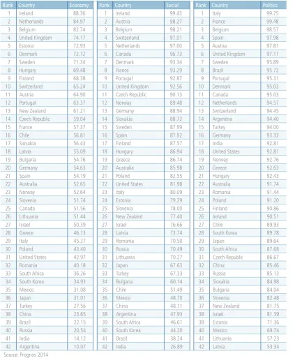
A glance at the sub-indices gives an indication of how the ranking in the overall index should be evaluated (Table 5). For example, the leading positions of Ireland, the Netherlands and Belgium result from high values in the economic and social sub-indices. But the three front runners also post high values in the political sub-index, even though other countries hold the top places here.
At first, the low globalization index values for major developing nations may seem surprising, but they are reflected consistently in the poor positions for these countries in the economic and social sub-indices.22 One reason for this result is the normalization of total transaction volumes in the economic sub-index with the size of the respective economy (Box 3).23
Box 3: China’s position in the globalization index
China ranks 39th in the overall index. This result is largely determined by China’s low position in the economic sub-index. What may seem surprising in light of China’s importance for the global economy can be explained with a look at China’s values for the individual indicators:
First, we need to bear in mind that the economic sub-index not only incorporates transaction volumes, but also other indicators that measure the restrictions on transactions. Due to its restrictive trade policy, China finishes at the end of the set here for all four indicators. This is most pronounced for the capital controls indicator. With 3.0 out of 10 points, China shows the third-lowest value for this indicator among all observed nations. For comparison: Frontrunners in the globalization index like Ireland or the Netherlands exhibit values between 8 and 9 points.
Second, China does not show particularly favorable values for indicators in the “transaction volumes” category in comparison to other national economies. This applies to portfolio investments (10.5 of the gross domestic product and rank 38) as well as foreign direct investments (15 percent of the gross domestic product and rank 42) and trade in services (6 percent of the gross domestic product and rank 39). Even in trade in goods (46 percent of gross national product) China only achieves 29th place among all countries under consideration. One important reason for this finding is that, for the globalization index, the absolute transaction volumes of a country are normalized with the gross domestic product. With respect to trade in goods, China, e.g., ranks in second place behind the United States with an absolute value of over €2.4 billion, which is five times as high as that of Belgium. If
we consider these numbers as percentage values in relation to the gross domestic product of the individual nation, Belgium achieves values nearly three times as high as China.
22 To a minor extent this also applies to the political sub-index.
Table 5: Sub-indices of the globalization index for the year 2011
Rank Country Economy Rank Country Social Rank Country Politics
1 Ireland 88.36 1 Ireland 99.43 1 Italy 99.75
2 Netherlands 84.97 2 Austria 98.27 2 France 99.48
3 Belgium 82.74 3 Belgium 98.21 3 Belgium 98.57
4 United Kingdom 74.17 4 Switzerland 97.01 4 Spain 97.98
5 Estonia 72.93 5 Netherlands 97.00 5 Austria 97.81
6 Denmark 72.12 6 Canada 96.73 6 United Kingdom 97.11
7 Sweden 71.34 7 Denmark 93.34 7 Sweden 95.89
8 Hungary 69.48 8 France 93.29 8 Brazil 95.72
9 Finland 68.38 9 Portugal 92.87 9 Portugal 95.31
10 Switzerland 65.24 10 United Kingdom 92.56 10 Denmark 95.03
11 Austria 64.90 11 Czech Republic 90.13 11 Canada 95.03
12 Portugal 63.37 12 Norway 89.48 12 Netherlands 94.57
13 New Zealand 61.21 13 Germany 88.94 13 Switzerland 94.45
14 Czech Republic 59.04 14 Slovakia 88.72 14 Argentina 94.40
15 France 57.37 15 Sweden 87.99 15 Turkey 94.00
16 Chile 56.81 16 Spain 87.92 16 Germany 93.33
17 Slovakia 56.43 17 Finland 87.57 17 India 92.81
18 Latvia 55.09 18 Hungary 86.94 18 United States 92.81
19 Bulgaria 54.76 19 Greece 86.74 19 Norway 92.76
20 Germany 54.63 20 Australia 85.98 20 Greece 92.63
21 Spain 54.19 21 Poland 82.55 21 Hungary 92.43
22 Australia 52.65 22 United States 81.98 22 Australia 91.74
23 Norway 52.64 23 Italy 80.09 23 Romania 91.44
24 Slovenia 51.74 24 Estonia 79.29 24 Poland 91.20
25 Canada 51.56 25 Slovenia 78.00 25 Finland 90.86
26 Lithuania 51.44 26 New Zealand 77.40 26 Ireland 90.51
27 Israel 50.39 27 Israel 76.66 27 Chile 89.93
28 Greece 46.13 28 Latvia 73.74 28 South Korea 89.78
29 Italy 45.27 29 Romania 70.50 29 Japan 89.64
30 Poland 43.40 30 Russia 70.49 30 South Africa 87.68
31 United States 42.97 31 Lithuania 70.27 31 Czech Republic 86.67
32 Romania 40.18 32 Japan 67.63 32 China 85.46
33 South Africa 36.26 33 Turkey 67.33 33 Russia 85.13
34 South Korea 34.93 34 Bulgaria 60.14 34 Slovakia 84.98
35 Mexico 31.08 35 Chile 51.49 35 Bulgaria 84.04
36 Japan 31.01 36 Mexico 48.70 36 Slovenia 82.48
37 Turkey 27.56 37 China 48.11 37 New Zealand 81.75
38 China 23.65 38 Argentina 47.93 38 Israel 81.39
39 Brazil 22.15 39 South Africa 46.61 39 Estonia 71.36
40 Russia 20.54 40 South Korea 44.20 40 Mexico 69.74
41 India 14.12 41 Brazil 38.24 41 Lithuania 57.23
42 Argentina 10.07 42 India 26.89 42 Latvia 53.34
Highly-developed national economies that place themselves at mid-table of the overall index take on leading positions in the political sub-index. This applies in particular to Italy, France and Spain, and to a lesser extent to Germany. In the social index and particularly in the economic sub-index, these countries rank mostly at mid-table. In particular, Germany, despite being a global export champion for a long time, only achieves middle-of-the-road ranking throughout. Germany’s distance from the pack leaders, as measured in index points, is especially significant in the economic sub-index.
To be able to better classify a few sub-aspects of these results, it is illustrative to visualize the country-specific differences for a few indicators. However, when interpreting the manifestations of the individual indicators, we must keep in mind that high or low values are not necessarily associated with an implicit value judgment. However, as a gauge for sub-aspects of the integration of individual countries with the rest of the world, they hold decisive explanatory power for the ranking in the overall index or the sub-indices.
For example, Germany‘s relatively low value on the globalization index can at least be partially explained by scale effects. In 2011, the total of exports and imports of goods was around €2 billion
and therefore four times as high as that of Belgium. This order is reversed when viewed in relation to the gross domestic product: Belgium imported and exported goods at a value of around 128 percent of its economic output. This degree of openness is around 77 percent for Germany. Similar relationships exist for other economic indicators as well.
A further reason for the leading positions of Ireland, the Netherlands and Belgium and Germany’s comparatively poor performance lies in geographic circumstances and financial market structures. For example, the Netherlands and Belgium have very high foreign trade levels partly because of their well-developed port infrastructures. By contrast, Ireland exhibits an astronomical 1,300 percent in portfolio investments in relation to its gross domestic product. Ireland also occupies a leading position in foreign direct investment, which is nearly 261 percent of its gross domestic product. By comparison, Germany merely displays values of 143 and 60 percent, respectively, in these areas. In the same context, the United Kingdom’s high figure in the economic sub-index reveals that it benefits in this ranking from London as a strong financial center.
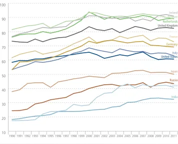
With this we can state that, particularly smaller but highly-developed national economies are among the most globalized countries in the world. These countries owe their ranking in part to their economic indicator figures, which are high in relation to economic output. With the exception of the United Kingdom, the European core states occupy places in the middle range, an outcome essentially caused by the moderate values of the economic indicators and further strengthened by the heavy weighting of this sub-index. The major developing nations form the group at the bottom of the globalization index, but exhibit greater dynamics over time.
[image:25.595.57.414.192.479.2]Source: Prognos 2014
Figure 1: Manifestations of the globalization index for selected countries from
1990 to 2011
10 20 30 40 50 60 70 80 90 100
United Kingdom
United States
Russia
Netherlands
Japan
Italy Ireland
India
France
Germany
China
Belgium
2.2.2 Regression analyses on the relationship between globalization and economic growth
The following discussion of the regression results for the growth effects of globalization focuses on our baseline specification (Table 6, Column 2). In addition to the globalization index as the main explanatory variable, this specification includes the gross domestic product per capita, the birth rate, investments and a crisis indicator for the years 2008 and 2009 as control variables.24
The results verify that globalization has a significantly positive influence on gross domestic product per capita growth. The estimated coefficient of 0.35 indicates that an increase of the globalization index by one point on average leads to an increase in growth rate of the gross domestic product per capita by 0.35 percentage points. This, e.g., suggests that with an average rise in the globalization index of 0.76 points per year between 1990 and 2011, Germany owes 0.27
24 The selection of variables for the baseline specification is based largely on the significance of the effects on growth of these determinants as indicated by the results. Additionally, the two endogenous control variables – investments and fertility – are included to enable comparable results across all specifications..
Table 6: Regression results regarding the determinants of economic growth per
capita
Dependent variable: Growth of the gross domestic product per capita as a percent
IV method with FE IV method with FE and country groups
Total globalization 0.35*** –
(0.07) Globalization for
Large national economies with a high per capita income – 0.26*** (0.05) Small national economies with a high per capita income – 0.26***
(0.06) Large national economies with a low per capita income – 0.29
(0.16) Small national economies with a low per capita income – 0.40***
(0.10) Gross domestic product per capita in the next-to-last period
(logarithmized)
–10.48*** –10.02***
(1.60) (1.70)
Birth rate (logarithmized) –10.44*** –10.19**
(2.42) (3.26)
Investments (as a % of the gross domestic product) 0.15 0.12
(0.10) (0.10)
Crisis indicator 2008-–009 –3.55*** –3.59***
(0.43) (0.43)
Number of observations R² (centered)
840 840
0.40 0.40
Notes: The symbols *, **, *** indicate the significance of the estimation results for the 10%, 5% and 1% levels. Standard errors are clustered by country and displayed in parentheses. All regressions contain a constant. FE is the abbreviation for country-specific fixed effects.
percentage points of its annual per capita growth to its increasing interconnectedness with the rest of the world.
This figure equals almost 20 percent of the average growth of the gross domestic product per capita in the same period of time, which signals the decisive importance that can be attributed to globalization alongside other drivers of growth such as technological progress.
The other estimated results of the baseline specification show the expected signs. The gross domestic product per capita, the birth rate and the indicator for the most recent global economic crisis are included with minus signs in the estimation equation. Also, all of them are statistically significant. A coefficient of -10.48 for the influence of economic output means that a 1 percent increase in the gross domestic product per capita leads to a reduction of per capita growth of 0.105 percentage points two years later. Similarly for fertility, a 1 percent increase corresponds to a 0.105 percentage point decline in growth per capita. The estimated 3.55 coefficient for the crisis years 2008 and 2009 signifies that the economic growth per capita during this period was approximately 3.5 percentage points lower than in the rest of the observation period. At 0.15, the estimated value for investments in relation to the gross domestic product also exhibits the expected sign, but is not statistically significant.25
The reliability of estimated results is checked using a variety of alternative regression specifications. As the first alternative, we consider a specification in which the growth effect of globalization is estimated separately for different country groups, but in which the same explanatory variables are taken into account. To this end, the countries under consideration are separated into four groups of approximately equal size based on the gross domestic product per capita in the year 1990 and the size of the economy, as measured by the gross domestic product of the same year (Table 7).26
The results demonstrate that all four country groups exhibit similar sensitivities in per capita growth with regard to globalization (Table 6, Column 3). At 0,40, small national economies with a low gross domestic product per capita show a slightly greater sensitivity in economic growth with regard to globalization, while all other country groups display a slightly lower sensitivity. Differences between the estimators are too small to allow meaningful interpretations, as none of the estimators differ significantly from 0.35.27
25 Estimators that do not signal a statistically significant effect of investments on the gross domestic product are not uncommon in the empirical literature. See Dreher (2006) and Borys, Polgár, & Zlate (2008).
26 The division was performed as follows: First, all countries being studied were separated into two groups according to a median split with respect to the gross domestic product per capita in the year 1990. This figure amounted to €10,050. Next, the country
groups formed in this way were each divided into two sub-groups based on the median split according to the gross domestic product in the year 1990. This figure amounted to €250 billion for the group of countries with a high gross domestic product per
capita and €95 billion for the group of countries with a low gross domestic product per capita.
This result signals that alternative specifications with country-group-specific estimators for the growth effects of globalization do not come to meaningfully different conclusions. Furthermore, the estimated coefficients of the remaining explanatory variables hardly differ from those of the baseline specification.
As alternative specifications, additional regressions with different combinations of explanatory variables were run using both the baseline specification as well as the specification with country-group-specific sensitivities as starting points.28 Results of these regressions corroborate the finding that both the estimated effects of globalization on growth as well as those of the remaining explanatory variables are robust and can be considered reliable (Table 33 and Table 34 in Appendix A).29
The overall result of the regression analyses documents the stable and significant positive influence of globalization on per capita growth. In particular, the high reliability of the estimations strengthens the confidence in the regression results. For that reason, the estimated sensitivity of per capita growth in the baseline specification of 0.35 percentage points for each point of the globalization index can be considered a key interim result of this section. The „globalization champion” will be determined in the next section based on this sensitivity.
28 Furthermore, the terms of trade were taken into account in additional regressions as a control variable for the relation of export to import prices. The results across all specifications exhibit a positive, but insignificant influence of the terms of trade on economic growth and no change of the estimated effect of globalization on growth.
29 Moreover, all explanatory variables are included in the estimation equation with the expected signs. The only exception is secondary education, for which the estimated effect turns out to be negative although the estimator fails to reach statistical significance at a conventional level.
Table 7: Classification of the national economies under consideration based on
the gross domestic product per capita and the size of the economy
Large national economies with a high per capita income
Small national economies with a high per capita income
Large national economies with a low per capita income
Small national economies with a low per capita income
Australia Belgium Argentina Bulgaria
Germany Denmark Brazil Chile
France Finland China Estonia
Italy Greece India Latvia
Japan Ireland Mexico Lithuania
Canada Israel Poland Romania
Netherlands New Zealand Portugal Slovakia
Switzerland Norway Russia Slovenia
Spain Austria South Africa Czech Republic
United States Sweden South Korea Hungary
United Kingdom Turkey
2.3 Growth effects of globalization
This section aims to answer the question regarding the extent to which the countries under consideration have benefited from the ongoing globalization in the time period from 1990 to 2011. This analysis is based on the comparison of the historical development of the gross domestic product with a counterfactual scenario for which globalization is assumed to have stagnated at the level prevailing at the outset of the observation period. In other words: We assume in the scenario that the globalization index in all the years from 1991 to 2011 remained fixed at the 1990 level for the each country.30 We use the differences in the development of the gross domestic product per capita, summed up over the entire observation period, as the basis for measuring globalization gains. When interpreting the results, we must distinguish between economic growth and cumulative income gains (Box 4).
The country whose residents have benefited the most from increasing globalization will be crowned the „globalization champion.” In accordance with the economics focus of the study, both the absolute income gains per capita and the per capita income gains weighted according to purchasing power are used as two alternative indicators to determine the “globalization champion.”
For a differentiated representation of the results with regard to the different starting positions and proportions of the national economies, we utilized the globalization-induced income gains per capita in relation to the value of the gross domestic product in the year 1990 as well as the aggregated income gains of the entire national economy. In order to also convey an impression of the extent to which global integration tendencies are associated with changes in the distribution of net household income, we subsequently compare the globalization-induced income gains with the changes in the Gini coefficients for the individual countries.
Box 4: Interpreting the globalization-induced income gains as an indicator for determining the „globalization champion”
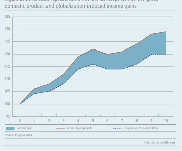
The assumed stagnation of globalization causes low economic growth and thus an unfavorable growth path. The yearly difference between the level of the gross domestic product per capita according to this alternative path and the actual development shows the absolute economic gains (Figure 2).
30 The development of the gross domestic product per capita is calculated with the following formula for the counterfactual scenario:
!"#! !"!!=
!"#!""# !"!!""#∗ 1 +
!!− 0,35 ∗ (!"!− !"!!!) 100 !
!!!""!
These gains for each country under consideration are summed up for the entire time period of 1990 to 2011 as a measure for the cumulative effects of globalization. In this study, the variable calculated in this way will be designated as the “cumulative income gain induced by progressing globalization.” This variable should not be confused with variables that are used in the system of national accounts, such as the available income.
Furthermore, we must distinguish between cumulative income gains and changed growth rates. For example, even a one-time higher growth rate of the gross domestic product induces income gains that accumulate over the remaining study period, even when growth rates in the remaining time frame remain unchanged. By contrast, a one-time globalization-related income gain has no implications for the growth rate in the following years.
[image:30.595.173.534.332.631.2]Source: Prognos 2014
Figure 2: Schematic representation of the development of the gross
domestic product and globalization-induced income gains
actual development stagnation of globalization
95 100 105 110 115 120 125 130 135
10 9 8 7 6 5 4 3 2 1 0
2.3.1 Determining the „globalization champion” based on income gains per capita
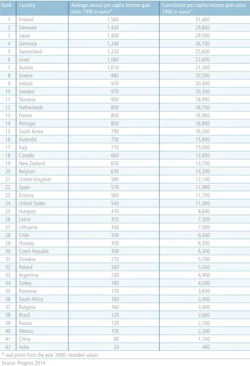
Considering the absolute income gains per capita resulting from increasing globalization, we see that two Scandinavian nations occupy the first two places in the ranking (Table 8).31 According to this approach, Finland is the “globalization champion”, followed by Denmark. With Switzerland, Austria, Greece, Ireland and Sweden, five additional small European countries rank among the top ten. But some large national economies including Germany and Japan report large income gains per capita as well and, thus, can count themselves among the stronger beneficiaries of the globalization process.
Places 11 through 24 are occupied primarily by Central European countries or national economies with a gross domestic product per capita that is high in comparison with the rest of the world. Slovenia, South Korea and Estonia are exceptions here. It is noteworthy that residents of large industrial nations do not benefit equally from the increasing interconnectedness in the world. Globalization gains per capita in the United Kingdom and United States are less than half as high as those for Germany, for example. Countries like Italy, Canada and Spain fall under this category as well. Reasons for this finding can be mainly found in the different developments of the globalization index. Germany benefits on the one hand in that it was able to post the greatest growth in the globalization index between 1990 and 2011 among the mentioned countries under (Table 28 through Table 32 in Appendix A).
Equally important is the fact that Germany’s progress with regard to integration with the rest of the world can be primarily attributed to the first half of the observation period. In comparison to many other national economies, globalization-related income gains in Germany were therefore able to accumulate over a longer period of time.
The lower mid-range of globalization winners is completed primarily by nations from Eastern Europe and the Baltic states. While these national economies were only able to achieve from 20 to 30 percent of the frontrunners’ globalization gains per capita, this can still be considered an impressive success especially in light of the economic turmoil after the fall of the Soviet Union.
The large developing nations rank last in the comparison of absolute globalization gains per capita. Therefore, in terms of absolute cumulative income gains per capita, they do not count to the strong beneficiaries of globalization, despite their significance for the world economy e which is due to their large domestic markets and highly dynamic economies.
Table 8: Absolute income gains per capita as the result of increasing
globalization in the period of time from 1990 to 2011
Rank Country Average annual per capita income gain
since 1990 in euros* Cumulative per capita income gain since 1990 in euros*
1 Finland 1,500 31,400
2 Denmark 1,420 29,800
3 Japan 1,400 29,500
4 Germany 1,240 26,100
5 Switzerland 1,220 25,600
6 Israel 1,080 22,600
7 Austria 1,010 21,300
8 Greece 980 20,500
9 Ireland 970 20,400
10 Sweden 970 20,300
11 Slovenia 900 18,900
12 Netherlands 890 18,700
13 France 800 16,900
14 Portugal 800 16,800
15 South Korea 790 16,500
16 Australia 750 15,800
17 Italy 710 15,000
18 Canada 660 13,800
19 New Zealand 650 13,700
20 Belgium 630 13,200
21 United Kingdom 580 12,100
22 Spain 570 11,900
23 Estonia 560 11,700
24 United States 540 11,300
25 Hungary 410 8,600
26 Latvia 350 7,300
27 Lithuania 330 7,000
28 Chile 300 6,400
29 Norway 300 6,300
30 Czech Republic 300 6,300
31 Slovakia 270 5,700
32 Poland 260 5,500
33 Argentina 230 4,900
34 Turkey 190 4,000
35 Romania 170 3,600
36 South Africa 160 3,400
37 Bulgaria 160 3,400
38 Brazil 120 2,600
39 Russia 120 2,500
40 Mexico 100 2,200
41 China 80 1,700
42 India 20 400
Another important finding emerges for those countries that exhibit the highest values for the globalization index: Neither Belgium, the Netherlands nor Ireland are among the top-ranked countries in terms of globalization gains per capita. The reason for this result is that, although these national economies have a high degree of integration with the rest of the world, they exhibited low momentum during the study period. This result clearly shows the importance of ongoing efforts to integrate national economies with the rest of the world, even for – or perhaps especially for – very globalized nations.
Observing the development over time sheds additional light on how the globalization-induced income gains per capita should be assessed (Figure 4 through Figure 7 in Appendix B). It shows that the strongest gains in terms of growth should be attributed to the period from the mid-1990s to the middle of the first decade of the 21st century. “Globalization champion” Finland and the other main beneficiaries from globalization were able to increase their gross domestic product per capita through globalization at the beginning of the study period. This makes clear how important the developments in the early years of the observation period are for the overall results of this study: The earlier a country was able to benefit from globalization, the longer the period of time during which the income gains per capita could be accumulated. The boom in technology and the important role of the Finnish telecommunications industry in the 1990s may therefore be decisive factors in the final ranking of the beneficiaries from globalization. By contrast, the selection of the observation period puts countries such as Chile or Slovakia, which were only able to achieve significant increases in the globalization index in the later on, at a disadvantage.
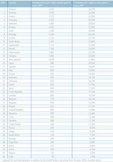
To what extend the situation has improved due to the ongoing globalization depends not only on the absolute income gains, but most notably on the level of consumption that individuals can afford as a result. For this reason, we analyzed income gains per capita that have been weighted according to purchasing power as an alternative way to determine the „globalization champion” (Table 9).
Table 9: Per capita income gains induced by increasing globalization in the
period of time from 1990 to 2011, adjusted for purchasing power
Rank Country Average annual per capita income gain in
euros, APP* Cumulative per capita income gain in euros, APP*
1 Finland 1,630 34,300
2 Slovenia 1,570 33,000
3 Greece 1,570 32,900
4 Germany 1,400 29,300
5 Denmark 1,360 28,600
6 Estonia 1,330 27,900
7 Israel 1,280 26,800
8 Portugal 1,240 26,100
9 Austria 1,220 25,700
10 South Korea 1,190 25,000
11 Switzerland 1,110 23,300
12 Ireland 1,100 23,000
13 Netherlands 1,080 22,700
14 Hungary 1,080 22,600
15 New Zealand 1,030 21,600
16 Japan 980 20,500
17 Sweden 970 20,300
18 Italy 950 19,900
19 France 930 19,500
20 Australia 910 19,100
21 Lithuania 870 18,300
22 Latvia 840 17,700
23 Spain 830 17,500
24 Czech Republic 810 17,100
25 Canada 800 16,700
26 Belgium 770 16,100
27 Bulgaria 630 13,300
28 Poland 620 13,100
29 United Kingdom 600 12,600
30 Romania 590 12,400
31 Chile 580 12,200
32 Slovakia 560 11,700
33 United States 540 11,300
34 Russia 450 9,500
35 Turkey 410 8,700
36 South Africa 370 7,700
37 Norway 290 6,100
38 Argentina 280 5,800
39 Brazil 230 4,900
40 China 200 4,100
41 Mexico 170 3,500
42 India 60 1,200