Integration of Lower Bound Estimates in Pseudo Boolean Optimization

Integration of Lower Bound Estimates in Pseudo-Boolean

Optimization

Vasco M. Manquinho and Jo˜

ao Marques-Silva

IST/INESC-ID, Technical University of Lisbon, Portugal

{

vmm,jpms

}

@sat.inesc-id.pt

Abstract

Linear Pseudo-Boolean Optimization (PBO) has found applications in several areas, ranging from Ar-tificial Intelligence to Electronic Design Automation. Due to important advances in Boolean Satisfiabil-ity (SAT), new algorithms for PBO have emerged, which are effective on highly constrained instances. How-ever, those algorithms fail in dealing properly with the objective function of PBO. This paper proposes an al-gorithm that uses lower bound estimation methods for pruning the search tree in integration with tech-niques from SAT algorithms. Moreover, the paper shows that the utilization of lower bound estimates can dramat-ically improve the overall performance of PBO solvers for specific classes of instances. In addition, the paper de-scribes how to apply non-chronological backtracking in the presence of conflicts that result from the bound-ing process, usbound-ing different lower bound estimation methods.

1. Introduction

Recent advances in Boolean Satisfiability (SAT) have resulted in new and effective algorithms for solv-ing the Linear Pseudo-Boolean Optimization prob-lem [2, 4, 7]. These algorithms perform a linear search on the possible values of the cost function, starting from the highest, at each step requiring the next com-puted solution to have a cost lower than the previ-ous one. If the resulting instance is not satisfiable, then the optimal value is given by the last computed solution. By incorporating important features from SAT solvers like non-chronological backtracking in the search tree, conflict-based learning mechanisms and lazy data structures, these solvers have been able to solve with success several classes of highly constrained pseudo-boolean instances. However, they fail in deal-ing with the information provided by the cost

func-tion. In order to prune the search due to the value of the cost function we propose the use of methods to es-timate a lower bound on the value of the cost func-tion. Whenever the lower bound estimation is higher or equal to the best solution found so far, we are able to prune the search tree. Moreover, we also establish conditions for backtracking non-chronologically in the search tree when the search backtracks due to the lower bound estimate.

In this paper we start by describing different lower bound estimation methods for the pseudo-boolean op-timization problem, focusing on linear-programming relaxation and Lagrangian relaxation. In section 4 we describe how to obtain explanations on bound-conflict situations that allow backtracking non-chronologically when the search is bound due to the lower bound esti-mate. We also address how the results from the lower bound methods can be used to guide the search. Fi-nally, we present some experimental results and the paper concludes in section 7.

2. Preliminaries

In a propositional formula, a literall_jdenotes either a variablexj or its complement ¯xj. If a literallj=xj andx_jis assigned value 1 orl_j= ¯x_jandx_jis assigned value 0, then the literal is said to be true. Otherwise, the literal is said to be false.

An instance P of a Linear Pseudo-Boolean Opti-mization problem can be defined as follows,

minimize n j=1cj·xj

subject to n

j=1aijlj≥bi,

xj∈ {0,1},

aij, bi∈N0+, i∈ {1..m}

(1)

of the literalslj in the set ofmlinear constraints. Ev-ery pseudo-boolean formulation can be rewritten such that all coefficientsa_ij and right-hand sideb_i be non-negative.

In a given constraint, if alla_ij coefficients have the same valuek, then it is called a cardinality constraint, since it only requires that b_i/k literals be true. A pseudo-boolean constraint where any literal set to true is enough to satisfy the constraint, can be interpreted as a propositional clause. This occurs when the value of alla_ijcoefficients are greater than or equal tob_i.

If every constraint can be interpreted as a proposi-tional clause thenPis an instance of thebinate covering problem(BCP). Covering formulations have been the subject of thorough research work that can be found in [5, 11, 17].

Notice that a linear pseudo-boolean optimization problem can also be viewed as a special case of linear integer programming problem. The linear integer pro-gramming formulation for the constraints can be ob-tained if we replace literals ¯x_j by 1−x_j. In section 3 we will use this latter formulation.

3. Pseudo-Boolean Optimization

Algo-rithms

In [3], P. Barth first proposed an approach based on Boolean Satisfiability (SAT) techniques for solving Pseudo-Boolean Optimization (PBO). This approach consists of performing a linear search on the possi-ble values of the cost function, starting from the high-est, at each step requiring the next computed solution to have a cost lower than the previous one. If the re-sulting instance is not satisfiable, then the solution is given by the last recorded solution. The generaliza-tion of recent advances in SAT resulted in new suc-cessful algorithms [2, 4, 7] for several sets of PBO in-stances, namely the incorporation of non-chronological backtracking in the search tree, conflict-based learning mechanisms and lazy data structures have been applied with success. The SAT-based approach focuses primar-ily on finding solutions for the problem constraints. Therefore, for highly constrained problems these tech-niques are very effective. However, these algorithms find it difficult to deal with the information from the cost function.

Unlike the SAT-based approach, branch-and-bound algorithms [6, 9] have proved to be very effective when the instances to be solved are not highly constrained since they are able to prune the search tree earlier due to estimate of the value of the cost function. In branch-and-bound algorithmsupper boundson the value of the cost function are identified for each solution to the

con-straints, andlower boundson the value of the cost func-tion are estimated considering the current set of vari-able assignments. For a given instanceP of a pseudo-boolean optimization problem, letP.upper denote the upper bound on the value of the cost function. The search is pruned whenever the lower bound estima-tion is higher than or equal toP.upper. In this case it is guaranteed that a better solution cannot be found with the current variable assignments and therefore the search can be pruned. The algorithms described in [5, 9, 11, 17] for the binate covering problem follow this approach as well as several general integer pro-gramming solvers.

For several instances, specially for low constrained instances, the tightness of the lower bounding proce-dure is crucial for the algorithm’s efficiency, because with higher estimates of the lower bound, the search can be pruned earlier. Several procedures can be used for lower bound estimation, namely the approxima-tion of a maximum independent set of constraints (MIS) [6, 11], linear-programming relaxations [9] or La-grangian relaxations [14].

3.1. Linear Programming Relaxations

Although the approximation of a maximum inde-pendent set of constraints (MIS) is the most widely used lower bound procedure for the binate covering problem (a particular case of PBO) [5, 17], linear pro-gramming relaxation (LPR) has also been used with success [9] . It is also often the case that the linear pro-gramming relaxation bound is higher than the one ob-tained with the MIS approach. Nevertheless, linear pro-gramming relaxations have long been used as a lower bound estimation procedure in branch-and-bound algo-rithms for solving integer programming problems [13]. The general formulation of the LPR for a pseudo-boolean problem is obtained from (1) as follows:

minimize zlpr=cx subject to Ax≥b

x≥0

(2)

where vectorcdefines the non-negative integer cost as-sociated with every decision variable in vectorx. En-tries of matrixAdefines the constraint coefficients and vector b the right-hand side of every constraint. For simplicity the constraintsx≤1 are not included. The solution of (1) is referred to as z_cp∗, whereas the solu-tion of (2) is referred to asz∗_lpr.

z∗

cp=zlpr∗ . Hence, the result follows. Furthermore, dif-ferent linear programming algorithms can be used for solving (2), some of which with guaranteed worst-case polynomial run time [13].

3.2. Lagrangian Relaxations

Lagrangian relaxation (LGR) is a widely used method for computing bounds on the optimal value of the cost function from network optimization to non-linear programming [14, 15]. It also known that in some instances, the bound provided by the La-grangian relaxation method is tighter than the one ob-tained by the linear programming relaxation [14]. Therefore, Lagrangian relaxation can be used to pro-vide a quick and tight lower bound on the value of the cost function for pseudo-boolean optimization prob-lems.

While in linear programming relaxations we are able to find a lower bound estimate by solving the problem constraints and relaxing the possible variable values, in Lagrangian relaxations we relax the problem con-straints and incorporate them in the objective func-tion with associated Lagrangian multipliers.

Given a generic linear optimization problem formu-lated as:

minimize z∗=cx subject to Ax=b

x∈X

(3)

we can define theLagrangian functionL(µ) as:

L(µ) =min{cx+µ(Ax−b) :x∈X} (4)

where vectorµ defines theLagrangian multiplier asso-ciated with each constraint. The Lagrangian Bound-ing Principle [14] states that for any vectorµ of the Lagrangian multipliers, the value of L(µ) is a lower bound on the optimal solution of the original optimiza-tion problem.

In (3) all constraints are formulated as equalities, while in the pseudo-boolean optimization problem (1) we have inequality constraints. Therefore, in that case the Lagrangian relaxation problem is formulated as:

L∗_{=max{L(µ) :µ≥0} (5)}

whereL∗ is the optimum value of the Lagrangian re-laxation. The most tight lower bound estimate we can obtain using this method is given byL∗.

Before trying to solve the Lagrangian relaxation problem in order to obtainL∗, we must determine the value ofL(µ) for a given value ofµ. Notice that by

ex-panding (4) we have:

L(µ) =min{

n

j=1cjxj

+

m

i=1µi

((

n

j=1aijxj

)−b_i)}

L(µ) =min{

n

j=1cjxj

+

m

i=1µi

(

n

j=1aijxj

)−

m

i=1µibi}

L(µ) =min{

n

j=1

(cj+

m

i=1µiaij

)xj)−

m

i=1µibi}

L(µ) =min{

n

j=1αjxj−

m

i=1µibi}

where

αj= (cj+

m

i=1µiaij

)

(6)

In order to obtain the value ofL(µ), for a givenµ, we must determine the value of the decision variables xjto be able to minimize the expression. Therefore, we must havex_j = 0 whenever α_j ≥0 andx_j = 1 when αj<0.

Literature from nonlinear programming [15] and network optimization [14] provide methods to solve (5), namely gradient methods to approximate the value of L∗_{. Letµ}k_{be the value of the Lagrangian multipliers at} iterationk.µ0can be any choice of the values of the La-grangian multipliers (0 was our arbitrarily option). In the next iterations, the value of the Lagrangian multi-pliers is updated according to:

µk+1_{=max{0, µ}k_+θk_(Axk_{−b)} (7)}

whereθkis the gradient step at iterationk. Remember that since we are dealing with inequality constraints, the values of the Lagrangian multipliers cannot be neg-ative. Several heuristics can be used in order to define the value ofθk at each iteration such that it guaran-tees the convergence of the algorithm. One widely used heuristic [14] is defined as follows:

θk+1₌ λk[UB−L(µk)]

(Axk−b)2 (8)

whereUB is an upper bound on the optimal value of the pseudo-boolean problem andλk is a value chosen between 0 and 2. Usually we have thatλ0= 2. If in a given number of iterations the best value for the La-grangian function does not improve, then the value of λis reduced by a factor of 2.

P.upper. This situation occurs when the assignments to decision variables inxk satisfy all problem constraints andµk(Axk−b) = 0 andL(µk) denotes the optimum value of the Lagrangian relaxation L∗. Therefore, the gradient method is stopped, the upper bound is up-dated ifP.upper > L∗and we bound the search.

In most cases, the convergence of the gradi-ent method can be quite slow. If we are unable to improve on the best value for the Lagrangian func-tion in a given number of iterafunc-tions or if a limit num-ber of iterations is reached, we stop the Lagrangian function computation and continue the search. An-other stopping criteria is when the value of L(µk) is higher than or equal to the value of the best solu-tion of the original problem we found so far. In this case we have a bound conflict, the Lagrangian func-tion computafunc-tion is stopped and we bound the search.

4. Bound-based Conflicts

In [11] is proposed a framework to backtrack non-chronologically due to the lower bound estimate on the value of the cost function. In this section we review the main ideas about pruning the search tree based on the estimated value of the cost function and describe the conditions when using linear-programming relaxation or Lagrangian relaxation as a lower bound estimation procedure.

4.1. Backtracking on Bound-based Con-flicts

A bound conflict in an instance of the pseudo-boolean optimization problem (PBO) P arises when the lower bound is equal to or higher than the upper bound. This condition can be written as

P.path+P.lower≥P.upper (9)

where P.path is the cost of the assignments already made,P.loweris a lower bound estimate on the cost of satisfying the constraints not yet satisfied (as given for example using Lagrangian relaxation), andP.upperis the best solution found so far.

In this situation, our approach is to identify a set of assignments responsible for the bound conflict and build a new propositional clauseω_bc such that it pre-vents those assignments of being repeated during the search process. Whenωbc is added, a conflict analysis procedure must be carried out to determine to which level of the search tree to backtrack to.

A straightforward approach to buildω_bcwould be to consider the decision variable assignments from all

lev-els of the search tree, but in that case the resulting backtrack would necessarily be chronological. In [11] it was already shown that the assignments responsi-ble for the bound conflict might not be associated with all levels of the search tree.

From (9), we can readily conclude thatP.pathand P.lower are the unique components involved in each bound conflict. Therefore, we will analyze both the P.path and P.lower components in order to establish the assignments responsible for a given bound conflict. Our goal is to define two sets of literals ω_pp andω_pl containing the explanation forP.pathandP.lower, re-spectively. Our bound conflict clauseω_bc is defined by the set union of the literals inω_ppandω_pl.

We start by studyingP.path. Clearly, the variable as-signments that cause the value of P.path to grow are solely those assignments with a value of 1. Hence, we can defineω_cpsuch that each variable inω_cphas posi-tive cost and is assigned value 1:

ωpp={l= ¯xj:Cost(xj)>0∧xj= 1} (10)

which basically states that in order to decrease the value of the cost function (i.e.P.path) at least one vari-able that is assigned value 1 has instead to be assigned value 0.

We now consider P.lower. Since different lower bound estimation procedures can be used, we will de-scribe in the remainder of this section how to identify an explanation for the bound conflict when using ei-ther linear-programming relaxation or Lagrangian relaxation.

4.2. Lower Bound Conflicts from Linear-Programming Relaxation

When using linear-programming relaxations as a lower bound estimation procedure, the value ofP.lower is obtained according to the formulation described in section 3.1. In order to determine the set of assign-ments we can deem responsible forP.lower, we must defineSas the set of constraints withslack1 variables assigned value 0 in the linear program solution. These are the constraints which actually limit the value of P.lower. If the literals that assume value 0 in these constraints were to have a different value, some con-straints might be satisfied and the value of P.lower would be lower. Therefore, we can consider the assign-ments to those literals as the responsible for P.lower and defineω_plas:

ωpl={l:l= 0∧l∈ωi∧ωi∈S} (11)

Clearly,ωpldoes not necessarily depend on all decision levels in the search tree. Hence, non-chronological back-tracking might result from the conflict analysis proce-dure.

4.3. Lower Bound Conflicts from

La-grangian Relaxation

In order to determine ω_pl using the Lagrangian relaxation lower bound estimation procedure as de-scribed in section 3.2, we can follow a similar approach to the one described for linear-programming relaxation. Let S be the set of constraints used in obtaining the value ofP.lowerwhose Lagrangian multiplier is differ-ent from 0. We can clearly notice from (6) that the con-straints with Lagrangian multiplier equal to 0 are irrel-evant for computingP.lower. In this case, ω_pl can be determined as formulated in (11).

Another approach to determine ω_pl is to consider the value of α_j for each assigned variable from S. If a given variable x_j is assigned value 0 and α_j > 0, then by changing its value to 1 we would increase the value of P.lower. Or if variable x_j is assigned value 1 and α_j < 0, if we were to change the value of x_j, P.lowerwould raise. Hence, these assignments cannot be deemed responsible for the value of P.lower and should not be considered inω_pl.

5. Heuristics

Almost all current SAT solvers use the VSIDS [12] heuristic of variation thereof since it is commonly ac-cepted that the variable decision assignment should be quick while most effort should be spent on boolean constraint propagation and efficient con-flict analysis strategies for backtracking. Therefore, the VSIDS heuristic is based on a very simple con-cept. For each literal there is a counter and when-ever a new conflict-induced clause is added, the counters of the literals in the new clause are incre-mented. The decision variable assignment selection simply chooses the assignment that satisfy the lit-eral with the highest counter value. New SAT-based pseudo-boolean solvers [2, 4, 7] also follow this ap-proach.

However, one should note that the lower bound methods described in section 3 already provide a possi-ble guide to satisfy the propossi-blem constraints while min-imizing the value of the cost function. We propose to take advantage of the computation effort already spent in the lower bound estimation for a more informed de-cision variable assignment selection without an addi-tional overhead to the process. Our proposal is to

se-no explanations

Benchmark Sol. CPU #Dec. #NCB 9symml 4517 ub 4875 130213 1

C17 260 0.00 0 0

C432 4822 ub 4860 157299 5

b1 128 0.00 0 0

c8 1194 0.91 252 0

cc 1567 0.08 97 0

cm42a 694 0.04 9 0

cmb 1053 25.98 3806 0

mux 872 0.06 0 0

my adder 4561 8.12 1384 2

Table 1. Using Lagrangian relaxation

lect the variable assignment that satisfies the literal with the highest counter value, but only considering the assignments made in finding the best lower bound estimated value.

6. Experimental Results

In this section we present empirical results for the techniques described in the paper using our pseudo-boolean optimizer (bsolo) which incorporates classi-cal branch-and-bound techniques described in the pa-per and SAT-based techniques, namely boolean con-straint propagation, non-chronological backtracking in the search tree and conflict-based learning mechanisms. The CPU times presented are from a AMD Athlon processor at 1.9GHz with 1GB of physical memory. The time limit for each instance was set to one hour. If the time limit was reached, we provide an indication of which was the best upper bound value found when the search was stopped.

In order to empirically test the lower bound proce-dures described in the paper, we ran our solver in a benchmark set from a problem of synthesis for mixed PTL/CMOS circuits from [18]. Although, these bench-marks are mainly instances from the binate covering problem they provide a good insight on the efficiency of these techniques. We also present results using the routing benchmarks from [1] with the objective of try-ing to minimize the number of variables assigned value 1.

using explanations

Benchmark Sol. CPU #Dec. #NCB 9symml 4517 ub 4720 194706 32671

C17 260 0.00 0 0

C432 4822 1174.40 130874 15222

b1 128 0.00 0 0

c8 1194 1.58 309 39

cc 1567 0.39 357 28

cm42a 694 0.04 9 0

cmb 1053 12.16 2247 401

mux 872 0.06 0 0

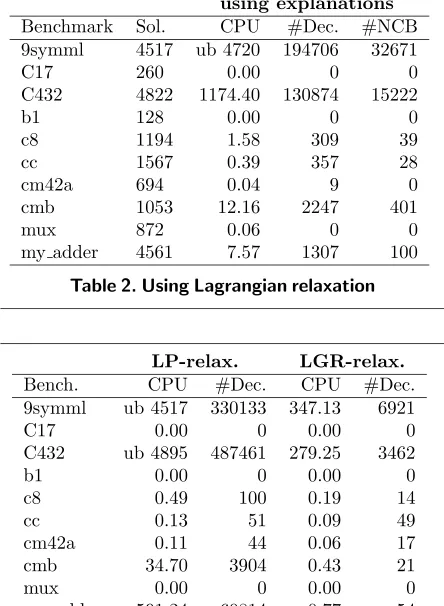
my adder 4561 7.57 1307 100 Table 2. Using Lagrangian relaxation

LP-relax. LGR-relax.

Bench. CPU #Dec. CPU #Dec.

9symml ub 4517 330133 347.13 6921

C17 0.00 0 0.00 0

C432 ub 4895 487461 279.25 3462

b1 0.00 0 0.00 0

c8 0.49 100 0.19 14

cc 0.13 51 0.09 49

cm42a 0.11 44 0.06 17

cmb 34.70 3904 0.43 21

mux 0.00 0 0.00 0

my adder 591.24 60814 0.77 54 Table 3. Heuristic proposed in section 5

In Tables 1 and 2 we present our results for our pseudo-boolean solver using VSIDS heuristic and La-grangian relaxation as the lower bound method. In this table we provide the CPU time in seconds, the num-ber of decisions and the numnum-ber of non-chronological backtracks observed during the search, and evaluate the use of explanations described in section 4.3 when bound conflicts occur. Notice that there is a significant reduction of the search space and time spent in solv-ing these instances.

In Table 3 we can see the results for this bench-mark set when using the heuristic proposed in section 5. Linear-programming relaxation provides good results, but Lagrangian relaxation is able to solve all instances with dramatically better CPU times.

In comparison with the SAT-based linear search al-gorithms [2, 3, 4, 7], our approach is able to perform much better due to the lower bounding procedures in-corporated in our algorithm. All other algorithms find it very difficult to deal with the information from the cost function and are able to solve just the more easy problem instances, as we can see in table 4. In most

in-PBS galena bsolo

Benchmark Sol. CPU CPU CPU

9symml 4517 ub 6453 ub 6986 347.13

C17 260 0.00 0.01 0.00

C432 4822 ub 6577 ub 8070 279.25

b1 128 0.00 0.00 0.00

c8 1194 ub 1542 ub 1528 0.19 cc 1567 ub 1692 ub 1786 0.09 cm42a 694 ub 754 ub 696 0.06 cmb 1053 ub 1490 ub 1476 0.43 mux 872 ub 1321 ub 1333 0.00 my adder 4561 ub 6271 ub 5548 0.77 Table 4. Comparison with SAT-based algorithms

PBS galena1 galena2

Benchmark Sol. CPU CPU CPU

grout-4.3.1 62 ub 64 ub 62 2.85 grout-4.3.2 64 ub 66 594.37 19.42 grout-4.3.3 62 ub 66 ub 62 4.11 grout-4.3.4 60 ub 62 ub 60 6.51 grout-4.3.5 60 ub 64 1373.29 6.02 grout-4.3.6 66 617.61 58.93 8.26 grout-4.3.7 64 1334.94 50.23 0.86 grout-4.3.8 36 ub 44 ub 42 17.90 grout-4.3.9 68 1227.29 150.03 2.24 grout-4.3.10 70 36.16 41.09 0.36

Table 5. Comparison in routing benchmarks

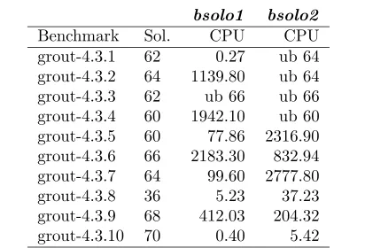
stancesgalena[4] was unable to finish due to memory constraints after several minutes running whilePBS[2] was unable to solve these instances due to time limits. Finally, we present the results for the routing bench-marks.galena1means that the selected learning scheme was the generation of a propositional clause (likePBS andbsolo) while ingalena2the selected learning scheme was the generation of a cardinality constraint (default option of the solver). We also present two columns regarding bsolo. In bsolo1 linear-programming relax-ations are used while inbsolo2we used Lagrangian re-laxations.

bsolo1 bsolo2 Benchmark Sol. CPU CPU grout-4.3.1 62 0.27 ub 64 grout-4.3.2 64 1139.80 ub 64 grout-4.3.3 62 ub 66 ub 66 grout-4.3.4 60 1942.10 ub 60 grout-4.3.5 60 77.86 2316.90 grout-4.3.6 66 2183.30 832.94 grout-4.3.7 64 99.60 2777.80 grout-4.3.8 36 5.23 37.23 grout-4.3.9 68 412.03 204.32 grout-4.3.10 70 0.40 5.42 Table 6. Comparison in routing benchmarks

this benchmark set. These results motivate inte-grating cardinality constraints learning in bsolo and the development of techniques for fine-tuning La-grangian relaxation lower bounding, and for dynam-ically switching between the two lower bound tech-niques.

7. Conclusions

The paper proposes the integration of lower bound estimation procedures with SAT-based techniques for linear pseudo-boolean optimization. We focus mainly in two lower bound methods: linear-programming re-laxation and Lagrangian rere-laxation. We describe a pro-cedure to enable non-chronological backtracking in the search tree when bound conflicts occur. In addition, we also propose the use of information from the lower bound procedure in order to have a more informed heuristic for decision assignment without overhead in the process.

Preliminary results show that for specific classes of instances the integration of lower bound estimation procedures offer a dramatic improvement with respect to linear pseudo-boolean solvers. Results also show that linear search SAT-based algorithms find it very difficult to solve instances when the range of the cost value of feasible solutions is large. When that occurs, the algo-rithm needs a lower bound estimation procedure that provides a tight bound.

Future research work will include improvements on the integration of the lower bound estimation proce-dures as well as the development of different conflict-based learning schemes and improve on the implemen-tation of the data structures.

References

[1] F. Aloul, A. Ramani, I. Markov, and K. Sakallah. Generic ILP versus specialized 0-1 ILP: An update. InIEEE/ACM International Conference on Computer Aided Design, pages pp. 450–457, November 2002. [2] F. Aloul, A. Ramani, I. Markov, and K. Sakallah. PBS:

A Backtrack-Search Pseudo-Boolean Solver. In Sym-posium on the Theory and Applications of Satisfiability Testing (SAT), pages pp. 346–353, 2002.

[3] P. Barth. A Davis-Putnam Enumeration Algorithm for Linear Pseudo-Boolean Optimization. Technical Report MPI-I-95-2-003, Max Plank Institute for Computer Sci-ence, 1995.

[4] D. Chai and A. Kuehlmann. A Fast Pseudo-Boolean Constraint Solver. InDesign Automation Conference, 2003.

[5] O. Coudert. On Solving Covering Problems. In Proceed-ings of the ACM/IEEE Design Automation Conference, pages 197–202, June 1996.

[6] O. Coudert and J. C. Madre. New Ideas for Solving Cov-ering Problems. InProceedings of the ACM/IEEE De-sign Automation Conference, June 1995.

[7] H. Dixon and M. Ginsberg. Inference Methods for a Pseudo-Boolean Satisfiability Solver. InNational Con-ference on Artificial Intelligence, 2002.

[8] J. Hooker. Logic-Based Methods for Optimization. In . Jon Wiley & Sons, 1996.

[9] S. Liao and S. Devadas. Solving Covering Problems Us-ing LPR-Based Lower Bounds. InProceedings of the ACM/IEEE Design Automation Conference, pages 117– 120, 1997.

[10] J. J. J. M. S. Bazaraa and H. D. Sherali. Linear Pro-gramming and Network Flows. 2nd Ed., John Wiley & Sons, 1989.

[11] V. Manquinho and J. Marques-Silva. Search pruning techniques in sat-based branch-and-bound algorithms for the binate covering problem.IEEE Transactions on Computer-Aided Design, 2002.

[12] M. Moskewicz, C. Madigan, Y. Zhao, L. Zhang, and S. Malik. Chaff: Engineering an Efficient SAT Solver. InDesign Automation Conference, June 2001.

[13] G. L. Nemhauser and L. A. Wolsey.Integer and Combi-natorial Optimization. John Wiley & Sons, 1988. [14] T. M. R. Ahuja and J. Orlin.Network Flows: Theory,

Al-gorithms, and Applications. Pearson Education, 1993. [15] A. S. S. Nash. Linear and Nonlinear Programming. In .

McGraw-Hill, 1996.

[16] M. Savelsbergh. Preprocessing and probing for mixed in-teger programming problems. ORSA Journal on Com-puting, 6:445–454, 1994.

[17] T. Villa, T. Kam, R. K. Brayton, and A. L. Sangiovanni-Vincentelli. Explicit and Implicit Algorithms for Binate Covering Problems. IEEE Transactions on Computer Aided Design, vol. 16(7):677–691, July 1997.