Adaptive distance sampling

(1)

ADAPTIVE DISTANCE SAMPLING

John Pollard

A Thesis Submitted for the Degree of PhD

at the

University of St Andrews

2002

Full metadata for this item is available in

St Andrews Research Repository

at:

http://research-repository.st-andrews.ac.uk/

Please use this identifier to cite or link to this item:

http://hdl.handle.net/10023/15176

(2)

Adaptive distance sampling

John Pollard

o n o

Thesis submitted for the degree of

DOCTOR OF PHILOSPHY

In the School of Mathematics and Statistics,

UNIVERSITY OF ST ANDREWS.

(3)

ProQuest Number: 10166155

INFORMATION TO ALL USERS

The quality of this reproduction is dependent upon the quality of the copy submitted.

In the unlikely event that the author did not send a com plete manuscript and there are missing pages, these will be noted. Also, if material had to be removed,

a note will indicate the deletion.

uest

ProQuest 10166155

Published by ProQuest LLO (2017). Copyright of the Dissertation is held by the Author.

This work is protected against unauthorized copying under Title 17, United States C ode Microform Edition © ProQuest LLO.

ProQuest LLO.

789 East Eisenhower Parkway P.Q. Box 1346

(4)

(5)

1. I, John Pollard, hereby certify that this thesis, which is approximately 55,000 words in length, has been written by me, that it is the record of work caiiied out by me and that it has not been submitted in any previous applications for a higher degree.

date signature of candidate

2. I was admitted as a reseai'ch student in April 1995 and as a candidate for the degree of PhD in September 1996; the higher study for which this is a record was carried out in the University of St Andrews bet^teçn 1 9 ^ and 2002.

date signature of candidate...

I hereby certify that the candidate has fulfilled the conditions of the Resolution and Regulations appropriate for the degree of PhD in the University of St Andrews and that the candidate is qualified to submit this thesis in application for that degree.

date

P. h

signature of supervisor

4. In submitting this thesis to the University of St Andrews I understand that I am giving permission for it to be made available for use in accordance with the regulations of the University library for the time being in force, subject to any copyright vested in the work not being affected thereby. I also understand that the title and abstract will be published, and that a copy of the work may be made and supplied to any bona fide library or research, worker.

(6)

Abstract

We investigate mechanisms to improve efficiency for line and point transect surveys of clustered populations by combining the distance methods with adaptive sampling. In adaptive sampling, survey effort is increased when areas of high animal density are located, thereby increasing the number of observations.

We begin by building on existing adaptive sampling techniques, to create both point and line transect adaptive estimators, these aie then extended to allow the inclusion of covariates in the detection function estimator. However, the methods are limited, as the total effort required cannot be forecast at the start of a survey, and so a new fixed total effort adaptive approach is developed. A key difference in the new method is that it does not require the calculation of the inclusion probabilities typically used by existing adaptive estimators. The fixed effort method is primarily aimed at line transect sampling, but point transect derivations aie also provided.

We evaluate the new methodology by computer simulation, and report on suiweys of harbour poipoise in the Gulf of Maine, in which the approach was compaied with conventional line transect sampling. Line transect simulation results for a clustered population showed up to a 6% improvement in the adaptive density variance estimate over the conventional, whilst when there was no clustering the adaptive estimate was 1% less efficient than the conventional. For the haibour poipoise survey, the adaptive density estimate cvs showed improvements of 8% for individual porpoise density and 14% for school density over the conventional estimates.

(7)

Acknowledgements

First I must thank Liz, my wife, for her support, encouragement and understanding over the last 7 yeai's, without her help I could not have done this. Also my two childien Oliver and Anna for their patience while I researched this thesis.

Steve Buckland my supervisor, for his support, guidance and insight throughout this work, and his belief that I could complete a PhD through part-time study.

Phil Hammond my second supervisor, for his advice and willingness to proof read.

To the people of Northwest Fisheries Science Center, Woods Hole, especially Debi Palka, for their work on the experimental harbour poipoise survey, and the crew and observers of the Abel-J who carried out the survey.

(8)

Chapter 1 Introduction

Wildlife abundance estimation is becoming increasingly important as the habitats and reserves of many species are diminished. At the same time the resources to assess these populations are typically limited and so it is desirable to maximise the effectiveness of any surveys peifoimed.

Many wildlife populations occur in loose spatial clusters or aggregations and if the number of aggregations is small, then sample size may be inadequate for reliable estimation, and precision may be poor. With spatially clustered populations, it is therefore attractive to focus potentially expensive surveying resource on the spatial clusters, by increasing sampling in aieas of higher detection. Hence in recent years adaptive sampling has been promoted as a method suited to clustered populations. Adaptive sampling adds surveying effort when the survey adapts and thus, unlike many basic sampling estimators, the analysis methods do not assume the survey effort is randomly allocated.

Distance sampling (see for example, Buckland et ah 2001, Buckland et ah 2002, Burnham et ah 1980, Thomas et ah 2002) is widely used to estimate animal abundance, particularly in the form of line and point transect sampling. Line and point transects do not require all animals within a sampled aiea to be detected, but instead model the probability of detection, based on the distance of the detected animals from the observer. This modelled detection junction is then used to scale the number of observations to account for the animals that were not detected.

(12)

Seber, 1992) who have done much to develop this area over the last fifteen or so years.

Whilst the initial premise is to improve estimator precision a new density estimator is developed which can also optimise survey coverage, allowing a survey to complete within a fixed total sampling effort. It does this through the efficient allocation of surveying resources and is able to compensate for lost surveying time due to bad weather or other external factors. Although precision improvements can be achieved, this is highly dependent on the underlying spatial clustering of the population, and the true benefit of the methods is likely to be the improved coverage.

1.1 Thesis Outline

Chapter 1 provides a brief overview of the adaptive cluster sampling methods of Thompson, Seber and Ramsey and also of distance sampling. Hereafter, rather than reference all three names we typically refer to just Thompson, for example, Thompson’s methods. For brevity, we also refer to the methods as adaptive sampling or adaptive methods, and omit the complete adaptive cluster sampling title. It is expected that readers will be more familiar with distance sampling than Thompson’s methods, and so the adaptive sampling is also illustrated with a brief example. We complete the chapter by introducing Thompson’s basic adaptive estimators used to build the estimators of Chapters 2 and 3.

In Chapter 2 we begin by combining Thompson’s adaptive methods with point transect sampling, and refer to this simply as adaptive point transect sampling. Four basic estimators ai*e developed and then the methods are extended to allow the inclusion of covariates in the detection function estimation, following the approaches of Marques (2001) and Borchers (1996). A basic simulation is perfoimed and the pros and cons of various patterns for the additional adaptive point transects explored. We close the chapter with a general discussion which also considers how the methods may be applied in the field.

(13)

follows a similar foimat to Chapter 2, but concentrates on the changes required for line transects. With Thompson’s methods, the total surveying effort is unknown at the start of the survey. Thus we also discuss approaches for keeping the total effort within reasonable limits.

In response to the unknown total survey effort. Chapter 4 develops a new estimator, where the survey can be completed using a fixed total effort, teimed the PB method. First a line transect estimator is developed and tested through simulations. As with the Thompson-based adaptive point and line transect estimators, the approach is extended to allow the inclusion of covaiiates in the detection function estimator. A point transect estimator is also derived. Much of this chapter is drawn from Pollard and Buckland (1997) and Pollai'd, Palka and Buckland (in press).

Chapter 5 applies the new fixed total effort estimator to an experimental harbour porpoise line transect survey. The experiment compares adaptive and conventional surveys run over the same transects in similai’ conditions. We explain how the survey configuration was chosen, consider the field procedures, discuss the analysis and review the results. The analysis and results of this survey were originally reported in Palka and Pollard (1999).

We close with a discussion compaiing the vaiious methods and review both the benefits and drawbacks of the adaptive procedures developed. We also consider the combination of conventional and adaptive survey methods, so that conventional estimates can be still be extracted and thus allow compaiison with previous survey results.

(14)

1.1.1 Conventions

Some of the terminology used can have alternative meanings, particularly between the two approaches of adaptive and distance sampling. In this section we clarify a number of the teims to avoid confusion.

The thesis considers wildlife abundance, and thus the items in the populations sampled are typically refeiTed to as animals. However the methods aie not restricted to these alone.

Thompson’s methods refer to the combined adaptive cluster sampling developments of Thompson, Seber and Ramsey, and adaptive sampling or Thompson’s adaptive methods is used in place of adaptive cluster sampling. Thompson developed four core estimators for adaptive sampling (see section 1.3.1) and these aie called the Thompson-based estimators, or the basic adaptive estimators. Thompson uses a condition which, if met, triggers adaptive sampling behaviour. This is often called the trigger condition, adaptive trigger or just trigger.

Within the context of this thesis, distance sampling refers to either line or point transect sampling, or some variation on these such as trapping webs. Standard distance sampling is named conventional, as in conventional line transect sampling or conventional point transect sampling.

(15)

The survey region is the area of interest for which abundance is being estimated, and the population the animals contained within it. Thompson’s methods overlay the survey region with a grid of sampling units, which we also refer to as grid units or units. When the method selects a unit for sampling, then depending on the type of survey either a line transect or point transect sample is perfoimed within the unit. We refer to the line transect sampling strip and the point transect sampling plot or plot, as the ai'eas sampled from the lines or points up to some truncation distance. The surveyed area represents the total area of all sampling strips or plots for every unit in the grid, whether sampled or not. This may be more or less than the area of the survey region, depending on whether sampling strips/plots in adjoining units overlap. To accommodate this, when producing estimates for the survey region, the estimates relating to the surveyed area have to be adjusted according to ratio of its area to the survey region aiea.

Where possible, notation is maintained in accord with both distance sampling and Thompson’s methods. However this has not always been possible, due to the number of paiameters in use, and there have been some clashes. In such cases, if feasible, context is maintained by using a similai' letter from an alternative alphabet or at least a letter that represents the paiameter. Thus for example in the adaptive point transect chapter, w was already used in a number of the Thompson estimators and so the truncation radius is represented by R, whilst in the adaptive line transect chapter the truncation half-width is represented by W.

1.2 Overview of Distance Sampling

(16)

requirement to detect all objects. Instead the observer records the distance to each observation, and the sample distances aie used to model the probability of detecting an object based on its distance from the line or point, refened to as the detection function. The detection function along with the sample size can then be used to

estimate the actual number of animals in the sampled strip or circle, which is then used to provide an overall estimate of abundance in the survey region. The basic estimators assume: that all animals are detected on the line or point; that the probability of detecting an object decreases as the distance from the observer increases; that the distances to the objects aie accurately recorded; that objects aie detected at their initial position and there is no movement in response to the observer; and that the lines or points have been placed randomly with respect to the distribution of objects. Approaches are available to relax these assumptions but for this introduction we concentrate on the basic methods.

Free softwaie is available for the analysis of conventional distance sampling (Thomas et aL, 2002; Laake et al, 1996) and a comprehensive introduction to the methods and their application is provided by Buckland et al. (2001).

1.2.1 Line Transect Sampling

In line transect sampling a number of randomly placed lines are traversed by the observer, and the perpendiculai* distances to all objects observed are recorded. In some cases the observer may instead record the radial distance to the object and the angle between the sight line and the trackline being followed, which is then easily converted to a perpendiculai* distance using basic trigonometry. Let the total length of transect surveyed be L, the number of objects observed n, and the detection function g(jc), where x is the distance from the line.

(17)

D = É à 2jXL

If each observation is of a group rather than an individual animal, then the density of individual animals is given by

A . .

where

Ê(s) is an estimate of the expected mean group size in the population

1.2.2 Point Transect Sampling

In point transect sampling, the observer is located at a point and records the radial distances to observations. In this case let the total number of points sampled be k, the total number of objects observed n, and the detection function g(r), where r is the radial distance from the point to an object. For point transects we want to estimate the effective radius p, which is the radius of a circle such that if all objects were detected from each of k points, we would expect to detect E(n) observations. Thus the effective area for a point is and the total effective area across all the sampled points is kizp^. An estimate of the object density is given by

D

knp'^

If the observations relate to groups of animals, then the density estimate can be converted to a density of animals by multiplying by an estimate of the expected mean group size.

(18)

1.3 Overview of Adaptive Cluster

Sampling

To give an insight into Thompson’s methods, we provide a brief overview of adaptive cluster sampling, hereafter referred to as adaptive sampling. The approach is aimed at the sampling of rare, but spatially clustered populations, and works by sampling additional units, above the initial sample, when the variable of interest for a sampled unit meets some trigger condition. In our case, this is typically when the count of animals exceeds some preset limit.

The basic adaptive process for Thompson’s methods operates as follows. A number of initial units are selected at random and sampled. If the number of observations in a sampled unit satisfies some condition (also teimed here the trigger condition, or trigger), then units in the neighbourhood of the triggering unit are also sampled. The neighbourhood defines a symmetric pattern of units and its layout is pait of the survey design. If any of the adaptive units in the neighbourhood meet the condition, then the neighbourhood of each of these units is also sampled. The process repeats until no newly sampled units meet the condition.

The combination of an initial unit and its associated adaptive units is termed a cluster. Within the cluster, any units which do not meet the condition are termed edge units, whilst any units which meet the condition foim a network. Any initial unit that does not meet the condition is also a network, consisting of a single unit. The neighbourhood can be defined as any pattern suiTounding the sampled unit, and may not be contiguous. However it must have the property that the sampling of any unit within a network will then also sample all other units within the same network.

The final sample will therefore consist of a network for each of the initially sampled units. However it is possible that the networks from two or more separate initial units may merge into one larger network.

(19)

randomly selected (Figure 1.1). If a unit is sampled then all animals within that unit are detected.

[image:19.612.13.537.21.599.2]

4—-t—-Initial Units

Figure 1.1: A grid of sampling units is overlaid on the survey region. Initial sampling units have been selected and are shown as shaded (yellow). Animals in the population are shown as black dots.

In this example the trigger condition is defined as one or more observations in a sampling unit, and adaptive units are added on the four adjoining edges, above, below and to the left and right, of any unit that meets the condition. Two initial units meet the condition and so adaptive units are added to these units (Figure 1.2).

Adaptive Units

Figure 1.2: Adaptive units are added in the four adjacent units above, below and to the left and right of any initial units that meet the trigger condition of one or more observations. Adaptive units are shown with (blue) cross-hatching.

(20)

1 1 ^ ' "_{_}₁ _{i l l , ,}

' ₁ _{• 1 i 1 ; 1}

; : ' ■ I

- J I t 1

“ 1 1

; i

1 !

1 r n

L l i l J

i ! ■

3 1 * 1 ,

i i i ■

■ ■ 1

• ! 1 i ; .

r ! ; -

1 “ —

1 ! _{■ i ‘ i _}

. I « _1 ‘ ‘ t »

1 1 1 ; 1 i : i !

i — —Clusters

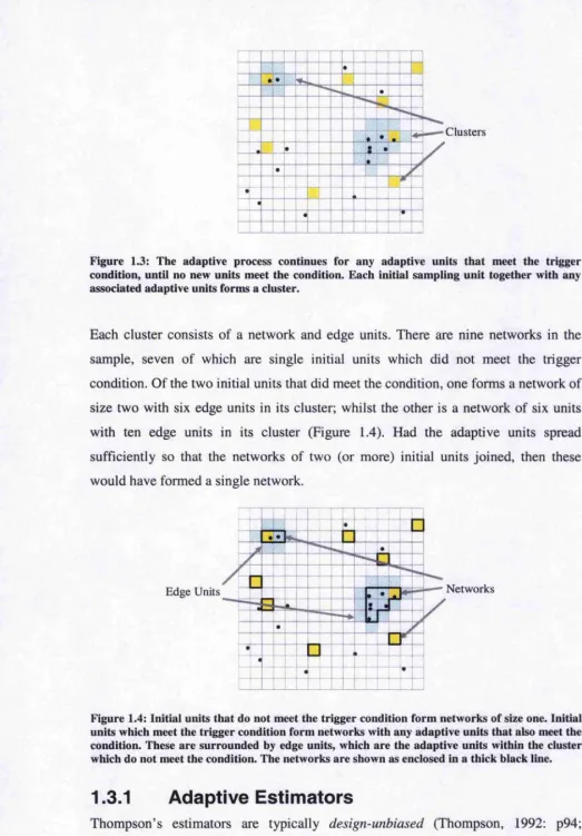
Figure 1.3: The adaptive process continues for any adaptive units that meet the trigger condition, until no new units meet the condition. Each initial sampling unit together with any associated adaptive units forms a cluster.

Each cluster consists of a network and edge units. There are nine networks in the sample, seven of which are single initial units which did not meet the trigger condition. Of the two initial units that did meet the condition, one forms a network of size two with six edge units in its cluster; whilst the other is a network of six units with ten edge units in its cluster (Figure 1.4). Had the adaptive units spread sufficiently so that the networks of two (or more) initial units joined, then these would have formed a single network.

Networks

Edge Units _-4

Figure 1.4: Initial units that do not meet the trigger condition form networks of size one. Initial units which meet the trigger condition form networks with any adaptive units that also meet the condition. These are surrounded by edge units, which are the adaptive units within the cluster which do not meet the condition. The networks are shown as enclosed in a thick black line.

1.3.1 Adaptive Estimators

[image:20.612.16.540.21.772.2]

(21)

of the variable of interest, for example the count of animals in each quadrat, are considered fixed and the selection probabilities introduced by the design are used to estimate the abundance and associated variance, etc. Thus a design-unbiased estimator is unbiased whatever the underlying population.

The Thompson-based estimators are derived from the unequal probability sampling estimators of Hansen-Hurwitz (Hansen and Hurwitz, 1943) and Horvitz-Thompson (Horvitz and Thompson, 1952). We now describe these two estimators with respect to a simple random sample of units (quadrats) from a sui'vey region with the variable of interest being the count of animals made in each unit sampled.

The Hansen-Hurwitz is an unbiased estimator for sampling with replacement. It considers the draw-by-draw selection probabilities for each unit in the sample and these probabilities are used to weight the sample size for that unit in the sample, so that the sum of these weighted values provides an estimator of the population total. If a unit is drawn twice, then its count is used twice in the summation. The Hansen- Hurwitz estimator for the population total and its variance are

1 T / / Æ \ _ L

HH

■iti

y where

k is the number of units in the sample y, is count of interest in for the i‘'^ unit

p, is the probability of selecting the i‘^^ unit in a draw

The Horvitz-Thompson estimator considers the probability of including any unit in the sample. It only uses the distinct units in the sample, so that if a unit is drawn multiple times it is only used once in the estimator. The Horvitz-Thompson estimator is unbiased for sampling both with and without replacement. Its estimate of the population total and its vaiiance aie:

and = _n,

1=1 (=1

where

is the number of distinct units in the sample

(22)

y,. is value of interest for the i‘*^ unit

7t^ is the probability of including the i^^ unit in the sample is the probability of including both the i^^ and units in the sample

Rather than considering the count of animals in each quadrat, Thompson’s adaptive estimators use the count of animals in each network and consider the probability of the networks being included. When the trigger condition is a single detection, there are no animals detected in edge units, however if the trigger condition is greater than one, then the count of animals in any edge units are not included in the sample when producing estimates.

We complete the introduction by outlining the basic adaptive sampling estimators for Thompson’s methods. We consider two categories of adaptive sampling design and for each design Thompson has both a Hansen-Hurwitz and a Horvitz-Thompson- based estimator, making a total of four basic estimators.

The two survey designs are a Random Initial Sample (RIS) and a Systematic Initial Sample (SIS). As the name infers, a RIS design survey has the initial units selected at random, and adaptive units are added to any initial units which meet the trigger condition. The RIS design estimators for this are described further in Thompson (1990). A SIS design consists of primary units and secondary units. The secondary units are systematically aiTanged to form the primary units. The primary units are however still randomly selected. In this case adaptive units are added to any secondary units that meet the trigger condition. More detailed descriptions of the SIS design estimators are found in Thompson (1991). In Chapters 2 and 3 the two designs are explained in more detail with specific reference to point and line transect surveys.

(23)

RIS Design Estimators

RIS Design: Hansen-Hurwitz-based Estimator

Thompson developed an estimator from the Hansen-Hurwitz estimator for sampling with and without replacement (Thompson, 1992: p271). The estimate of the mean number of objects per unit is

(11)

where

jevfi

k is the number of units in the initial sample

jj is the y value (value of interest) for the j^*^ unit in network y/^ \}f . is the network which includes the i*^^ initial unit

nii is the number of units in network y/.

and the conesponding variance estimator, assuming the initial sample is selected without replacement, is

where

K is the total number of units in the survey region

RIS Design: Horvltz-Thompson-based Estimator

Thompson has also developed an estimator from the Horvitz-Thompson estimator for sampling with or without replacement (Thompson, 1992: p273). The without replacement estimator of the mean number of objects per unit is

* 4 #

<■»

where

Uf =1

V is the number of distinct networks in the sample k is the number of units in the initial sample

(24)

yi Oi K ti

is the sum of the y values (value of interest) for the i‘^^ network is the probability that the i^^ network is included in the sample is the total number of units in the survey region

is the number of units in the i^* network.

and the conesponding variance estimator is

where

= 1- ' +

1/

'K '

1/

4 /

(1.4)

SIS Design Estimators

SIS Design: Hansen-Hurwitz-based Estimator

From Thompson (1992: p293), for a systematic or strip adaptive survey, an estimate of the mean number of objects per unit is given by

1

f h=\ where

(1.5)

1=1

r M

A/, 3^/

is the number of primary units in the sample

is the number of secondary units in each primary unit is the number of networks that intersect the h^*^ primary unit is the sum of the y values (value of interest) in the i‘^ network is the number of primary units that intersect the i^'^ network

An unbiased estimate of the variance is given by

varL«3] = ^

r 1- —

R (1.6)

where

s i =

_-A)

•1- /i=l

(25)

This is based on the initial intersection probabilities and is related to the Hansen- Hurwitz estimator.

SIS Design: Horvitz-Thompson-based Estimator

From Thompson (1992: p295), for a systematic or stiip adaptive survey, an estimate of the mean number of objects per unit is given by

1 _(1.7)

where

R “ r =1

I '

M is the number of secondary units in each primary unit R is the number of primary units in the survey region

yt is the sum of the y values (value of interest) in the i^^ network ai is the probability the i“' network is included in the sample ti is the number of primary units that intersect the i^^ network r is the number of primary units in the sample

V is the number of distinct networks in the sample

The corresponding variance estimator is

where

and Uh

R — t;

+^ R - t ^

(1.8)

(26)

Chapter 2 Adaptive Point Transect Sampling

2.1 Introduction

This chapter explores the application of Thompson’s adaptive methods (see, for example, Thompson, 1992; Thompson and Seber, 1996) to point transect surveys.

Point transect sampling (Buckland et ah, 2001), also known as variable circular plots, is most commonly used in ornithology. Extensions to the method include trapping webs (Anderson et al., 1983; Buckland et al., 2001; Parmenter et al., 2002) and cue counting (Hiby, 1982; Hiby, 1985; Hiby and Hammond, 1985; Buckland et al, 2001).

The typical approach is to define a series of points in the survey region. These points can be located either randomly; on lines located randomly or systematically; or on a grid randomly located on the area. At each point the observer records the distance to any animals seen there. All animals close to the point must be detected whilst as the distance increases it is expected that the proportion of animals detected will decrease. The detection distances are used to estimate the detection function, which is in turn used to estimate the effective area. That is the area of a circle at which, assuming all animals to be detected, would produce the same count of detections as was actually recorded. Alternatively this can be considered as the area of a circle such that as many animals are seen outside this circle as are missed inside it. Assuming single animals for each observation, the density estimate is then simply given by the mean number of observations per point divided by the effective area.

(27)

line so it is more suited to surveying patchy habitats and the observer can take the most direct or easiest route to and from each point. In addition markers can be positioned at set distances, making the observer’s task easier, and only the distance and not the angle is required to be estimated by the observer.

A point transect survey typically has at least 20 points, but there may need to be more to get sufficient observations for reliable estimation of the detection function. For raie species this may require hundreds of points. To provide acceptable levels of precision the survey should aim for a minimum of around 75-100 detections of the prime species being surveyed (Buckland et ah, 2001: p240).

Within this chapter we combine adaptive with point transect sampling by treating each point as a sampling unit. Thompson’s adaptive estimates are used to obtain estimates of the mean number of detections per unit and the expected group size whilst sightings data are pooled across all sightings to improve estimation of the detection function. We start by developing combined adaptive and point transect sampling estimators for two basic survey designs; a random and a systematic initial sample. These teims aie explained in the following section, Survey Designs. For each design both a Hansen-Hurwitz and a Horvitz-Thompson-based estimator aie developed, making a total of four basic estimators. Many surveys will use systematically positioned initial points, however it is widely accepted that if the grid is randomly located on the survey region then the points can be considered random. Thus later in the chapter we focus on a Horvitz-Thompson-based estimator with a random initial sample.

The estimators include a number of subscripted variables which can at first appear confusing. For clarity a simple example, with full working, is presented for each of the four basic estimators considered.

(28)

The observers will need to move between points, referred to here as ojf-ejfort, where off-effort encompasses both the time taken and any resource used in the travel (e.g. a vehicle). By the very nature of point transect sampling, the additional points sampled in the adaptive neighbourhoods will introduce an amount of off-effort travel. However for a point transect survey this is likely to be small, when compared to the off-effort travel between the points on a conventional survey. Thus the total off- effort travel for an adaptive survey will potentially be less than that for a conventional point transect survey, with an equivalent number of points surveyed. This is akin to the gain from cluster sampling but in this case the sampled clusters are expected to occur where animals are known to be present.

2.1.1 Survey Designs

In this chapter we consider two types of survey design, one classified as a Random Initial Sample (RIS) and the other as a Systematic Initial Sample (SIS). The terms refer to the selection of the initial survey points; adaptive points are then added according to the adaptive neighbourhood pattern in use. These two terms are not immediately intuitive and warrant further explanation.

;

I -

i

“ i + t

-Î

ti

tii

.lllf'

G a

j t f

! - ( •

! r^ - \ .... . _

—I----Figure 2.1: RIS point transect survey designs, with the sampling points shown as solid (yeilow) circles. In the left hand design points have been selected at random on the grid. The right hand design is a systematic grid of points, and (given a random start location) the points are assumed to he independently located.

[image:28.612.7.540.33.654.2]

(29)

each line is similar to the space between lines, we obtain a systematic grid of points. In distance sampling, if the systematic grid is randomly located, it is commonplace to consider the points as random and hence this is considered a RIS design, with the result that variance is slightly overestimated. If the interline spacing is significantly different from the point spacing on lines, it should be treated as a systematic sample and thus a SIS design. Examples of RIS designs are shown in Figure 2.1 and SIS designs in Figure 2.2.

D

u i

_{I ■ i.}

be

M

b e

I ! !

[image:29.612.16.545.26.792.2]

-r :

Figure 2.2: SIS point transect survey designs, with the sampling points shown as solid (yellow) circles. In the left hand design, points are systematically located in lines (the primary units), which are then systematically distributed over the survey region. In the right hand design points are also systematically distributed in lines, which in this case are then randomly (in the horizontal plane) located on the survey region.

2.2 Theory

In this section we develop the adaptive point transect estimators. Point transect sampling is commonly used for songbirds where animals are typically recorded as individuals. However throughout this chapter we follow a generic approach and allow for observations to be a single or multiple animals. Should animals be recorded as individuals then the number of animals per observation is set to 1 and all estimators will function correctly.

2.2.1 Point Transect Sampling Basic Formulae

From Buckland et al (2001: p55) the density of a population from point transect sampling is given by

(30)

E(n) is the expected number of animal groups in the sample h(0) is the derivative of the probability density function/(r)

evaluated at r=0

E(s) is the expected group size for the population k is the number of points

Replacing parameters by their estimators, an estimate of the density is given by

(2.1)

Using the delta method (Seber, 1982: p5-7) the variance can be estimated by

vâi*[n] vâr[ë(o)] vâr[ê(j)]_{---4 r} _{TZ H ^...} vâr(ô)- •

k o ) f .

(2.2)

2.2.2 Merging Adaptive and Point Transect

Sampling

Defining the survey region as the aiea of interest and the population as animals contained within it, the basic approach is to overlay the survey region with a grid of units. Units are then selected according to some sampling algorithm and within each of these units a point transect survey is conducted. For each point sampled the surveyed circle, up to the truncation radius, is refened to as the plot, with the centre of the plot centred within the grid unit. The shape of the units and the truncation radius of the point transect are discussed in section 2.3, Grid Design; however initially it is probably easiest to visualise the units as squaies, as shown in Figure 2.1 and Figure 2.2.

(31)

Thompson’s methods are used to get unbiased estimates for the key parameters of the expected number of observations (groups detected, where a group may be a single or multiple animals), and the expected group size. However we pool observations across all points to produce an h{o) estimate. This assumes no heterogeneity is introduced from the adaptive process and we initially assume that the probability of detection on the point, go, is 1. The estimates are then fed into the point transect equations to provide a density estimate.

000

[image:31.612.10.536.18.765.2]

Plots smaller than units _{Plots larger than units}

Figure 2.3: Point transect plots may be larger or smaller than the units they are located within. Thus the surveyed area is given by the total number of plots, K , in the survey region, multiplied by the area of each plot. Point transect plots are shown in yellow, on a grid of square units.

It should be noted that in conventional distance sampling density estimates, we use n as the number of observations in the sample. Here we use Thompson’s methods to estimate n , the mean number of observations per point, and â, the mean number of individual animals detected per point. Note that in general an observation is a group of animals: a > n . We also use N to represent all animals in the survey region and Ng as the number of animal groups in the survey region.

Thus

N = f^ . x=\ where

is the number of animals in the observation

(32)

number of individual animals (detected and undetected) in the sui^veyed area. The surveyed area is a notional area and, as already stated, may be larger or smaller than the actual survey region. Thus the total number of animal groups in the survey region is obtained by appropriate scaling of t;

jV _ Survey Region Area _ ^ Surveyed Area

Similarly, the total number of animals in the survey region is given by

A f = Survey Region Area ^ (2.4)

Surveyed Ai*ea

Imperfect Detectability

Thompson’s methods are typically founded on all animals being observed within a unit, whilst the underlying premise of distance sampling is that only a proportion of animals aie observed. Thompson and Seber (1996: Chapter 9) provide approaches to deal with this, based on dividing the population estimate by the probability of detection, as is done with distance sampling. We show here that this means the underlying Thompson based adaptive estimators for the count of objects and animals remain unchanged.

From a distance sampling perspective the probability of detection is estimated and for many practical applications this can be assumed to be the same for each object in the population. So, initially, we assume the probability of detection is equal for all objects, and this is included via the pooled

/i(o)

estimate.

For an estimated equal probability of detection for all objects, Thompson and Seber (1996: p219) simply assume that the expected number of objects detected, E{xo), in the surveyed aiea, is given by the number of objects in the surveyed area, t, multiplied by the probability of detection, p. So that

£(r„) = ^

and thus an estimate of the number of objects in the surveyed area is given by

P

(33)

detection probability. This is analogous to the way the point transect density estimator (see equation 2.1) incorporates an estimate of the probability of detection at the point, using h{o) . This probability of detection is used to scale up the density estimate, accounting for missed animals. The variance is then estimated with components from: the number of observations; the detection function estimate; and the group size estimate.

Thus with an equal probability of detection (at distance x from the point) for all animals the adaptive formulae of Thompson and Seber are directly applied with the distance sampling equations.

However methods are also available to allow for unequal detection probability, so that each animal has a different probability of inclusion in the sample. See, for example, Borchers (1996), Marques (2001) and Strindberg (2001). Later in the chapter this type of approach is used to expand the framework and allow each animal to have a unique probability of detection. This can also be used to relax the requirement for all objects to be detected on the point, which would in the past have been managed by incorporating an estimate of go into the divisor of the density estimate (e.g. Bucldand et al, 1993: p57).

Expected Number of Observations

The expected number of observations across the kg points surveyed is E{n). Thus the expected number of observations per point (the expected encounter rate), E(îî) is

given by

E{n) =

^

so that

E{n) = E{n)-k,

and an estimate of the expected mean number of observations in the sample is Ê{n) = ê(n)-k,

Expected Group Size

(34)

Let

a be the total number of animals observed in the sample

aj be the total number of animals observed at the point

ajx be the number of animals in the observation of the point So

~ 2 ^ ^ jx

X = l

where

tij is the number of detections (animal groups) at the point

and

M where

ks is the number of points surveyed

Let £'(a) be the expected total number of animals observed in the sample, had there been no adaptation, and e{ïï) the expected mean number of animals observed per

point. Then

E{a) = E{a)-k,

SO that an estimate of the expected number of animals observed in the sample, is Ê{a) = ê{â)-k,

and an estimate of the expected gi'oup size is given by

A /) g(«) È{â)

Ê{n) Ê{n)-k, ê(n)

Density Estimates

(35)

So substituting Thompson’s estimators for the number of observations and mean group size estimator in the point transect estimators (equations 2.1 and 2.2) gives a density estimate of:

D _ È[n)-h{0)-Ê(s)

Â(0)

ÉW

Æ(râ)-ft(o)'Æ(s)

where È{n)

È{n)

m

È{s) k.K and

I n

is an estimate of the expected number of observations in the sample

is an estimate of the expected mean number of observations per point

is an estimate of the derivative of the probability density function/(r) evaluated at r=0

is an estimate of the expected group size for the population, is the number of points in the survey

var(D)=D2. var[£(«)] ^ var[^(o)] ^ vâr[ê(.y)]

[ Ê { n ) f [% )]' [ê {s) ]

With the group size estimated by the mean observed group size then the estimate simplifies to

^ Ê(n)-h(0)-Ê{s) Ê{n)-h{0)-Ê(a) _ h{0)-Ê{â)

27t 2n ■ Ê{n) 2n

and

ft(0)] , Vâr[g(â)]

(2.5)

vâr(ô)=Ô^- var[/z(U)j var[A(6

_ [% )]' ^ [Ê(â)] (2.6)

The density of animal groups, Dg, is obtained by replacing the group size estimator, Ê{s) by 1 giving

Ê{n)‘h(0)

(36)

v â r (ô J = D /- vai\ . . .r[fi(n)] vâr[ft(0)]+

[ # ) ] '

ko)]'

(2.8)

2.2.3 Assumptions

The basic point transect sampling assumptions apply, although these can be weakened or removed using advanced distance sampling strategies:

(i) Probability of detection on the point is 1, or suitable methods are used to estimate

(ii) There is no size bias (the probability of detection is independent of group size).

(iii) There is no responsive movement of animals in advance of detection.

In addition, we begin with the following additional assumption in place:

(iv) Probability of detection is independent of whether or not effort is adaptive, i.e. probability of detection is only a function of distance from the point and the adaptive procedure does not induce heterogeneity in the h(0) estimate.

Approaches to reduce the need for assumptions (i), (ii) and (iv) are dealt with later in this chapter,

2.2.4 Adaptive Point Transect Sampling with RiS

Design

(37)

RIS Design: Hansen-Hurwitz-based estimators

Taking Thompson’s Hansen-Hurwitz-based estimator, and concentrating on sampling without replacement (equations 1.1 and 1.2), we produce unbiased estimates of the expected mean number of observations per point, ), and the expected mean number of animals observed per point, ).

)

Estimate for RIS Design

Applying equations 1.1 and 1.2 to the point transect surveys gives an estimate of expected mean number of observations per point of

= (2-9)

/C

where

JWi

k is the number of points in the initial sample

\j/i is the network which includes the i‘*^ initial point nii is the number of points in the network

Hij is the number of observations at the point within the network ¥i

The estimate of vaiiance, assuming the initial sample is selected without replacement, is given by

))= ))' (2.10)

where

K is the number of (potential) points in the survey region

) Estimate for RIS Design

Similai'ly an estimate of the expected mean number of animals observed per point is given by:

£(«««) = 7 Z “.- (2.11)

X 1=1

(38)

M. =

m

Z Z «

ijX

UjX is the number of animals in the observation of the point

within the network y/^

The estimate of variance, assuming the initial sample is selected without replacement, is given by

- l \ JL^ I A?

(2.12)

Example 2.1

Consider the example shown in Figure 2.4. This has been simplified to demonstrate the calculations; in reality an initial sample would typically be expected to be significantly larger, of the order of 100 or 200 points. The survey region has been overlaid with a grid of squares, with points centred within each square. Four initial points are randomly selected, without replacement, so ^ = 4, and the grid is 8 by 8 giving K = 64. The trigger condition is the observation of one or more animal. Three of the points meet this condition and so additional points are added; in this case the neighbourhood is defined as the points immediately above, below and to the left and right of the initial point.

[image:38.612.16.539.21.689.2]

6 ')

(39)

[image:39.612.8.543.20.750.2]

Figure 2.5 shows the results of adding neighbouring points to the initial points that meet the trigger condition. Three of the neighbouring points meet the trigger condition and their neighbourhoods are also added.

s /

■ < 1

? S

n _>•■<

1 1

1--- — —

Figure 2.5: Neighbourhood points, shown as shaded circles, have been added to the initial points that meet the trigger condition of at least one observation.

Figure 2.6 shows the completed survey with all additional points added where initial points have met the trigger condition. Two of the initial points both belong to the same network. There are three distinct networks; however one of these appears twice in the analysis by the nature of the Hansen-Hurwitz estimator. Labelling the initial points 1 to 4 working from the top of the survey region to the bottom, and units within a network from 1 to n, working from left to right and top to bottom within a network, the data are summarised in Table 2.1.

\ /

\

J

\ / / N\ y —

/ \

s / _{>'< s /}_{/ \}

/ \

>'■<

r A / s

\

J

— 0 / !

7 \ K

J

(40)

[image:40.612.83.486.77.487.2]

Table 2.1: Summary of data for Example 2.1. Note as the 3*^^ and 4^ Initial points are both part of the same network, they share the same values for «ÿ and

In itia l P o in t nii ttii CliiX

1 m i= l n ii- 0 n/a

2 m 2=l fl21=2 0211=3

0212=1

3 m3=8 n s i- l 0311=2

H32=2 0321-1

0322=1

U33=2 0331=2

0332=2

Îl34=2 0341=1

0342=4

n35=3 0351 =2

0352=1

03532=1

n36—l 0361 =2

1137-1 0371=3

1138=1 0381=1

4 m4=8 1141=1 0411=2

1142=2 0421=1

0422=1

ri43=2 0431—2

0432=2

1%44=2 0-441=1

0442=4

1145=3 0451 =2

0452=1 0453=1

Ïl46=l 046I =2

Il47=l 0471=3

tl48=l 0481=1

Calculation of È{n„fj )

Applying equations 2.9 and 2.10 we get

w, =

(o)=o

So

and

= -(2) = 2

W3 = —(14-2 + 2 + 2 + 3 + 1 + 1 + l) = l .625

W4= i( l + 2 + 2+2+3 + l+ l+ l) = 1.625

8

(41)

64 • 4 • {4 " l) = 0.1868

(0-1.3125)"+(2-1.3125)" +

(1.625-1.3125)" +(1.625-1.3125)'

C

alculation of

Ê(a^„ )

Similarly applying equations 2.11 and 2.12 gives:

H,=i(0) = 0

= —(1 + 3) = 4

«3 = 0(2)+ (1 + 1)+(2 + 2)+(1 + 4)+(2 + 1 + 1)+(2)+(3)+(i)) = 2.875

Wj = —((2)+(1 +1)+ (2 + 2)+ (1 + 4)+ (2+1 + 1)+ (2)+ (3) + (1)) — 2.875

8

So

and

) = ~ (0 + 4 + 2.875 + 2.875) = 2.438

\\ (64-4) f ( 0 -2.4375)"+ (4-2.4375)" +

/ „

64 • 4 • (4 - 1)

I

(2.875 - 2.4375)" + (2.875 - 2.4375)" = 0.6848

RIS Design; Horvitz-Thompson-based estimators

We now use Thompson’s Horvitz-Thompson-based estimator for sampling with or without replacement (equations 1.3 and 1.4), to produce unbiased estimates of expected mean number of observations per point, ê(«^j.), and the expected mean number of animals observed per point, Ê(â^y. ).

e{^ht

) Estimate for RIS Design

Applying equations 1.3 and 1.4 to point transect surveys gives an estimate of the expected mean number of observations per point of

nij

, V Z

”i/-E{n„) = - Y ^ (2.13)

A . i_ i M j.

(42)

a^=l

K

V

mi

Oi

k

'K -m ,''

//

J

is the number of points in the survey region is the number of distinct networks in the sample is the number of points in the i*'^ network.

is the number of observations at the point within the i‘*^ network

is the probability that the i**‘ network is included in the sample is the number of initial points

The vaiiance is estimated by

nil m,,

V

a,a,)

^ 1=1 /;=! with

and

^ii, -1 -

_{. k}

+

'K -m ,'' 'K - nil - Mil

'1

^

// 'K'\

)

I

k

j

k

1/ .0

(2.14)

E{affp)

Estimate for RIS Design

An estimate of the expected mean number of animals observed per point is given by:

where

(%, = 1 -

OijX

(2.15)

'K -m ,''

/

. k y

/

J

is the number of animals observed in the observation of the point in the i*^ network.

(43)

with

and

h : . . . ,—

% = 1 - ( K ~ m u\ (K-~m^~ m,, ^

(2.16)

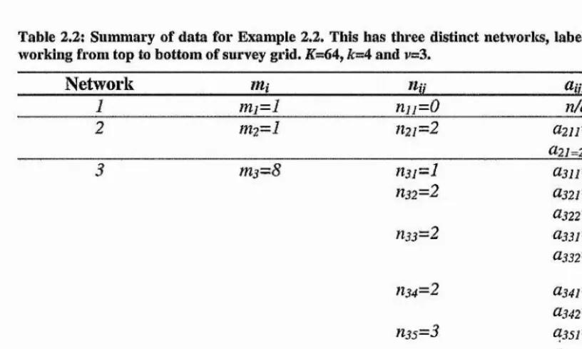
Example 2.2

[image:43.612.81.489.394.638.2]

Using the survey given in example 2.1, but assuming the initial points were selected without replacement, then the survey has 3 distinct networks. Labelling the networks as 1 at the top of the grid, 2 in the middle and 3 at the bottom, the data are summarised in Table 2.2. The total number of units in the suiwey region is K-6A, the number of initial points, k=A and the number of distinct networks, v=3.

Table 2.2; Summary of data for Example 2.2. This has three distinct networlcs, labelled 1 to 3 working from top to bottom of survey grid. Æ=64, /c=4 and v=3.

ni3=8

Network nii na OiiX

1 mi=l nn=0 n/a

2 m2=l 1121=2 0211=3

021=2=1

1131—1 0311=2

1132=2 0321=1

0322=1

U33=2 0331=2

0332=2

1134=2 ₀₃₄₁₌₁

0342=4

n35=3 0351=2

0352=1 03532=1

1136=1 0361=2

1137=1 0371=3

1138=1 0381=1

Calculation

of

From equations 2.13 and 2.14 we get:

(44)

So

Also

So

« 2 = 1

-«3 — 1 —

64-1

64 — 8 \ ^64

< 0

= 1-0.9375 = 0.0625

= 1-0.5781 = 0.4219

«11 - «1

^1,2 - ^2.1 - 1

«1^3 = «3^ 1=

1-^2,2 ^2

^ Q 2 1 + 2 + 2 + 2 + 3 + 1 + 1 + r

^0.0625 0.0625 0.4219 >= 0.981

64-11 \v tr W 64-11 4 + + 64—1 4

64 — 1 — 1\ \ ^64^

= 0.00298

f 64-81 ^64-1-81 4

^2.3

=<^3,2=1-^3.3 =^3

vv

64-11 ^64-8^ ^ 4

\

4

'64-1-1

^64^

v4y = 0.02121

\

\\

yy

= 0.02121

v f e ) ) = 064'

0 + 0 + 0 +

0 + 2x2x (0.0625-0.0625 x 0.0625)1

0.0625 X 0.0625 x 0.0625

J ^

^ 2 X13 X (0.02121 - 0.0625 x 0.4219)

V 0.0625x0.4219x0.02121 j

\

0 + +

V

= 0.251

0.0625x0.4219x0.02121 13x 2x (0.02121 - 0.4219 X 0.0625)1

0.4219 X 0.0.0625 x 0.02121

J

^ 13 X13 X (0.4219 - 0.4219 X 0.4219)^

0.4219x0.4219x0.4219

+

y

Calculation of Ê{âf^T.

)

(45)

and

^/_ \ 1 0 ^ 3 + 1 ^ (2) + (l + 1)+(2 + 2) + (l +4) +(2 +1 + 1)+(2) +(3) +

\^HT ) - ■^1^0.0625 ^ 0.0625 ^ 0.4219

= 1.852

0+0+0+

f4X 4X (0.0625 - 0.0625 x 0.0625)

0.0625x0.0625x0.0625 +

^ 4 X 23 X (0.02121 - 0.0625 x 0.4219)1

0.0625 X 0.4219 x 0.02121

J ^

0 + 23 X 4 X (0.02121 - 0.4219 x 0.0625)1

0.4219 X 0.0.0625 x 0.02121

J

^ 23 X 23 X (0.4219 - 0.4219 x 0.4219)^

V = 0.9423

\ 0.4219x0.4219x0.4219

(

1

)'

2 .

2.5 Adaptive Point Transect Sampling with SIS

Design

We consider an initial sample in which the points have been systematically placed through the use of primary and secondaiy units. An example is a series of randomly selected vertical strips, the primary units, where each strip is actually a series of points, the secondary units (see Example 2.3). Thus the primary units are made up of a systematic aiTangement of secondary units where the secondaiy units are the units of the grid. The use of the term systematic should be clarified in this context, the primai'y units aie selected using simple random sampling and it is the aiTangement of the secondary units that is systematic (Thompson and Seber, 1996: pl23). However in distance sampling if the primary units (for example lines of points) have been systematically spaced on a grid, but the grid itself is randomly located on the survey region, it is common practice to treat these as a random sample.

SIS Design: Hansen-Hurwitz-based estimators

We now use Thompson’s Hansen-Hurwitz-based estimators for sampling without replacement (equations 1.5 and 1.6). These are used to produce unbiased estimates of expected mean number of observations per point, ), and the expected mean

(46)

E{risjs,HH

) Estimate for SIS Design

Applying equations 1.5 and 1.6 gives an estimate of the expected mean number of observations per point of

1" /l= l

where

1 Z '%

r is the number of primai'y units in the sample

M is the number of secondaiy units (points) in each primary unit % is the number of networks that intersect the h^^ primary unit

y /i is the set of points in the i**' network

Hij is the number of observations at the point of the i‘^* network

ti is the number of primary units that intersect the i^' network

The vaiiance is estimated by

(2.18) i - f

v[Ê{ns,s.„n%

where

/i=i

R is the number of primai'y units in the survey region

^^sis.HH

) Estimate for SIS Design

An estimate of the expected mean number of animals observed per point is given by

= (2.19)

f h=l

where

' M & f,

(47)

The variance is estimated by

1- —

R

where

(2.20)

Example 2.3

Figure 2.7: Example SIS point transect sample. Points (secondary units) are evenly distributed on lines (the primary unit) running vertically* with the horizontal location of the lines randomly selected. The initial points are shown as solid (yellow) circles; the black dots represent detections and the shaded circles the additional adaptive points. Networks are enclosed in a thick black line. For clarity only detections are shown, although there may he other undetected animals in the surveyed area. The number of animals at each detection is not shown.

(48)

units in a primary unit, there are 4 possible vertical start positions. The grid is 23 units wide and so there aie 4x23 potential primai'y units (R-92) within the survey region.

The initial points are shown as solid circles and the adaptive points as shaded. For clarity, only detections are shown, as solid black dots, although there may be other, undetected, animals in the surveyed area. Each detection relates to one or more animals with the group sizes given in Table 2.3.

Table 2,3: Summary of data for Example 2.3. n=4, M = 4 and v=3.

Network ti tin ttiix

1 ti^l njj=0 n/a

2 t2=l n2,i=0 n/a

3 ts=4 ri3,i-l (13,1,1=1

n3,2~l (13,2,1=3

n3,3=2 (13,3,1=3

(13,3,2=3 f^3,4~^ ((3,4,1 = 2

4 t4=l n4j^0 n/a

5 t5=6 U5,l=l (15,1,1=3

ns,2=I ((5,2,1=1

^5,3—1 (15,3,1 = 3 115,4 ^ 1 ((5,4,1 =2

ns,5=2 (15,5,1=3

(15,5,2=2

1^5,6^ 1 Ü5,6,1=3

6 Î6-1 ri6.i=0 n/a

7 ty=l n?j=0 n/a

8 ts=4 n8,i=l as,i,i=l

ns,2-l (18,2,1=1

ns,3=l (18,3,1=2

n8.4=l ((8A.1=3

9 tg=l ri9j=0 n/a

10 tio=l nio.i=0 n/a

11 tll=l n iij-0 n/a

12 tl2=l ni2j=0 n/a

13 tl3-l tlLU-O n/a

14 ti4—l ni4j-0 n/a

15 tl5=l ni5j=0 n/a

Adaptive distance sampling

ADAPTIVE DISTANCE SAMPLING

John Pollard

A Thesis Submitted for the Degree of PhD

at the

University of St Andrews

2002

Full metadata for this item is available in

St Andrews Research Repository

at:

http://research-repository.st-andrews.ac.uk/

Please use this identifier to cite or link to this item:

http://hdl.handle.net/10023/15176

Adaptive distance sampling

John Pollard

uest

P. h

Abstract

Acknowledgements

Contents

Chapter 1

Introduction

1.1 Thesis Outline

1.1.1

Conventions

1.2 Overview of Distance Sampling

1.2.1

Line Transect Sampling

1.2.2

Point Transect Sampling

1.3 Overview of Adaptive Cluster

Sampling

1 !

• ! 1 i ; .

r ! ; -

1.3.1

Adaptive Estimators

■iti

RIS Design Estimators

RIS Design: Hansen-Hurwitz-based Estimator

RIS Design: Horvltz-Thompson-based Estimator

* 4 #

<■»

1/

1/

SIS Design Estimators

SIS Design: Hansen-Hurwitz-based Estimator

-A)

SIS Design: Horvitz-Thompson-based Estimator

Chapter 2

Adaptive Point Transect Sampling

2.1 Introduction

2.1.1 Survey Designs

i

ti

tii

.lllf'

D

u i

be

b e

2.2 Theory

2.2.1 Point Transect Sampling Basic Formulae

2.2.2 Merging Adaptive and Point Transect

Sampling

000

000

000

Imperfect Detectability

/i(o)

Expected Number of Observations

^

Expected Group Size

Density Estimates

Â(0)

Æ(râ)-ft(o)'Æ(s)

m

[ # ) ] '

ko)]'

2.2.3 Assumptions

_-A)

_{. k}