This is a repository copy of Assessing the consistency assumptions underlying network meta-regression using aggregate data.
White Rose Research Online URL for this paper: http://eprints.whiterose.ac.uk/137238/
Version: Accepted Version
Article:
Donegan, Sarah, Dias, Sofia orcid.org/0000-0002-2172-0221 and Welton, Nicky J. (2018) Assessing the consistency assumptions underlying network meta-regression using
aggregate data. Research Synthesis Methods. pp. 1-18. ISSN 1759-2887
https://doi.org/10.1002/jrsm.1327
[email protected] https://eprints.whiterose.ac.uk/ Reuse
This article is distributed under the terms of the Creative Commons Attribution (CC BY) licence. This licence allows you to distribute, remix, tweak, and build upon the work, even commercially, as long as you credit the authors for the original work. More information and the full terms of the licence here:
https://creativecommons.org/licenses/
Takedown
If you consider content in White Rose Research Online to be in breach of UK law, please notify us by
Title: Assessing the consistency assumptions underlying network meta-regression 1
using aggregate data. 2
Short title: Assessing consistency in network meta-regression. 3
Article type: Research article. 4
5
Authors and affiliations: Sarah Donegan1, Sofia Dias2, Nicky J. Welton2. 6
1Department of Biostatistics, Waterhouse Building, University of Liverpool, 1-5 Brownlow 7
Street, Liverpool, L69 3GL, UK. 8
2School of Social and Community Medicine, University of Bristol, Canynge Hall, 39 9
Whatley Road, Bristol, BS8 2PS, UK. 10
11
Corresponding author details: 12
Sarah Donegan 13
Department of Biostatistics, Waterhouse Building, University of Liverpool, 1-5 Brownlow 14
Street, Liverpool, L69 3GL, UK. 15
Email: [email protected] 16
Tel: +44 151 706 4277 17
Fax: +44 151 282 4721 18
19
Contributions of authors: SDo proposed extending the existing node-splitting models 20
proposed by SDi and NW and inconsistency models to include treatment by covariate 21
interactions. NW proposed additional modelling extensions. SDo carried out the analysis and 22
wrote the first draft of the manuscript. SDi and NW provided statistical guidance and 23
commented on the manuscript. 24
Word count: 6,776 1
Number of Figures: 5 2
Number of colour figures: 2 3
Number of tables: 7 4
Number of supplementary Figures: 0 5
Number of supplementary tables: 8 6
7
Funding 8
This research was supported by the Medical Research Council (grant number 9
MR/K021435/1) as part of a career development award in biostatistics awarded to SDo. 10
11
Conflicts of interest: The authors have declared no competing interests exist. 12
13
Abstract 14
Word count: 250 15
When numerous treatments exist for a disease (treatments 1, 2, 3 etc.), network meta-16
regression (NMR) examines whether each relative treatment effect (e.g. mean difference for 2 17
vs. 1, 3 vs. 1, 3 vs. 2 etc.) differs according to a covariate (e.g. disease severity). Two 18
consistency assumptions underlie NMR: consistency of the treatment effects at the covariate 19
value zero and consistency of the regression coefficients for the treatment by covariate 20
interaction. The NMR results may be unreliable when the assumptions do not hold. 21
Furthermore, interactions may exist but are not found because inconsistency of the 22
coefficients is masking them; for example, when the treatment effect increases as the 23
covariate increases using direct evidence but the effect decreases with the increasing 24
1
We outline existing NMR models that incorporate different types of treatment by covariate 2
interaction. We then introduce models that can be used to assess the consistency assumptions 3
underlying NMR for aggregate data. We extend existing node-splitting models, the unrelated 4
mean effects inconsistency model and the design by treatment inconsistency model to 5
incorporate covariate interactions. We propose models for assessing both consistency 6
assumptions simultaneously and models for assessing each of the assumptions in turn to gain 7
a more thorough understanding of consistency. 8
9
We apply the methods in a Bayesian framework to trial-level data comparing anti-malarial 10
treatments using the covariate average age, and to four fabricated datasets to demonstrate key 11
scenarios. 12
13
We discuss the pros and cons of the methods and important considerations when applying 14
models to aggregated data. 15
16
Keywords: consistency; network meta-regression; network meta-analysis; node-splitting; 17
inconsistency models; treatment by covariate interactions. 18
1. Introduction 1
Reviews often compare multiple treatments for the same condition. In such cases, network 2
meta-analysis (NMA) can compare all treatments (e.g. treatment 1, 2, 3) in a single analysis 3
by estimating the relative treatment effects (e.g. log odds ratios) for all treatment pairings 4
(e.g. 2 vs. 1, 3 vs. 1, 3 vs. 2) using direct and indirect evidence (Higgins and Whitehead, 5
1996; Lu and Ades, 2004; Lu and Ades, 2006). The key assumption underlying NMA is 6
consistency of the treatments effects across direct and indirect evidence (Lu and Ades, 2006). 7
Many methods have been proposed to assess the consistency assumption underlying NMA 8
(Donegan et al., 2013a), including node-splitting models (Dias et al., 2010; Van Valkenhoef 9
et al., 2016) and inconsistency models, such as the design by treatment (DBT) inconsistency 10
model (Higgins et al., 2012; Jackson et al., 2014; Jackson et al., 2016; Law et al., 2016; 11
White et al., 2012) and the unrelated mean effects (URM) inconsistency model (Dias et al., 12
2013c). 13
14
Network meta-regression (NMR) is an extension of NMA that examines whether a covariate 15
modifies each of the relative treatment effects (Dias et al., 2013b). A covariate may modify 16
each relative treatment effect differently, that is, each treatment comparison may have a 17
different covariate interaction. NMR is used to explore causes of heterogeneity or 18
inconsistency, or when known effect modifiers exist and we wish to present results for 19
different patient groups. Covariates may be characteristics of patients (e.g. weight), 20
treatments (e.g. additional therapy), studies (e.g. location) or methods (e.g. allocation 21
concealment) (Thompson and Sharp, 1999; Thompson, 1994; Thompson, 2002). 22
23
NMR results commonly consist of, for each comparison, one relative treatment effect 24
centred) and one regression coefficient for the treatment by covariate interaction. Consistency 1
assumptions are required for both of these parameters (Cooper et al., 2009; Donegan et al., 2
2013b; Donegan et al., 2012). For instance, for a three treatment NMR, where treatment 1 is 3
taken as the reference, the consistency equation for the relative treatment effects can be 4
written as, where for example, is the relative treatment effect for 3 vs. 2, 5
and the consistency equation for the regression coefficients is where for 6
example, is the coefficient for 3 vs. 2 (Cooper et al., 2009; Dias et al., 2013b; Donegan et 7
al., 2012). It is possible for neither assumption to hold (i.e. inconsistent relative treatment 8
effects and inconsistent coefficients); or for only one of the assumptions to hold (i.e. either 9
consistent relative treatment effects or consistent coefficients), which would make the results 10
of the NMR unreliable. 11
12
Theoretically, there are eight possible scenarios that can occur when assessing whether 13
treatment by covariate interactions exist and the consistency assumptions. Examples of the 14
scenarios are shown in Figures 1a-1h. Each figure shows how the relative treatment effect for 15
3 vs. 2 changes with an increasing covariate value; separate lines are displayed for direct, 16
indirect and all evidence. For a three treatment network, the direct evidence for 3 vs. 2 would 17
be from trials that allocated treatments 2 and 3 and the indirect evidence for 3 vs. 2 would be 18
from the remaining trials. Note that the lines have the same intercept when the relative 19
treatment effects at the covariate value zero are consistent (Figure 1a-1d) and the lines have 20
the same slope when the coefficients are consistent (Figure 1a-1b and 1e-1f). In Figure 1a, no 21
interaction is detected using NMR and both consistency assumptions are satisfied, therefore 22
the NMR results are valid but would not be clinically useful. On the other hand, in Figure 1b, 23
NMR shows an interaction and both assumptions hold; therefore the NMR is reliable and 24
interaction is detected using NMR but one or more of the assumptions are not satisfied, 1
consequently the NMR results are invalid; notably, in Figure 1c and 1g, an interaction exists 2
when direct evidence and indirect evidence are considered separately but it is not seen when 3
applying NMR because it is masked by the inconsistency. Lastly, in Figures 1d, 1f and 1h, an 4
interaction is found using NMR but one or more of the assumptions do not hold so the NMR 5
results are unreliable. The cause of inconsistency should be considered when inconsistency is 6
found (Figures 1c-1h). 7
8
Although many methodological publications have proposed NMR analyses (Cooper et al., 9
2009; Dias et al., 2013b; Donegan et al., 2013b; Donegan et al., 2012; Jansen and Cope, 10
2012; Jansen, 2012; Nixon et al., 2007; Salanti et al., 2009; Saramago et al., 2012; Tudur 11
Smith et al., 2007), to the authors’ knowledge, no methods have been introduced for 12
assessing the consistency assumptions underlying NMR. 13
14
In this paper, we introduce methods for assessing the consistency assumptions underlying 15
NMR. We extend existing node-splitting models (Dias et al., 2010; Van Valkenhoef et al., 16
2016), the DBT inconsistency model (Higgins et al., 2012; Jackson et al., 2014; Jackson et 17
al., 2016; Law et al., 2016; White et al., 2012) and the URM inconsistency model (Dias et al., 18
2013c) to incorporate treatment by covariate interactions. In section 2, we specify the NMR 19
model and propose assessment methods that can be applied to aggregate trial-level data (i.e. 20
trial specific relative treatment effects relative to reference arm 1 and their variances) with 21
either continuous or categorical covariates. In section 3, we apply the methods to a real 22
dataset and fabricated datasets illustrating key scenarios under a Bayesian framework. In 23
section 4, we discuss the proposed methods and highlight their pros and cons. 24
2. Methods 1
We outline NMR models and then introduce methods for assessing consistency using the 2
node-splitting models and one type of inconsistency model (i.e. URM model). New methods 3
based on the alternative DBT inconsistency model are also presented in the supplementary 4
material. All models are summarised in Table 1. 5
6
To set notation, let i denote the trial where and S is the number of independent 7
trials and let k be the trial arm where and is the number of arms in trial i. 8
Let denote the treatment given in trial i in arm k where and T is the 9
number of treatments in the network. Note that treatment 1 is taken to be the reference 10
treatment. 11
12
Suppose we have trial-level outcome data, where is the observed relative treatment effect 13
(e.g. log odds ratio or mean difference) for arm vs. arm 1 (with ) in trial i and is 14
the corresponding variance. As the relative treatment effect is a continuous measure, we 15
assume a normal likelihood where is the mean relative treatment effect in 16
trial i (with ). Also, the dataset would include a study-level covariate for each trial 17
that can be a continuous variable or an indicator variable to represent dichotomous data. 18
19
2.1. Network meta-regression models 20
NMR models estimate the basic regression coefficients, which are the coefficients for each 21
treatment vs. treatment 1 (i.e. ), and then the remaining functional coefficients 22
(i.e. ) are calculated as linear combinations of the basic coefficients using the 23
consistency equations. Three NMR models have been proposed previously, each making 24
Donegan et al., 2013b; Donegan et al., 2012), that is independent (model 1a), exchangeable 1
(model 1b) and common coefficients (model 1c). The decision regarding which assumption to 2
make can be based on model fit statistics and the estimated coefficients of the models but in 3
practice is often determined by data availability. 4
5
Model 1a can be written as 6
7
8
9
Where = - , is the difference in the relative treatment effect of vs. 10
per unit increase in the covariate , or in other words, the regression coefficient for the 11
treatment by covariate interaction. In a random-effects model, (with ) represents 12
the trial-specific relative treatment effect of vs. when the covariate is zero ( and 13
is assumed to be a realisation from a normal distribution with 14
where is the mean relative treatment effect of vs. when the 15
covariate is zero. In a fixed-effect model, we set to obtain = . 16
17
Model 1b is the same as model 1a but now Model 1c is formulated by 18
setting in model 1a; note that in this model the functional coefficients are zero 19
because of the consistency equations (e.g. ) (Cooper et al., 20
2009). 21
22
2.2. Assessing consistency by node-splitting 23
The principle aim of node-splitting models is to assess whether there is evidence of ‘loop 24
inconsistency’, where loop inconsistency is defined as a difference between a result from
direct and indirect evidence. Node-splitting models estimate relative treatment effects and/or 1
regression coefficients for the interaction based on direct evidence and separate estimates 2
from indirect evidence to explore whether they agree. Multiple node-splitting models need to 3
be applied; one model for each comparison of interest. 4
5
To specify the node-splitting models, we extend the notation, such that the node being split is 6
( , ) where and For example, if one wants to split the node (3, 4) then 7
and . 8
9
To assess both the consistency assumptions simultaneously, node-splitting models can split 10
the relative treatment effect and coefficient to provide, for each comparison with both direct 11
and indirect evidence, a relative treatment effect and a coefficient estimated from direct 12
evidence and an effect and coefficient based on indirect evidence. The model that splits the 13
relative treatment effect and coefficient and includes independent interactions (model 2.1a) is 14
an extension of model 1a as follows: 15
16
and or and 17
18
Where = - , represents the difference in the relative treatment effect of 19
vs. per unit increase in the covariate estimated using indirect evidence, and 20
represents the difference in the relative treatment effect of vs. per unit increase in the 21
covariate estimated using direct evidence. In a random-effects model, if trial i allocated and 22
, that is, and , then where represents the mean 23
evidence; whereas if trial i did not allocate and , that is, and/or , then 1
where represents the mean relative treatment effect of vs. 2
when the covariate value is zero estimated using indirect evidence and 3
. 4
5
To assess only the consistency of the relative treatment effects, node-splitting models can 6
split the relative treatment effect alone to produce a single coefficient that is estimated using 7
all evidence and two relative treatment effects (i.e. one estimated using direct evidence and 8
the other estimated using the indirect evidence). The model that splits the relative treatment 9
effect alone and includes independent interactions (model 2.2a) is 10
11
12
13
where represents the difference in the relative treatment effect of vs. per unit 14
increase in the covariate estimated using all evidence. In this model, the trial-specific relative 15
treatment effects, are distributed in the same way as in model 2.1a. 16
17
Likewise, to assess the consistency of the coefficients alone, a node-splitting model can split 18
only the coefficient to estimate a single relative treatment effect using all evidence and two 19
coefficients (i.e. one estimated from direct evidence and the other from indirect evidence). 20
The model that splits only the coefficient and includes independent interactions (model 2.3a) 21
is the same as model 2.1a except the trial-specific relative treatment effects, are 22
distributed as where represents the mean relative treatment 23
effect of vs. when the covariate value is zero estimated using all evidence. 24
Node-splitting models can be adapted to include exchangeable (models 2.1b, 2.2b, 2.3b) or 1
common (models 2.1c 2.2c, 2.3c) interactions as described in section 2.1. Note that model 2
2.1c and 2.3c fix each functional coefficient based on indirect evidence (i.e. when 3
to be zero whereas the corresponding result from direct evidence ( is not. 4
5
The level of consistency can be assessed, by comparing the model fit of the NMR (model 1(a, 6
b, or c)) with that of the node-splitting models (models 2.1(a, b, or c), 2.2(a, b, or c), and 7
2.3(a, b, or c)); inconsistency is indicated if a node-splitting model is an improved fit. 8
Moreover, if the between trial variance is lower in the node-splitting models as compared to 9
the NMR, inconsistency may exist. Also, for each treatment comparison, the size, direction, 10
and precision of the relative treatment effect estimated using direct evidence can be compared 11
with that estimated using indirect evidence. Such comparisons are subjective and when 12
results are presented graphically and compared, care must be taken because the scale and 13
shape of the plots can affect how different the results appear to be. Furthermore, when using 14
Bayesian methods, for each comparison, the probability that the direct and indirect evidence 15
differs can be calculated. For each treatment pairing, the inconsistency estimate (IE), that is 16
the difference between the relative treatment effect from direct evidence and indirect 17
evidence can be calculated at each iteration of the chain, and the number of iterations for 18
which is counted. It is then possible to calculate the probability (prob) that the 19
relative treatment effect from direct evidence exceeds the relative treatment effect from 20
indirect evidence, by dividing the number of counted iterations by the total number of 21
iterations of the chain. Lastly, assuming that the posterior distribution of the difference (IE) is 22
symmetric and unimodal, the probability that the direct and indirect evidence agree is given 23
2007). Likewise, the regression coefficients from direct and indirect evidence can be 1
compared in the same way. 2
3
2.3. Assessing consistency using URM models. 4
URM models assess global consistency, which is inconsistency somewhere in the treatment 5
network, by comparing the results from an NMR model with those from an URM model 6
(Dias et al., 2013c). 7
8
The URM model that assesses the consistency of the relative treatment effects and 9
coefficients and includes independent interactions (model 3.1a) is the same as the NMR 10
model (model 1a) but it does not incorporate the consistency equations (i.e. 11
and = - ), and as such, the model parameters are estimated using direct 12
evidence only. Model 3.1a is equivalent to fitting separate pair-wise meta-regressions, except, 13
model 3.1a assumes the between trial variance ( is equal across comparisons but the pair-14
wise meta-regressions would not. 15
16
The URM model that assesses only consistency of the relative treatment effects and includes 17
independent interactions (model 3.2a) is the same as model 3.1a but incorporates the 18
consistency equation for the coefficients. Likewise, the UMR model that assesses only 19
consistency of the coefficients with independent interactions (model 3.3a) is same as model 20
3.1a but includes the consistency equation for the relative treatment effects. 21
22
Exchangeable (models 3.1b, 3.2b, 3.3b) or common (models 3.1c, 3.2c, 3.3c) interactions can 23
be included. However, it is worth noting that the independent, exchangeable or common 24
1c). In the NMR models, we assume the basic regression coefficients (i.e. ) are 1
independent, exchangeable or common. However, when the consistency equation for the 2
coefficients is not used in the URM model (i.e. models 3.1(a, b, or c) and 3.3(a, b, or c)), we 3
can assume that all regression coefficients, that is basic and functional coefficients, are 4
independent, exchangeable (i.e. ) or common (i.e. . In 5
particular, this means that when including common interactions, the functional coefficients in 6
the NMR model (model 1c) are forced to be zero but this is not so in the URM model (models 7
3.1c and 3.3c). 8
9
To determine consistency, the model fit of the NMR model (model 1(a, b, or c)) and the fit of 10
the URM models (models 3.1(a, b, or c), 3.2(a, b, or c) and 3.3(a, b, or c)) can be compared; 11
when an URM model is an improved fit, inconsistency may be present. Also, differences 12
between the relative treatment effects and regression coefficients produced from the NMR 13
model and those from the URM models may suggest inconsistency. 14
15
2.4. Including multi-arm trials 16
The models can be applied to datasets including multi-arm trials providing that the 17
correlation between the observed relative treatment effect ( ) and the trial-specific relative 18
treatment effects ( ) is taken into account. For each multi-arm trial i with m arms, the 19
observed relative treatment effects and the trial-specific relative treatment effects are 20
assumed to follow multivariate normal distributions 21
22
1
2
Furthermore, there is an extra consideration when fitting node-splitting models (Dias et al., 3
2010; Van Valkenhoef et al., 2016). If one wants to split node ( , ) then a multi-arm trial 4
will contribute direct evidence to the relative treatment effect ( ) as required because 5
. However, the multi-arm trial would not contribute direct evidence to the estimation of the 6
relative treatment effect, , if one splits another node e g because . 7
Therefore, to overcome this problem, when a multi-arm trial compared the two treatments 8
and , in addition to other treatments, treatment is taken to be the baseline treatment for 9
that study. 10
Note that for URM models including multi-arm trial data, the URM model is not the same as 11
fitting separate pair-wise meta-regressions because the correlation in multi-arm trials is taken 12
into account but would not be in pair-wise analyses; also, the URM model only uses as the 13
baseline treatment so direct evidence for some pairwise comparisons would not be used 14
whereas pairwise meta-regression could utilise all direct evidence. 15
16
3. Application to datasets 17
3.1. Datasets 18
Here, the methods proposed in section 2 are applied to a real dataset and four fabricated 19
datasets that have been manipulated to demonstrate specific scenarios. 20
21
Two Cochrane reviews and the corresponding trials were used to construct the malaria 1
dataset; reviews compared artemether (AR), quinine (QU) and artesunate (AS) (Esu et al., 2
2014; Sinclair et al., 2012). Randomised controlled trials including patients with severe 3
malaria were eligible. Age was considered to be an effect modifier because the clinical 4
features of malaria differ by age and thus all treatment recommendations are stratified by age 5
in the reviews and WHO treatment guidelines (World Health Organisation, 2015). Event 6
rates for the primary outcome, death, and the covariate, average age of patients in each trial, 7
was extracted. Two studies with missing covariate data were deleted from the dataset. Using 8
the event rates, trial-specific log odds ratios and their standard deviations were calculated in 9
R. Table S1 displays the data. Figure 2 shows the network diagram. 10
11
3.1.2. Fabricated datasets 12
Four fabricated datasets were constructed by manipulating the malaria dataset to illustrate key 13
scenarios: (1) no interaction present and the relative treatment effects and regression 14
coefficients are consistent (Figure 1a); (2) interaction exists and the relative treatment effects 15
and coefficients are consistent (Figure 1b) (3) interaction exists and the relative treatment 16
effects are consistent but the coefficients are inconsistent (Figure 1d); (4) no interaction 17
present and the relative treatment effects are consistent but the coefficients are inconsistent 18
(Figure 1g). Example R code to generate the datasets is given in the supplementary material. 19
20
Analogous to the malaria dataset, each dataset compared three treatments (AS, AR, QU), 21
there was direct evidence for each possible comparison, no multi-arm trials contributed, and a 22
dichotomous outcome and continuous covariate was of interest. Ten trials contributed direct 23
realisation from Normal distribution (i.e. ) truncated at zero to ensure the 1
covariate values were similar to those observed in the malaria dataset. 2
3
The log odds ratios and regression coefficients were chosen to be similar to those estimated 4
in the original dataset. For each dataset, the log odd ratio at zero covariate of trials comparing 5
treatments AR and AS was 0.2, trials comparing treatments QU and AS was 0.23, and trials 6
of treatments QU and AR was 0.03. For dataset one, the coefficient for each comparison was 7
zero. For dataset two, the coefficient for trials comparing treatments AR and AS was 0.02, 8
trials comparing treatments QU and AS was 0.02, and trials of treatments QU and AR was 0. 9
For dataset three, the coefficient for trials comparing treatments AR and AS was 0.01, trials 10
of treatments QU and AS was 0.04, and trials comparing treatments QU and AR was 0. For 11
dataset four, the coefficient for trials comparing treatments AR and AS was -0.04, trials of 12
treatments QU and AS was 0.04, and trials of treatments QU and AR was 0. 13
14
The trial-specific observed log odds ratios were estimated from the values of log odds ratio at 15
zero covariate, the coefficients, and the covariates. The between trial variance was zero. The 16
standard error of the observed log odds ratio was 0.2 for each trial. 17
18
3.2. Implementation 19
All models were fitted to the datasets using WinBUGS 1.4.3 and the R2WinBUGS package 20
in R. Example code is provided as supplementary material. For the malaria dataset, all 21
models in Table 1 were fitted. For the fabricated datasets, only fixed-effect versions of 22
models 1a, 2.1a, 3.1a and 4.1a were applied because the between trial variance was zero and 23
the coefficients differed across comparisons. See Table S2 for the parameterisation of the 24
informative normal prior distributions (i.e. ) except the between-trial standard 1
deviation that was assumed to follow a non-informative uniform distribution (i.e. ) 2
and a weakly informative prior distribution (i.e. ) was specified for the 3
standard deviation of the exchangeable regression coefficients. Three chains with different 4
initial values were run for 300,000 iterations. The initial 100,000 draws were discarded and 5
chains were thinned such that every fifth iteration was retained. Convergence of the chains 6
was assessed by inspecting trace plots of the draws. 7
8
Model fit and complexity of models was assessed using the deviance information criterion 9
(DIC) defined as where is the posterior mean of the residual deviance and 10
is the effective number of parameters (Spiegelhalter et al., 2002). A model with a smaller 11
DIC was preferable to a model with a larger DIC but differences of less than three units were 12
not considered meaningful. When models had little difference in DIC, the simplest model 13
was chosen. 14
15
3.3. Results 16
Results from NMR, node-splitting and URM models are presented here. The results from 17
DBT models are presented in supplementary material. 18
19
3.3.1. Malaria dataset 20
NMR models 21
Comparing fixed-effect and random-effect NMR models (models 1a, 1b, 1c), the DICs from 22
all NMR models variations are similar (DICs 24.93-26.76 in Table S3). Also, the estimated 23
each model variation (Table S4). Therefore, results from the simplest model, the fixed-effect 1
NMR with common interactions (model 1c) are presented. 2
3
The results of model 1c show that there is evidence of a small interaction between relative 4
treatment effect and average age for AR vs. AS and QU vs. AS; the posterior median of the 5
common regression coefficient for AR vs. AS and QU vs. AS is 0.0132 with 95% credibility 6
interval (CrI) (0.0018, 0.0244) (Table S4). There is no interaction for QU vs. AR because the 7
model fixes the coefficient to be zero. However, before using these results to draw clinical 8
inferences, the underlying consistency assumptions must be assessed. 9
10
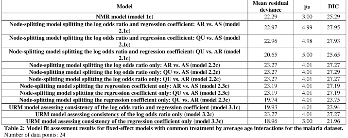
Node-splitting models 11
Table 2 shows model fit assessment results for fixed-effect node-splitting models with 12
common interactions (models 2.1c, 2.2c, 2.3c). The DIC of the NMR model (DIC=25.29) is 13
similar to those of the node-splitting models (DICs 23.75-27.95) indicating that the model is 14
not improved by splitting each node, lending support to the consistency assumptions. 15
16
The results from node-splitting are displayed in Table 3. In the model that assesses 17
consistency of both the log odds ratio and the coefficient (model 2.1c), the log odds ratios for 18
AR vs. AS (-2.3540 95% CrI (-6.7650, 2.0530)) and QU vs. AS (0.4316 95% CrI (0.2833, 19
0.5797)) based on direct evidence differs with those from indirect evidence (i.e. 0.1985 95% 20
CrI (-0.0815, 0.4782) and -2.1000 95% CrI (-6.4180, 2.4430) respectively) because only two 21
trials contribute direct evidence for AR vs. AS and therefore the results are influenced by the 22
vague prior distribution. A similar, but less pronounced, inconsistency is also seen for the 23
corresponding coefficients. Yet, the probability of agreement between direct and indirect 24
comparisons or the log odds ratios (Ps 0.24-0.77). Similar conclusions are drawn from 1
models that split either the log odds ratio or the regression coefficient only (models 2.2c and 2
2.3c). The consistency of the direct and indirect evidence is also supported graphically in 3
Figure 3, which displays the posterior distributions of the centred log odds ratios and 4
regression coefficients and in Figure 4, where the log odds ratio versus average age is plotted. 5
6
URM models 7
Table 2 also displays model fit assessment results for fixed-effect URM models with 8
common interactions (models 3.1c, 3.2c, 3.3c). The DIC of the NMR model (DIC=25.29) is 9
similar to those from the URM models the assess consistency of both the log odds ratio and 10
coefficient (DIC=23.94) or the log odds ratio alone (DIC= 27.27) (models 3.1c and 3.2c) but 11
is slightly higher than that from the model that assesses the coefficient alone (DIC=21.96) 12
(model 3.3c) indicating a possible inconsistency on a coefficient. 13
14
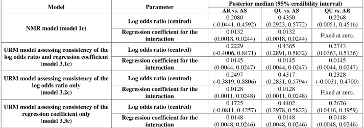
See Table 4 for the results from the NMR model and URM models. The results from the 15
URM models are quite similar to those from the NMR model with the exception of the 16
regression coefficient for QU vs. AR. This difference in the coefficient for QU vs. AR is 17
because of the different assumptions underlying the two models; the NMR model sets the 18
regression coefficients for AR vs. AS and QU vs. AS to be identical (i.e. 0.0132 95% CrI 19
(0.0018, 0.0244)) and the coefficient for QU vs. AR to be zero, whereas all three coefficients 20
are set to be identical in the URM model (i.e. 0.0145 95% CrI (0.0044, 0.0247)). 21
22
Overall, there is evidence of an interaction from the NMR but also evidence of inconsistency; 23
the node-splitting models show evidence of loop inconsistency for the coefficient of QU vs. 24
1
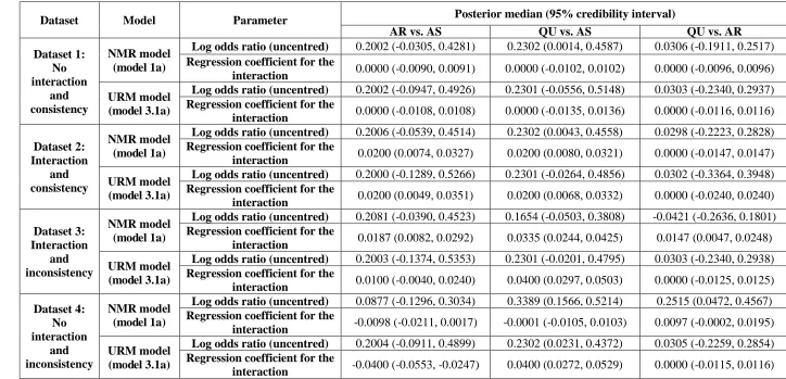
3.3.2. Fabricated datasets 2
Dataset 1: no interaction and consistency. 3
The DICs from each model (models 1a, 2.1a, 3.1a) are similar (8.01-12.00) therefore there is 4
no obvious sign of inconsistency (Table 5). Using the results from node-splitting (model 5
2.1a), the log odds ratios and coefficients based on direct and indirect evidence are very 6
similar and the probabilities of agreement between direct and indirect evidence are practically 7
one (Table 6). The results from the NMR model are also similar to those from the URM 8
model (model 3.1a) (Table 7) indicating consistency. Overall, the NMR model does not show 9
that a treatment by average age interaction exists (Table 7) and there is no evidence of loop 10
inconsistency using node-splitting, or global inconsistency using the URM model. Figure 5, 11
which shows the results from the NMR model and node-splitting models, supports this 12
conclusion. 13
14
Dataset 2: interaction and consistency. 15
The DICs from the models (models 1a, 2.1a, 3.1a) are again similar (8.00-11.99) indicating 16
consistent evidence (Table 5). From node-splitting (model 2.1a), the log odds ratios and the 17
coefficients based on direct and indirect evidence are almost identical and the probabilities of 18
agreement of direct and indirect evidence are practically one (Table 6); Figure 5 shows the 19
results graphically. The URM model (model 3.1a) also gives comparable results to the NMR 20
model (Table 7). In conclusion, the NMR model shows that an interaction exists for AR vs. 21
AS (0.0200 95% CrI (0.0074, 0.0327)) and QU vs. AS (0.0200 95% CrI (0.0080, 0.0321)) 22
(Table 7) and there is no loop inconsistency using node-splitting, or global inconsistency 23
using the URM model. 24
Dataset 3: interaction and inconsistency. 1
The DIC from the NMR model (model 1a) (DIC=47.14) is much higher than those from 2
node-splitting (model 2.1a) and the URM model (model 3.1a) (11.97-11.99) suggesting 3
inconsistency (Table 5). From node-splitting, the log odds ratios based on direct and indirect 4
evidence are comparable but the coefficients for AR vs. AS (0.0100 95% CrI (-0.0039, 5
0.0241)) and QU vs. AS (0.0400 95% CrI (0.0298, 0.0503)) and QU vs. AR (0.0000 95% CrI 6
(-0.0125, 0.0126)) from direct evidence differ from those from indirect evidence (i.e. 0.0400 7
95% CrI (0.0237, 0.0562), 0.0099 95% CrI (-0.0088, 0.0289), and 0.0300 95% CrI (0.0127, 8
0.0474) respectively); the probabilities of agreement of direct and indirect evidence are very 9
high (Ps 0.9982-0.9990) for the log odds ratios and very low for the coefficients (Ps 0.0057-10
0.0062) (Table 6). The URM model also gives results that differ somewhat from those of the 11
NMR model (see Table 7). To summarise, the NMR model shows that an interaction exists 12
for AR vs. AS (0.0187 95% CrI (0.0082, 0.0292)), QU vs. AS (0.0335 95% CrI (0.0244, 0.0425)) 13
and QU vs. AR (0.0147 95% CrI (0.0047, 0.0248)) (Table 7) but there is also loop inconsistency 14
in the size of the underlying coefficients based on direct and indirect evidence that is seen 15
using node-splitting (Figure 5); the URM model identifies global inconsistency. 16
17
Dataset 4: no interaction and inconsistency. 18
The DIC from the NMR model (model 1a) (DIC=188.36) is much higher than those from 19
node-splitting (model 2.1a) and the URM model (model 3.1a) (11.99-12.00) indicating 20
inconsistency (Table 5). Similar to dataset 3, in node-splitting models, the log odds ratios 21
based on direct and indirect evidence are comparable but the coefficients for AR vs. AS (-22
0.0400 95% CrI (-0.0553, -0.0246)) and QU vs. AS (0.0400 95% CrI (0.0273, 0.0529)) and 23
QU vs. AR (0.0000 95% CrI (-0.0115, 0.0116)) from direct evidence differ from those from 24
and 0.0800 95% CrI (0.0600, 0.1000) respectively); the probabilities of agreement of direct 1
and indirect evidence are very high for log odds ratios (Ps 0.9976-1.000) and zero for the 2
coefficients (Table 6). Also, results from the URM model are different from those of the 3
NMR model (see Table 7). Overall, the NMR model shows that no interaction exists (Table 4
7) but there is inconsistency in the direction of the underlying coefficients based on direct and 5
indirect evidence and this trend can be seen using node-splitting (Figure 5); the URM model 6
suggests global inconsistency respectively but these models cannot show the underlying 7
trend. 8
9
4. Discussion 10
We have shown that node-splitting and inconsistency models can be useful for assessing the 11
underlying consistency assumptions of NMR when using aggregate data. Once consistency 12
has been assessed, the analyst must decide which results to present. If the direct and indirect 13
evidence are consistent, the results from the NMR should be reliable. However, the level of 14
heterogeneity (from the NMR or standard pair-wise analyses) and goodness of fit of the NMR 15
should be considered when drawing conclusions from the results. If there is inconsistency, 16
the results from the NMR are questionable and the causes of inconsistency should be 17
considered. In some scenarios, for example, when inconsistency masks an interaction, as 18
shown in Figure 1c and 1g, the results would not be useable. If the original purpose of the 19
NMR was to explore causes of heterogeneity or inconsistency in an NMA and there is no 20
interaction and no inconsistency masking interactions in the NMR, then analysts could 21
proceed by exploring other potentially relative treatment effect modifying covariates or 22
reconsidering the eligibility criteria. 23
Each of the proposed methods has different pros and cons. DBT models assess design and 1
loop consistency and can assess global inconsistency, while node-splitting assesses loop 2
consistency and URM models assess global inconsistency; loop inconsistency is well 3
recognised in the methodological literature but design consistency is a newer concept 4
(Higgins et al., 2012; White et al., 2012). Furthermore, the DBT model requires 5
parameterisation by the analyst therefore, the analyst needs to have a good understanding of 6
the model and parameters. Key advantages of the DBT model and node-splitting is that 7
inconsistency estimates and the probability that direct and indirect evidence agree can be 8
obtained; however, the URM model does not provide such results. Moreover, concerns 9
regarding multiple testing may apply to node-splitting and the DBT models where 10
probabilities are calculated, particularly when a Frequentist approach is taken; therefore, it is 11
important to compare model fit statistics across models, and also to be cautious in 12
interpreting ‘p-values’ making sure to allow for multiple testing. One disadvantage of
node-13
splitting is that, as one model is fitted for every comparison with contributing direct and 14
indirect evidence, many models may need to be fitted which is computationally demanding; 15
whereas only one inconsistency model would need to be applied. 16
17
Ideally, all three approaches (i.e. node-splitting, DBT model, URM model) would be applied 18
to provide a thorough assessment of consistency. However, in practice, the reviewer may 19
select their preferred approach depending on the ease of application in software etc. We 20
recommend that at least one of the global tests (i.e. inconsistency models) and also node-21
splitting are performed. Our preference is node-splitting because estimates from direct and 22
indirect evidence can be found. 23
We proposed and applied methods to trial-level aggregated data in this article. However, it is 1
straightforward to adapt the models to accommodate any type of arm-level outcome data, that 2
is, a summary of the outcome data for each arm of each trial and a covariate value for each 3
trial. To adapt the models, a suitable link function would be chosen and nuisance parameters 4
are included in the model to represent the effect of the baseline treatment in arm 1 of trial i. 5
Further details regarding arm-level network meta-analysis models are given by Dias et al 6
(Dias et al., 2013a) 7
8
Moreover, collection and use of individual patient data is generally advantageous over 9
aggregate data when studying patient-level covariates because they avoid ecological biases 10
(Riley et al., 2008; Riley and Steyerberg, 2010). Yet, it is more common to explore patient-11
level covariates (e.g. patient age) using study-level covariate summaries (e.g. average age of 12
patients) in meta-regression such as in the malaria dataset. However, when using aggregate 13
data, the possibility of confounding and ecological biases should be considered when patient-14
level covariates are explored. 15
16
There are a number of issues that can arise when applying the methods, particularly with 17
aggregate data. Parameter estimation can be a problem with limited data, such that models 18
cannot be fitted at all, interactions exist but cannot be detected, or inconsistency exists but is 19
not found. For instance, when all the trials that contribute to the estimation of a regression 20
coefficient have the same covariate value or when only one trial contributes to a coefficient, 21
this would preclude the use of models with independent interactions but analysts may be able 22
to apply an model with exchangeable or common interactions providing studies that 23
contribute to another basic coefficient have different covariate values. For example, when 24
studies that contribute to results for comparison 2 vs. 1 may all be carried out on the same 1
continent provided that studies that contribute to comparison 3 vs. 1 are located on different 2
continents. Parameter estimation may particularly be a problem when fitting the DBT model 3
because the inconsistency estimates would be imprecise when the number of trials in one or 4
more designs is limited; to overcome this one could assume exchangeability of the 5
inconsistency factors or use informative prior distributions. Similarly, if direct evidence is 6
limited for some comparisons (i.e. few trials or covariate values), the URM model and node-7
splitting models would produce imprecise results and informative prior distributions may 8
need to be used. Ideally any informative prior distributions would be evidence-based by 9
eliciting them from similar meta-analyses or experts’ beliefs. Finally, it is also worth 10
emphasising that no evidence of inconsistency does not automatically imply there is 11
consistency; inconsistency may exist but cannot be detected when data are limited and results 12
are imprecise and therefore arguably the consistency assumptions and the NMR results are 13
questionable. In the same way, in such cases, no evidence of a treatment by covariate 14
interaction does not imply there is truly no interaction. 15
16
Conversely, with abundant data, additional modelling extensions may be feasible. For 17
example, in node-splitting models, we have assumed the between trial variance is the same 18
for direct evidence and indirect evidence, yet it is possible to incorporate two variances, one 19
of each type of evidence. Also, the models could be adapted to include more than one 20
covariate or other variance structures (Lu and Ades, 2009). 21
22
In conclusion, consistency of the assumptions underlying NMR must be assessed when NMR 23
is applied, even when no treatment by covariate interactions are detected. It is possible that 24
reported without assessing the underlying assumptions to determine whether the results are 1
valid and reliable. 2
3
Acknowledgements 4
This research was funded by the Medical Research Council (http://www.mrc.ac.uk/, grant 5
number MR/K021435/1) as part of a career development award in biostatistics awarded to 6
SDo. We are grateful to the two anonymous peer reviewers for their helpful comments. 7
8
References 9
COOPER, N., SUTTON, A., MORRIS, D., ADES, A. & WELTON, N. 2009. Addressing 10
between-study heterogeneity and inconsistency in mixed treatment comparisons: 11
Application to stroke prevention treatments in individuals with non-rheumatic atrial 12
fibrillation. Stat Med, 28, 1861-1881. 13
DIAS, S., SUTTON, A. J., ADES, A. E. & WELTON, N. J. 2013a. Evidence Synthesis for 14
Decision Making 2: A Generalized Linear Modeling Framework for Pairwise and 15
Network Meta-analysis of Randomized Controlled Trials. Med Decis Making, 33, 16
607-617. 17
DIAS, S., SUTTON, A. J., WELTON, N. J. & ADES, A. E. 2013b. Evidence Synthesis for 18
Decision Making 3: Heterogeneity—Subgroups, Meta-Regression, Bias, and Bias-19
Adjustment. Med Decis Making, 33, 618-640. 20
DIAS, S., WELTON, N. J., CALDWELL, D. M. & ADES, A. E. 2010. Checking consistency 21
in mixed treatment comparison meta-analysis. Stat Med, 29, 932-944. 22
DIAS, S., WELTON, N. J., SUTTON, A. J., CALDWELL, D. M., LU, G. & ADES, A. E. 23
2013c. Evidence Synthesis for Decision Making 4: Inconsistency in Networks of 24
DONEGAN, S., WILLIAMSON, P., D'ALESSANDRO, U. & TUDUR SMITH, C. 2013a. 1
Assessing key assumptions of network meta-analysis: a review of methods. Res Syn 2
Meth, 4, 291-323. 3
DONEGAN, S., WILLIAMSON, P., D'ALESSANDRO, U., GARNER, P. & TUDUR 4
SMITH, C. 2013b. Combining individual patient data and aggregate data in mixed 5
treatment comparison meta-analysis: Individual patient data may be beneficial if only 6
for a subset of trials. Stat Med, 32, 914-930. 7
DONEGAN, S., WILLIAMSON, P., D'ALESSANDRO, U. & TUDUR SMITH, C. 2012. 8
Assessing the consistency assumption by exploring treatment by covariate 9
interactions in mixed treatment comparison meta-analysis: individual patient-level 10
covariates versus aggregate trial-level covariates. Stat Med, 31, 3840-3857. 11
ESU, E., EFFA, E. E., OPIE, O. N., UWAOMA, A. & MEREMIKWU, M. M. 2014. 12
Artemether for severe malaria. Cochrane Database Syst Rev, 9, CD010678.. 13
HIGGINS, J. & WHITEHEAD, A. 1996. Borrowing strength from external trials in a meta-14
analysis. Stat Med, 15, 2733-49. 15
HIGGINS, J. P. T., JACKSON, D., BARRETT, J. K., LU, G., ADES, A. E. & WHITE, I. R. 16
2012. Consistency and inconsistency in network meta-analysis: concepts and models 17
for multi-arm studies. Res Syn Meth, 3, 98–110. 18
JACKSON, D., BARRETT, J. K., RICE, S., WHITE, I. R. & HIGGINS, J. P. T. 2014. A 19
design-by-treatment interaction model for network meta-analysis with random 20
inconsistency effects. Stat Med, 33, 3639-3654. 21
JACKSON, D., BODDINGTON, P. & WHITE, I. R. 2016. The design-by-treatment 22
interaction model: a unifying framework for modelling loop inconsistency in network 23
JANSEN, J. & COPE, S. 2012. Meta-regression models to address heterogeneity and 1
inconsistency in network meta-analysis of survival outcomes. BMC Med Res 2
Methodol, 12, 152. 3
JANSEN, J. P. 2012. Network meta-analysis of individual and aggregate level data. Res Syn 4
Meth, 3, 177-190. 5
LAW, M., JACKSON, D., TURNER, R., RHODES, K. & VIECHTBAUER, W. 2016. Two 6
new methods to fit models for network meta-analysis with random inconsistency 7
effects. BMC Med Res Methodol, 16, 87. 8
LU, G. & ADES, A. 2004. Combination of direct and indirect evidence in mixed treatment 9
comparisons. Stat Med, 23, 3105 - 3124. 10
LU, G. & ADES, A. 2006. Assessing evidence inconsistency in mixed treatment 11
comparisons. J Am Stat Assoc 101, 447-459. 12
LU, G. & ADES, A. 2009. Modeling between-trial variance structure in mixed treatment 13
comparisons. Biostatistics, 10, 792-805. 14
MARSHALL, E. & SPIEGELHALTER, D. 2007. Identifying outliers in Bayesian 15
hierarchical models: a simulation-based approach. Bayesian Anal, 2, 409-444. 16
NIXON, R. M., BANSBACK, N. & BRENNAN, A. 2007. Using mixed treatment 17
comparisons and meta-regression to perform indirect comparisons to estimate the 18
efficacy of biologic treatments in rheumatoid arthritis. Stat Med, 26, 1237-54. 19
RILEY, R. D., LAMBERT, P. C., STAESSEN, J. A., WANG, J., GUEYFFIER, F., THIJS, 20
L. & BOUTITIE, F. 2008. Meta-analysis of continuous outcomes combining 21
individual patient data and aggregate data. Stat Med, 27, 1870-1893. 22
RILEY, R. D. & STEYERBERG, E. W. 2010. Meta-analysis of a binary outcome using 23
SALANTI, G., MARINHO, V. & HIGGINS, J. P. T. 2009. A case study of multiple-1
treatments meta-analysis demonstrates that covariates should be considered. J Clin 2
Epidemiol, 62, 857-864. 3
SARAMAGO, P., SUTTON, A. J., COOPER, N. J. & MANCA, A. 2012. Mixed treatment 4
comparisons using aggregate and individual participant level data. Stat Med, 31, 5
3516-3536. 6
SINCLAIR, D., DONEGAN, S., ISBA, R. & LALLOO DAVID, G. 2012. Artesunate versus 7
quinine for treating severe malaria. Cochrane Database Syst Rev, 6, CD005967. 8
SPIEGELHALTER, D. J., BEST, N. G., CARLIN, B. P. & VAN DER LINDE, A. 2002. 9
Bayesian measures of model complexity and fit. Med Decis Making, 64, 583-639. 10
THOMPSON, S. & SHARP, S. 1999. Explaining heterogeneity in meta-analysis: a 11
comparison of methods. Stat Med, 18, 2693 - 2708. 12
THOMPSON, S. G. 1994. Systematic Review: Why sources of heterogeneity in meta-13
analysis should be investigated. BMJ, 309, 1351-1355. 14
THOMPSON, S. G., HIGGINS, J. P. T. 2002. How should meta-regression analyses be 15
undertaken and interpreted? Stat Med, 21, 1559-1573. 16
TUDUR SMITH, C., MARSON, A., CHADWICK, D. & WILLIAMSON, P. 2007. Multiple 17
treatment comparisons in epilepsy monotherapy trials. Trials, 8, 34. 18
VAN VALKENHOEF, G., DIAS, S., ADES, A. E. & WELTON, N. J. 2016. Automated 19
generation of node-splitting models for assessment of inconsistency in network meta-20
analysis. Res Syn Meth, 7, 80-93. 21
WHITE, I. R., BARRETT, J. K., JACKSON, D. & HIGGINS, J. P. T. 2012. Consistency and 22
inconsistency in network analysis: model estimation using multivariate meta-23
WORLD HEALTH ORGANISATION 2015. Guidelines for the treatment of malaria. Third 1
edition ed. 2
Models including independent treatment by
covariate interactions
Models including exchangeable treatment by
covariate interactions
Models including common treatment by covariate
interactions
NMR models Model 1a Model 1b Model 1c
Node-splitting
models
Models splitting the relative treatment effect and the regression
coefficient for the interaction.
Model 2.1a Model 2.1b Model 2.1c
Models splitting the relative
treatment effect only. Model 2.2a Model 2.2b Model 2.2c
Models splitting the regression
coefficient for the interaction only. Model 2.3a Model 2.3b Model 2.3c
URM models
Models assessing consistency of the relative treatment effect and the
regression coefficient for the interaction.
Model 3.1a Model 3.1b Model 3.1c
Models assessing consistency of the
relative treatment effect only. Model 3.2a Model 3.2b Model 3.2c
Models assessing consistency of the regression coefficient for the
interaction only.
Model 3.3a Model 3.3b Model 3.3c
DBT models
Models assessing consistency of the relative treatment effect and the
regression coefficient for the interaction.
Model 4.1a Model 4.1b Model 4.1c
Models assessing consistency of the
relative treatment effect only. Model 4.2a Model 4.2b Model 4.2c
Models assessing consistency of the regression coefficient for the
interaction only.
Model 4.3a Model 4.3b Model 4.3c
Model Mean residual
deviance pD DIC
NMR model (model 1c) 22.29 3.00 25.29
Node-splitting model splitting the log odds ratio and regression coefficient: AR vs. AS (model
2.1c) 22.97 4.99 27.95
Node-splitting model splitting the log odds ratio and regression coefficient: QU vs. AS (model
2.1c) 22.96 4.98 27.93
Node-splitting model splitting the log odds ratio and regression coefficient: QU vs. AR (model
2.1c) 20.65 5.00 25.65
[image:34.842.64.780.74.358.2]Node-splitting model splitting the log odds ratio only: AR vs. AS (model 2.2c) 23.27 4.01 27.27 Node-splitting model splitting the log odds ratio only: QU vs. AS (model 2.2c) 23.27 4.01 27.29 Node-splitting model splitting the log odds ratio only: QU vs. AR (model 2.2c) 23.27 4.01 27.27 Node-splitting model splitting the regression coefficient only: AR vs. AS (model 2.3c) 23.19 4.01 27.19 Node-splitting model splitting the regression coefficient only: QU vs. AS (model 2.3c) 23.19 4.01 27.19 Node-splitting model splitting the regression coefficient only: QU vs. AR (model 2.3c) 19.74 4.01 23.75 URM model assessing consistency of the log odds ratio and regression coefficient (model 3.1c) 19.93 4.01 23.94 URM model assessing consistency of the log odds ratio only (model 3.2c) 23.27 4.01 27.27 URM model assessing consistency of the regression coefficient only (model 3.3c) 18.96 3.00 21.96 Table 2: Model fit assessment results for fixed-effect models with common treatment by average age interactions for the malaria dataset. Number of data points: 24
Model type Parameter Evidence Posterior median (95% credibility interval), P
AR vs. AS QU vs. AS QU vs. AR
Splitting the log odds ratio and regression coefficient (model 2.1c)
Log odds ratio (centred)
Direct -2.3540 (-6.7650, 2.0530)* 0.4316 (0.2833, 0.5797) 0.2882 (0.0449, 0.5315) Indirect 0.1985 (-0.0815, 0.4782) -2.1000 (-6.4180, 2.4430)* 0.1825 (-0.4751, 0.8419)
IE, P -2.5510 (-6.9740, 1.8710), P=0.26
2.5330 (-2.0150, 6.8540), P=0.26
0.1055 (-0.5990, 0.8089), P=0.77
Regression coefficient for the interaction
Direct 0.1738 (-0.0974, 0.4451) 0.0126 (0.0006, 0.0245) 0.0191 (-0.0008, 0.0387) Indirect 0.0126 (0.0007, 0.0245) 0.1728 (-0.1048, 0.4376) Fixed at zero
IE, P 0.1613 (-0.1100, 0.4327), P=0.25
-0.1603 (-0.4253, 0.1173), P=0.24
0.0191 (-0.0008, 0.0387), P=0.06
Splitting the log odds ratio only (model 2.2c)
Log odds ratio (centred)
Direct 0.2495 (-0.3804, 0.8815) 0.4320 (0.2837, 0.5804) 0.2328 (-0.0031, 0.4700) Indirect 0.1994 (-0.0821, 0.4787) 0.4824 (-0.1946, 1.1600) 0.1816 (-0.4797, 0.8403)
IE, P 0.0512 (-0.6481, 0.7515), P=0.89
-0.0499 (-0.7523, 0.6552), P=0.89
0.0521 (-0.6518, 0.7545), P=0.89
Regression coefficient
for the interaction All 0.0129 (0.0011, 0.0248) 0.0129 (0.0011, 0.0248) Fixed at zero
Splitting the regression coefficient
only (model 2.3c)
Log odds ratio
(centred) All 0.1890 (-0.0918, 0.4673) 0.4283 (0.2793, 0.5747) 0.2746 (0.0469, 0.5033)
Regression coefficient for the interaction
Direct 0.0195 (-0.0210, 0.0603) 0.0126 (0.0007, 0.0245) 0.0188 (-0.0007, 0.0385) Indirect 0.0125 (0.0007, 0.0245) 0.0194 (-0.0210, 0.0601) Fixed at zero
IE, P 0.0070 (-0.0358, 0.0500), P=0.75
-0.0068 (-0.0498, 0.0357), P=0.76
0.0188 (-0.0007, 0.0385), P=0.06
Table 3: Results from fixed-effect node-splitting models including common treatment by average age interactions for the malaria dataset.
[image:35.842.67.729.86.404.2]Model Parameter Posterior median (95% credibility interval)
AR vs. AS QU vs. AS QU vs. AR
NMR model (model 1c)
Log odds ratio (centred) 0.2080 (-0.0441, 0.4592)
0.4350 (0.2923, 0.5772)
0.2268 (0.0051, 0.4516) Regression coefficient for the
interaction
0.0132 (0.0018, 0.0244)
0.0132
(0.0018, 0.0244) Fixed at zero.
URM model assessing consistency of the log odds ratio and regression coefficient
(model 3.1c)
Log odds ratio (centred) 0.2229 (-0.4006, 0.8471)
0.4365 (0.2891, 0.5832)
0.2743 (0.0363, 0.5136) Regression coefficient for the
interaction 0.0145 (0.0044, 0.0247) 0.0145 (0.0044, 0.0247) 0.0145 (0.0044, 0.0247)
URM model assessing consistency of the log odds ratio only
(model 3.2c)
Log odds ratio (centred) 0.2497 (-0.3819, 0.8806)
0.4317 (0.2831, 0.5794)
0.2328 (-0.0031, 0.4700) Regression coefficient for the
interaction
0.0128 (0.0011, 0.0248)
0.0128
(0.0011, 0.0248) Fixed at zero.
URM model assessing consistency of the regression coefficient only
(model 3.3c)
Log odds ratio (centred) 0.1725 (-0.0811, 0.4257)
0.4402 (0.2978, 0.5822)
0.2676 (0.0416, 0.4959) Regression coefficient for the
[image:36.842.65.778.73.325.2]Dataset Model
Mean residual deviance
pD DIC
Dataset 1: No interaction and consistency
NMR model (model 1a) 4.00 4.00 8.01
Node-splitting model: AR vs. AS (model 2.1a) 6.00 6.00 12.00
Node-splitting model: QU vs. AS (model 2.1a) 5.99 5.99 11.98
Node-splitting model: QU vs. AR (model 2.1a) 5.99 5.99 11.98
URM model (model 3.1a) 5.99 5.99 11.97
Dataset 2: Interaction and consistency
NMR model (model 1a) 4.00 4.00 8.00
Node-splitting model: AR vs. AS (model 2.1a) 6.00 6.00 11.99
Node-splitting model: QU vs. AS (model 2.1a) 5.99 5.99 11.99
Node-splitting model: QU vs. AR (model 2.1a) 5.99 5.99 11.97
URM model (model 3.1a) 5.98 5.98 11.97
Dataset 3: Interaction and inconsistency
NMR model (model 1a) 43.14 3.99 47.14
Node-splitting model: AR vs. AS (model 2.1a) 5.99 5.99 11.99
Node-splitting model: QU vs. AS (model 2.1a) 6.00 6.00 11.99
Node-splitting model: QU vs. AR (model 2.1a) 5.98 5.98 11.97
URM model (model 3.1a) 5.99 5.99 11.97
Dataset 4: No interaction and inconsistency
NMR model (model 1a) 184.36 4.00 188.36
Node-splitting model: AR vs. AS (model 2.1a) 6.00 6.00 12.00
Node-splitting model: QU vs. AS (model 2.1a) 5.99 5.99 11.99
Node-splitting model: QU vs. AR (model 2.1a) 6.00 6.00 11.99
[image:37.842.65.776.72.413.2]URM model (model 3.1a) 5.99 5.99 11.98
Table 5: Model fit assessment results for fixed-effect models assessing consistency of both the log odds ratio and regression coefficient with independent treatment by average age interactions for the fabricated datasets.
Number of data points: 30
Dataset Parameter Evidence Posterior median (95% credibility interval), P
AR vs. AS QU vs. AS QU vs. AR
Dataset 1: No interaction
and consistency
Log odds ratio (uncentred)
Direct 0.1997 (-0.0948, 0.4949) 0.2302 (-0.0566, 0.5139) 0.0298 (-0.2356, 0.2937)
Indirect 0.2001 (-0.1865, 0.5902) 0.2306 (-0.1642, 0.6265) 0.0297 (-0.3799, 0.4398)
IE, P -0.0007 (-0.4870, 0.4894), P=0.9974 -0.0004 (-0.4879, 0.4875), P=0.9986 -0.0002 (-0.4891, 0.4886), P=0.9990
Regression coefficient for the
interaction
Direct 0.0000 (-0.0107, 0.0109) 0.0000 (-0.0135, 0.0136) 0.0000 (-0.0115, 0.0116)
Indirect 0.0000 (-0.0178, 0.0178) 0.0000 (-0.0158, 0.0158) 0.0000 (-0.0174, 0.0174)
IE, P 0.0000 (-0.0210, 0.0208),
P=0.9980
0.0000 (-0.0208, 0.0209), P=0.9980
0.0000 (-0.0208, 0.0209), P=0.9982
Dataset 2: Interaction
and consistency
Log odds ratio (uncentred)
Direct 0.1992 (-0.1284, 0.5285) 0.2300 (-0.0268, 0.4852) 0.0301 (-0.3372, 0.3941)
Indirect 0.1998 (-0.2432, 0.6460) 0.2304 (-0.2614, 0.7213) 0.0299 (-0.3886, 0.4447)
IE, P -0.0007 (-0.5528, 0.5534), P=0.9980 -0.0001 (-0.5549, 0.5537), P=0.9998 -0.0003 (-0.5542, 0.5548), P=0.9996
Regression coefficient for the
interaction
Direct 0.0200 (0.0049, 0.0352) 0.0200 (0.0069, 0.0333) 0.0000 (-0.0239, 0.0240)
Indirect 0.0200 (-0.0073, 0.0473) 0.0199 (-0.0084, 0.0485) 0.0000 (-0.0200, 0.0201)
IE, P 0.0000 (-0.0313, 0.0312),
P=0.9974
0.0001 (-0.0315, 0.0313), P=0.9954
0.0000 (-0.0311, 0.0313), P=1.0000
Dataset 3: Interaction
and inconsistency
Log odds ratio (uncentred)
Direct 0.2000 (-0.1389, 0.5372) 0.2301 (-0.0208, 0.4796) 0.0301 (-0.2355, 0.2937)
Indirect 0.1999 (-0.1619, 0.5649) 0.2304 (-0.1985, 0.6584) 0.0299 (-0.3924, 0.4492)
IE, P 0.0003 (-0.4955, 0.4950), P=0.9990 -0.0006 (-0.4948, 0.4955), P=0.9982 -0.0004 (-0.4971, 0.4983), P=0.9986
Regression coefficient for the
interaction
Direct 0.0100 (-0.0039, 0.0241) 0.0400 (0.0298, 0.0503) 0.0000 (-0.0125, 0.0126)
Indirect 0.0400 (0.0237, 0.0562) 0.0099 (-0.0088, 0.0289) 0.0300 (0.0127, 0.0474)
IE, P -0.0300 (-0.0515, -0.0088), P=0.0059 0.0301 (0.0085, 0.0514), P=0.0062 -0.0300 (-0.0515, -0.0086), P=0.0057
Dataset 4: No interaction
and inconsistency
Log odds ratio (uncentred)
Direct 0.2002 (-0.0926, 0.4908) 0.2300 (0.0222, 0.4360) 0.0297 (-0.2260, 0.2863)
Indirect 0.2000 (-0.1290, 0.5298) 0.2300 (-0.1569, 0.6178) 0.0301 (-0.3279, 0.3866)
IE, P -0.0003 (-0.4376, 0.4397), P=0.9990 -0.0007 (-0.4393, 0.4399), P=0.9976 0.0000 (-0.4398, 0.4398), P=1.0000
Regression coefficient for the
interaction
Direct -0.0400 (-0.0553, -0.0246) 0.0400 (0.0273, 0.0529) 0.0000 (-0.0115, 0.0116)
Indirect 0.0399 (0.0227, 0.0574) -0.0400 (-0.0591, -0.0208) 0.0800 (0.0600, 0.1000)
IE, P -0.0799 (-0.1031, -0.0571), P=0.0000 0.0800 (0.0568, 0.1030), P=0.0000 -0.0800 (-0.1031, -0.0569), P=0.0000
Table 6: Results from fixed-effect node-splitting models splitting both the log odds ratio and regression coefficient including independent treatment by average age interactions (model 2.1a) for the fabricated datasets.
[image:38.842.70.768.71.476.2]