An autonomous surface discontinuity detection and quantification method by digital image correlation and phase congruency

This is a repository copy of An autonomous surface discontinuity detection and quantification method by digital image correlation and phase congruency. White Rose Research Online URL for this paper:

http://eprints.whiterose.ac.uk/116800/ Version: Accepted Version

Article:

Cinar, A.F., Barhli, S.M., Hollis, D. et al. (4 more authors) (2017) An autonomous surface discontinuity detection and quantification method by digital image correlation and phase congruency. Optics and Lasers in Engineering, 96. pp. 94-106. ISSN 0143-8166

https://doi.org/10.1016/j.optlaseng.2017.04.010

Article available under the terms of the CC-BY-NC-ND licence (https://creativecommons.org/licenses/by-nc-nd/4.0/

eprints@whiterose.ac.uk https://eprints.whiterose.ac.uk/ Reuse

This article is distributed under the terms of the Creative Commons Attribution-NonCommercial-NoDerivs (CC BY-NC-ND) licence. This licence only allows you to download this work and share it with others as long as you credit the authors, but you can’t change the article in any way or use it commercially. More

information and the full terms of the licence here: https://creativecommons.org/licenses/

Takedown

If you consider content in White Rose Research Online to be in breach of UK law, please notify us by

An autonomous surface discontinuity detection and

quantification method by digital image correlation and phase

congruency*

A.F. Cinar

, S.M. Barhli

, D. Hollis

, M. Flansbjer

, R.A. Tomlinson

, T.J. Marrow

,

M. Mostafavi

1

Department of Mechanical Engineering, University of Sheffield, UK

2

Department of Materials, University of Oxford, UK

3

LaVision UK

4

RISE Research Institutes of Sweden, Mechanics Research, SE

5

Department of Mechanical Engineering, University of Bristol, UK

Abstract

Digital image correlation has been routinely used to measure full-field displacements in many areas of solid mechanics, including fracture mechanics. Accurate segmentation of the crack path is needed to study its interaction with the microstructure and stress fields, and studies of crack behaviour, such as the effect of closure or residual stress in fatigue, require data on its opening displacement. Such information can be obtained from any digital image correlation analysis of cracked components, but it collection by manual methods is quite onerous, particularly for massive amounts of data. We introduce the novel application of Phase Congruency to detect and quantify cracks and their opening. Unlike other crack detection techniques, Phase Congruency does not rely on adjustable threshold values that require user interaction, and so allows large datasets to be treated autonomously. The accuracy of the Phase Congruency based algorithm in detecting cracks is evaluated and compared with conventional methods such as Heaviside function fitting. As Phase Congruency is a displacement-based method, it does not suffer from the noise intensification to which gradient-based methods (e.g. strain thresholding) are susceptible. Its application is demonstrated to experimental data for cracks in quasi-brittle (Granitic rock) and ductile (Aluminium alloy) materials.

Keywords

Digital image correlation, fracture mechanics, crack, phase congruency, segmentation

*

Corresponding Author: Mahmoud Mostafavi, Department of Mechanical Engineering, Queen’s Building, University Walk, Bristol, UK BS8 1TR

Email: m.mostafavi@bristol.ac.uk

1

_!

Introduction

Observing the interaction of cracks with the encompassing microstructure of engineering materials is a critical process in structural integrity. Quantitative image-based techniques, such as Digital Image Correlation (DIC), have gained in popularity due to the advances made in the recent years with cheaper CCDs (Charged Coupled Device) and computational power. However, with the advancement of data acquisition, users are faced with the burdensome task of rigorous analysis of large volumes of data, which require user judgement and intervention. The ability to detect and quantify features such as cracks and their associated parameters, such as dimension, from many images is becoming a critical task.

Most approaches to identify cracks in digital images use edge detection methods such as global and local grey-scale intensity thresholding. These require human interaction to be optimal [1, 2]. For instance, Ikhlas et al. [3] presented a study of different edge detection techniques including wavelet transform and Fast Fourier Transform (FFT) to identify cracks in bridges, concluding that wavelet transform is more reliable than other methods. However, the method is based on a chosen threshold value, which is a parameter crucial to its performance. Tomoyuki et al. [4] proposed a fast crack detection method, applied to concrete surfaces, that was based on percolation-based image processing; their quantitative analysis showed this to be computationally more efficient that the wavelet approach but at the cost of precision. Additionally, these methods assume that the crack is sufficiently open enough to be detectable in the image. This inherently limits these methods’ accuracy to a pixel at best. However, there are image analysis techniques that have sub-pixel accuracy. They track the surface displacement of the features near the discontinuity and therefore can detect cracks that are not otherwise visible in the raw image [5]. For example, Avril et al. [6] introduced a method of detecting surface discontinuities and calculation of the crack width with sub-pixel precision, using a grid that is periodically spaced on the surface of the cracked body and with the aid of Windowed discrete Fourier transform to calculate the phase shift between the cracked faces.

DIC is now the most widely used optical based method in fracture mechanics. Introduced in the 1980s by Peters and Ranson [7-9], DIC is a full field non-contact displacement measurement method that is relatively easy to set-up and provides high resolution and high spatial resolution. The fundamental principle of DIC is to compare grey-scale images of an object surface captured before and after deformation; these are referred to as the reference and deformed image, respectively. Conventionally, the reference image is divided into interrogating windows or subsets that are matched (or tracked) in the deformed image, using a shape function, to obtain the displacement of each interrogation window. Higher order shape functions can be used to obtain improved displacement approximations but usually first or second order provides sufficient accuracy [10]. Different matching procedures can be used to search and evaluate the similarity of the grey-scale pattern [11]. This study used the iterative least square method (ILS) method, proposed by Pan et al [12] and incorporated in LaVision Davis Strain Master Code [13].

between the two fields finds the optimal stress intensity factor that describes the measurement. This forces experimental data to fit a theoretical model and neglects possible incompatibilities. Critically, this family of methods are quite sensitive to accurate identification of the crack tip location [19], which can be computationally difficult or conceptually impossible, in the case of diffusive damage zones, to find [20].

An alternative method is to calculate energy release rate via a contour integral method, such as the J-integral [21], to obtain the difference between the work of traction exerted on a finite volume of material and the elastic strain energy in that volume in the presence of a crack. The rate of this difference with respect to an infinitesimal increase in the crack length is the strain energy release rate associated with a crack. This strain energy release rate can be related to an equivalent stress intensity factor [22]. Becker et al. [16] introduced a method to calculate J-integral as an area integral using digital image correlation displacement field measurements and the finite element method. A critical point in this [16] and similar techniques [18, 23, 24], is that although there is less sensitivity to the crack tip position, the crack geometry needs to be identified correctly as the contour integral should be carried out on a path that starts and ends on traction free surfaces, i.e. the crack face.

The displacement discontinuity across the faces of the crack, known as the crack opening displacement (COD), has also been used for both elastic and elastic-plastic materials as a crack quantifying parameter [25-27], as it has a direct relationship with the stress intensity factor or J-integral. It is applied in engineering standards less frequently (e.g. see BS7910) as direct measurements can be difficult to obtain reliably [28]. It can, however, be quantified by digital image correlation [29-35] of surface observations. For instance, Mekky et al [36] have presented a methodology to calculate COD profile along the crack by a least-square method to evaluate the opening displacement by fitting the displacements from opposite sides of the crack. Wells et al [37] fitted a Heaviside function to the discontinuity across the crack faces to located the boundaries of the crack faces. However, most methods in the literature simply requires the user to manually select virtual displacement gauges across the crack faces [38-40], the halfway points between them was used to define the crack path [23, 33, 41, 42].

In a typical experimental study to quantify cracks and their interaction with the microstructure, hundreds of images may be recorded of a growing crack in a complex microstructure; the task of manual segmentation of the crack [43] can be a major obstacle. In this paper, we present a novel algorithmic method of obtaining the crack path and its opening displacement profile autonomously and reliably. We evaluate the theoretical accuracy of the algorithm and compare it with two other crack segmentation algorithms: strain thresholding and Heaviside function fitting. We investigate the reliability of the algorithm using virtual experiments and then show its strength in experimental conditions by examining its performance and speed in case studies on two classes of materials: quasi-brittle and ductile.

2

_!

Algorithm

and 5 pixel crack mouth opening displacements (CMOD). Each image is deformed using the theoretical displacement field around a linear elastic crack, presented by Williams [44]; see section 3. Theoretical study. The reference (closed crack in either case) and deformed (open crack) images were analysed with the LaVision Davis 8.2.6 software [13] using an iterative least squares algorithm [12] with subset size 31 pixels with 75% overlap (Step size 8 pixels). The resultant opening displacement fields are shown in Figure 1c and d and those of opening strain in Figure 1e and f. For the CMOD of 5 pixels the image artefact that represents the crack is visible. It introduces displacement errors close to the crack faces due to the discontinuity in the deformed image that was not present in the reference image. Because of this artefact, in the presence of a crack, the conventional DIC algorithms achieve poor correlation for subsets close to the crack faces. This is because the subsets used for correlation can only capture continuous deformations from the reference of the deformed image [23, 24].

Most crack detection algorithms apply gradient-based (i.e. strain) methods to obtain the path of the crack [30, 31, 34, 45]. Such methods rely on defining a threshold value, which may need to vary between analyses due to change in the quality of the data or the images; for example, the levels of strain that define the crack in Figure 1e and f are an order of magnitude different. Gradient-based methods are sensitive to the gradient magnitude, smoothness and magnification, and do not localize accurately [46]. Other crack detection methods have used fitting the displacement step into a model such as a Heaviside function [32], which are also dependent on the step threshold value.

Phase Congruency (PC) is a relatively new technique in image analysis that uses Phase information† to detect and identify edges and corners in digital images [47]. There have been studies that suggest that phase information is a psychological representation of how human visual system perceives edge like features [48]. Rather than defining features directly at points with sharp changes in value, phase congruency dictates the features, that are perceived at points, where the Fourier components are maximal in phase with each another [49-52]. PC returns a dimensionless quantity that is invariant to contrast and scale and therefore does not suffer from the thresholding problems of other crack segmentation methods [46]. Unlike gradient-based feature detection algorithms, which can only detect step features, PC detects features at all phase angles, and not just step features that have a phase angle of 0 or 180°. Together with the illumination invariance with and accurate localisation [46, 47], PC makes an ideal method for detecting local discontinuities in the displacement fields that are the signature of cracks. The mathematical representation of phase congruency is described in Appendix A.

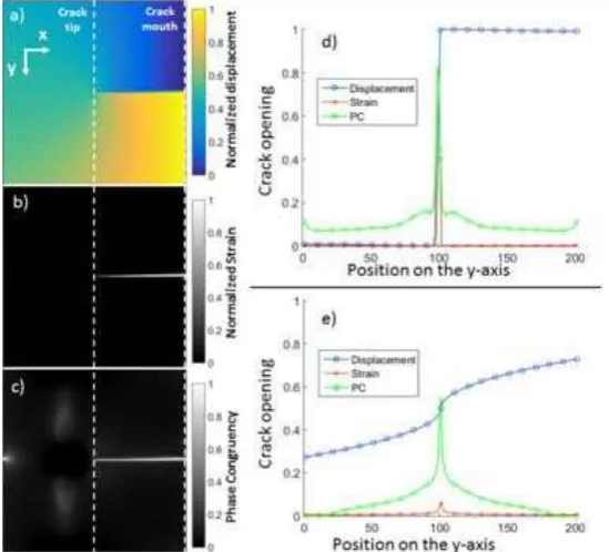
We use Kovesi's representation of PC [46] equipped with noise compensation features based on log-Gabor transfer function, and also employ monogenic filters [53]. Lijuan et al. [54] showed that monogenic filters require less time and memory space compared to log-Gabor filters and they improve the accuracy and sensitivity of PC calculation to noise. An example of a PC outcome is shown in Figure 2; it is a PC analysis of a dataset similar to those presented in Figure 1 but with a crack mouth opening displacement of 1 pixel. The variation of phase congruency, opening displacement, and opening strain is presented along two line profiles vertical to the crack path: at the crack mouth and at the crack tip; the opening strain is normalised with respect to maximum strain. The normalised strain and displacement profiles

†

deteriorate close to the crack tip, while the phase congruency remains consistent. The value of the phase congruency at location (", $), &' (", $), varies from a maximum of 1 (indicating a very significant feature) to 0 (i.e. no significance.

The algorithm proposed to segment the crack autonomously (see the graphical presentation in Figure 3) is as follows: PC analysis is run on the DIC-measured displacement field of a cracked specimen, followed by an active contour segmentation. Active contour segmentation, also known as the Snake algorithm [55, 56], is an iterative feature identification technique based on an energy-minimizing spline [55]. Lankton’s region-based active contour segmentation [57] was used in this work to obtain the segmentation of the local discontinuity detected by PC. The active contour algorithm requires three input parameters: input image; the number of iterations, and the initial mask. In our study the input image is the PC map; the number of iterations is decided when the segmentation converges, and the initial mask is selected by an automatic process, using the displacement map normal to the crack. This initial mask may be an overshot‡ or an undershot§; the active contour algorithm decreases or increases the mask until an optimum is reached. It was noticed during the analyses that undershot initial mask performance is much more reliable.

To produce an undershot initial mask of the crack, the displacement map is smoothed using a bilateral filter [58], which is an image-processing tool that removes noise from images while preserving edges [59]. The next step is the Sobel operator [60], which is an edge detection filter, that produces a map of all the edges in the image; this includes edges produced by noise and the discontinuity. Next, the Hough transform is used to find the co-ordinates of the longest line, which assumed to be the crack, in the edge map. The Hough transform is a feature detection technique that can isolate features of a particular shape within an image [61]. The detected longest line is the longest discontinuity in the displacement map because the edge-preserving filter applied previously removes most of the displacement noise, leaving only sporadic noise that appears as short edges [45]. The detected longest line is an undershot of the discontinuity detected by PC and therefore is used as an initial mask.

It is then possible to quantify the crack parameters: the crack opening displacement (COD) profile** and the crack path††. The segmentation provides a map of the PC detected feature of the discontinuity. Points at the boundary of the segmentation are considered to be the crack faces. These points can be used to calculate both COD and the crack path. The crack opening displacement is the displacement difference between the two faces of the crack and the crack path is the mid-point between the crack faces.

3

_!

Theoretical study

In this section a theoretical displacement field of a crack in an infinite linear elastic plate is used to deform a 2024x2024 pixel synthetic image of a typical speckle pattern to quantify the accuracy of the algorithm presented in the previous section. Crack parameters such as crack opening displacement profile ) " , crack path * " , and crack length are known parameters in the synthetic image and can readily be compared with those calculated by the PC-based crack detection method. To evaluate the algorithm’s robustness to noise, zero-mean additive

‡

Initial mask is a superset of the crack §

Initial mask is a subset of the crack **

Width of the crack ††

white Gaussian noise [62] is added to the theoretical displacement field with an incremental standard deviation of Gaussian noise and the effects were studied.

The continuum mechanics solution of the displacement field ahead of a crack in an elastic medium is an asymptotic function [18]. Assuming only the first term of the asymptotic function for a crack along the horizontal direction i.e. x axis shown in Figure 2a, the opening displacement, +$, around the crack as a function of the far field applied stress, ,, can be presented by:

+$ (-, .) = , 01

23

-20 sin (

1

2.) 8 + 1 − 2cos

=₍1

2.) (1)

where 3 is the shear modulus and - and . are radial and phase distance from the crack tip and a is the crack length. The origin of this "$ – coordinate system is at the crack tip. The crack opening displacement )(") is calculated by [63]:

Displacement in crack plane . = 0 ; - = 1 − "

+$ = 1 + ? 8 + 1

@

,

2 21(1 − ") (2)

) " = 2+$ " = 1 + ? 8 + 1

@ , 21(1 − ") (3)

Where A is Poisson’s ratio and 8 = 3 − 4A for the plane strain condition.

The theoretical +$ displacement field and COD is constructed with an arbitrary Young’s modulus of 8 GPa and Poisson’s ratio of 0.3. It should be noted that only the singular term of displacement field is used in this study. As the distance from the crack tip increases the contribution of non-singular terms increases [64] and the crack opening displacement calculated by Eq. 3 is no longer valid. However, the aim of this theoretical study is to compare a known crack opening displacement with that calculated by our algorithm to estimate its accuracy and therefore the unrepresentativeness of the selected field has no effect on the estimated accuracy.

It is a challenging task to accurately model typical experimental DIC noises as there are many different factors that contribute to the uncertainty in the measured displacement field. Hence to simulate the effects of noise in displacement field, additive Gaussian white noise with mean value of 0, and different increments of standard deviation were added to the theoretical displacement field. The standard deviation ,_D and percent additive noise, Γ_F are introduced with the following form:

Γ_F= ,D

(∆+$)×100 (4)

∆+$ is the range of the displacement field (i.e. the difference between the maximum and minimum displacements in the analysis), and has value 1 as +$ is normalised. The simulated

ΓF ranges from 0% (no noise) to 10% with increments of 0.01%. For a predefined value of ΓF,

,D is the standard deviation of a normal distribution from which a random value is extracted,

J K, L , and added to the displacement field as shown in Eq. (5):

J K, L ~ J 0, ,_D= ₍₆₎

Finally, the COD profile ), crack path position * and crack length 1 are extracted from the noisy displacement fields using the algorithm, and are compared with those extracted by fitting Heaviside step function (details of which are given in appendix B).

To evaluate the errors, the square root of the mean square error (RSME) is used. For the crack opening displacement (Figure 4a):

STU@ ) = ) − )

=

1

(7)

where ) is the calculated crack opening displacement profile extracted from +$_MNOPQ, ) is the theoretical COD profile given by Eq. (3) and 1 is the observed crack length.

For crack path analysis (Figure 4b), the error is defined by:

STU@ * = * − *

=

1

(8)

where * is the calculated crack path and, * is the actual crack path; in this case it is constant as the crack path is a straight line.

For crack length (Figure 4c), the error is defined by:

Relative Error (1) = VWV

V ×100% (9)

Where, 1 is the observed crack length and 1 is the actual theoretical crack length.

The synthetic data were also assessed by three types of Heaviside analysis: Gradient-based, Gaussian derivative-based [65], and Windowed-smoothing based (see Appendix B). Of these, the Gradient-based method (Figure 4b) yields the most accurate and least scattered results for the crack path, with an almost consistent RMSE of less than 0.5. However, the crack length measurement (Figure 4c) is strongly affected by the additive noise. Windowed smoothing-based and Gaussian derivative-smoothing-based methods are more noise robust, but this affects the precision of the crack path (Figure 4b) and gives an imprecise COD profile (Figure 4a). Of the Heaviside techniques, the Gaussian derivative-based method performs relatively better in finding the crack length and crack path with the additive noise.

The Heaviside method of calculation of COD is noise robust, but it is also imprecise due to non-linear variation of displacement across the crack near the crack tip. It is also sensitive and strongly dependent on the location of the crack path and crack length. This means the crack path error affects the COD measurement. The Heaviside performance is sensitive to thresholding parameters and, therefore its accuracy can be restricted to the adopted threshold parameter, which causes a level of uncertainty in the final result. It should be noted that the Heaviside results presented in Figure 4 selected the best manual threshold as its automation would be difficult.

4

_!

Virtual experiment

4.1_! Methodology

more general conditions, a code was developed to deform synthetic images with the displacement field output of a finite element simulation. Full details of the code are given elsewhere [66]. It produces a pair of images (8 or 16 bits) of the reference and deformed sample speckle patterns. A virtual camera pixel size of 0.125mm/pixel was used to produce the images with a size of 2048×2024 pixels that replicates a typical experiment. The speckle pattern is also computer generated. The virtual specimen was a 253×256 cm plate containing a straight edge crack with a length 126.5 mm. The FE simulation was used to deform the virtual specimen with as a linear elastic material with nominal properties of E=207 GPa and ν=0.3. Datasets with crack mouth opening displacements of 0.1, 0.5, 1, 5 and 15 pixels were generated (i.e. from 12.5 µm to 1.875 mm).

The aim of the virtual experiment is to evaluate the uncertainty induced in crack path, length, and opening displacement measured by the algorithm. The effects of experimental uncertainties in the displacements calculated by DIC were studied, as above, by adding Gaussian noise to the synthetic data both in the un-deformed and in the deformed images. The speckle pattern and subset size was kept constant to simplify the comparison between displacement noise and experimental noise: subset size and step size of 31, 8 pixels respectively, were used for the following studies.

To include the experimental noise, a similar adaptation of Eq. 4 is used:

Γ_F = ,D

(Y_ZV[ − Y_ZOM)×100 (10)

where Γ_F is percent additive noise, ,_D is the standard deviation of Gaussian noise, Y_ZV[ is maximum grey-scale intensity, and Y_ZOM is minimum grey-scale intensity of the images. A random but similar magnitude additive noise was added to each of the reference and deformed images for every analysis. The reference and deformed images are analysed by the LaVision Davis’ Strain Master software. Percentage additive image noise in terms of grey-scale values ranging from %0 to %4 is studied with increments of 0.01.

In the case where no deformation is applied, the DIC analysis returns zero average displacement in x and y directions. The standard deviation of the displacements in x and y

directions from zero quantifies the error that is due to the added noise. The relationships between percentage additive image noise, image signal to noise ratio (SNR) and image displacement uncertainty are shown in Figure 5, which shows that displacement uncertainty increases as the SNR decreases. The SNR of a digital image varies with parameters such as lighting conditions, exposure time and CCD sensor, and typical CCD cameras present SNR values between 30-100 dB [67]. Three different noise levels were therefore selected for further study: (i) No noise (ΓF = 0 and SNR ∞ dB) which is an idealised case; (ii) medium

4.2_! Noise analysis

The five different CMOD’s were considered for each noise level, and the crack paths, lengths, and opening displacement profiles were extracted in all cases using the PC-based algorithm and the best performing Heaviside function that was identified from the previous section, i.e. Heaviside Gaussian derivative kernel [65]. The deformed images were analysed by DIC using LaVision’s Strain Master [13] with uniform subset grid size of 31 with step size 8. No smoothing or outlier filter was used. The positioning of the uniform subset grid was constant for all CMOD profiles on all the reference images to preserve positioning independency.

The PC-based crack detection algorithm is fully automatic while the Heaviside algorithm required adjustment and thresholding in each case to obtain optimal crack parameters. An example of the map of the displacement in the y direction for the 0.1 pixel CMOD with high additive image noise is shown in Figure 6a. The white regions of the displacement map are uncorrelated subsets. Visually, there is a distinguishable step in displacement field, but this is small relative to the noise, and a large fraction of the displacement vectors are lost due to image noise, which causes the discontinuity to be less visible in the displacement map. Both crack detection methods failed to detect the crack in this case. It is not possible to obtain fracture parameters from this displacement field without the aid of smoothing or fitting techniques, however this will amplify the uncertainty of the parameters and was not pursuit.

In all the other cases, both PC-based crack detection and Gaussian Heaviside successfully compute the crack parameters and the parameters are then compared to their true value using Eq. 7,8 and 9 which are depicted in Figure 6b, c and d respectively. It is clearly seen that PC-based crack detection performs better than Gaussian Heaviside in all instances of crack path, COD and crack length. Figure 6b shows that PC consistently gives precise COD measurements for no noise and medium noise for different CMOD profiles while high noise measurements show the error is declining as the CMOD profile is increased. This is an indication that the discontinuity profile is increasing in signal compared to the noise. However, this is not observed for the Gaussian Heaviside which seems to be an indication that there could be systematic errors similar to those associated with COD observed in Figure 4a. Sub-pixel data accuracy of the algorithm is observed in Figure 6c: given that spatial resolution (step size) is 8 pixels, the algorithms successfully detected the crack path less than 5 pixels of error. Gaussian kernel derivative’s limitation to point precision for discontinuity detection is shown in the figure with crack path errors of more than 18 pixels. It is observed for CMOD of 15 pixels, the error has increased to roughly 6 pixels for each noise study.

Figure 6d shows the algorithm accurately finds the crack tip location for CMOD of 1, 5, 15 without any error while for CMOD 0.1 and 0.5 the crack tip discontinuity is lost within the noise. As for Gaussian Heaviside, crack length error increases as the crack mouth is more open as observed for No noise. This is because Heaviside function fails to fit the step function close to the crack tip hence detecting a smaller crack.

5

_!

Case studies and discussion

5.1_! Quasi-Brittle Material 5.1.1_! Experiment details

The cracking process of a rock material is highly influenced by the microstructure of the material. By using the natural texture of the specimen surface as speckle pattern, cracking and crack growth can be monitored in detail in relation to the structure of the rock material. A brief description of a test on a double edge notch tension (DENT) rock specimen is presented. This is not a geometry recommended the International Society of Rock Mechanics [72] and as such it may not necessarily render a valid fracture toughness value. Since the aim of the experiment was to verify the applicability of PC algorithm on quasi-brittle material and not produce a valid fracture toughness test, it has no negative effect on the results.

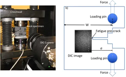
The specimen was a fine grained granitic rock with a surface area of 60 _! 60 mm2 and a thickness of 10 mm. An annotated photo of the test set up is shown in Figure 7a; the sample width was (2W) was 60 mm, each of its notch length (a) was 10, and each of its notch radii (d) was 5 mm. The studied material was a fine-grained granitic rock. To make the texture more prominent in the images, the surface of the specimen was polished in a grinding machine before testing. This allowed the natural pattern of the specimen be used for DIC analysis without need for an artificial speckle pattern (e.g. spray paint) which can obscure the crack tip. However, this method can result in blurriness in the speckle pattern due to the height difference of the surface asperities. Therefore, to evaluate the effectiveness of the natural pattern of the specimen as speckle pattern, a detailed noise analysis was performed which is explained in the next section.

The specimen was glued to the loading platens of the testing machine, ensuring that the loading line and the centre axis of the specimen coincided as close as possible. The tensile load was controlled at a constant crosshead displacement rate of 0.06 mm/min.

A 2D DIC measurement setup comprised a 4 megapixel CCD camera and a Schneieder-Kreuznach Componon-S 2.8/50 Macro lens was used for the image acquisition. The observed area (65 × 65 mm2) covered slightly more than the entire specimen surface, corresponding to a pixel size of approximately 32 µm/pixel. To obtain high contrast levels, the specimen was illuminated by a white LED light panel.

5.1.2_! Analysis and discussion

A sequence of 8 bit 2048x2048 pixel images were obtained (e.g. Figure 8a) as described above, from which a smaller region of 1329x681 pixels was selected (indicated in Figure 8a with a white dashed box) to reduce computation time and to mask the round tip of the notch. The region of interest before and after load (i.e. reference and deformed images, Figure 8b and c) shows two cracks in the deformed image. The PC-based algorithm could be used to detect and analyse multiple cracks, but for simplicity, only the larger surface discontinuity labelled in the figure as “Crack” was considered in this study. A DIC analysis was performed on the images using least square method with subset size 17 and step size of 4; no smoothing or outlier filter was applied. The calculated opening displacement map, Uy, is shown in Figure 8d. To estimate the expected noise within the displacement field, a baseline noise analysis (no deformation / movement) is conducted with the same DIC parameters giving a noise level of σ

Ux =0.009 and σUy =0.012 pixels which is similar to the Medium noise analysis that was

It is observed that the mean grey-level intensity within the region of interest changes from 85.3 to 86.5 counts between reference and deformed images. This change of grey-level intensity can be visually seen at the location of the discontinuity which leads to poor correlation for the subsets that include the crack, as shown by the censored displacement data (Figure 8d). Subsets with correlation coefficient of less than 60% were censored. The missing data were extrapolated using a linear least square approach without modifying known values to obtain the final displacement field (Figure 8e).

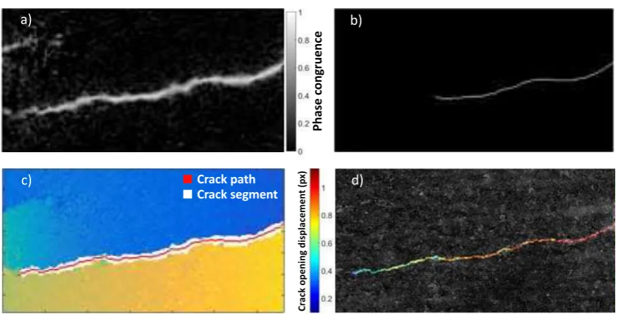
The key steps of the application of the crack detection algorithm are depicted in Figure 9: this shows the outcome of the phase-congruency analysis (Figure 9a), the path segmentation using Hough transform on the phase congruency result (Figure 9b); an overlay of the segmented crack on the displacement data (Figure 9c) and the crack opening profile (Figure 9d) on the deformed image. The algorithm successfully extracted the discontinuity and quantified its length, opening displacement profile and path. Visual inspection of the data shows that the crack path has been identified with an accuracy better than 2 pixels. Close to the crack tip and the COD is less than a pixel accurate.

5.2_! Ductile test

5.2.1_! Experiment details

Ductile materials show high levels of plasticity around the crack and therefore the large strains of the surface can induce errors in the digital image correlation analysis. A fracture test of aluminium alloy 2024 was carried according to ASTM E399 [73], details of which is given elsewhere [74]; a brief description of the experiment is given here. A fatigue precraked Compact Tension (CT) specimen, schematic of the which is shown in Figure 7b, with a width of W=50mm and a/W=0.5 (a is the crack length) was tested; other dimensions of the specimen are related to W according to ASTM E399. The specimen was loaded by moving the upper loading pin at a constant displacement rate of 0.2 mm/min until the crack started growing. The loading of a CT sample is predominantly dominated by bending around a plastic hinge unlike the DENT specimens tested in the previous section which is mainly tensile. This change of loading mode provides an extra degree of dissimilarity between the two experiments in addition to the difference in material behaviour to evaluate the performance of PC algorithm further.

The images were collected using a stereo-DIC system comprising 2 Toshiba-Teli CSB4000CL-10A cameras; each camera captured 2008×2047 pixel size 10-bit images of the surface of the specimen which had a painted speckle pattern applied to it. The pixel size was 15 µm, calibrated using a 058-5 LaVision 3D calibration plate.

5.2.2_! Analysis and discussion

A pair of stereo images, comprising four images, was analysed: two reference images recorded by cameras at different angles to the surface of the undeformed specimen, and two similarly recorded images of the loaded specimen. An example of an image captured by the left camera, after the distortion correction, is shown in Figure 11a. For a faster computational analysis, a region of interest of 400x300 pixels was selected (marked by a dashed white box in Figure 11a). This region of interest is compared in Figure 11b and Figure 11c for the reference and deformed images. The same region, observed by optical microscopy at low magnification, is shown in Figure 11d.

The images were analysed with subset size 9 and step size of 1 to obtain the displacement fields shown in Figure 12a. Increased numbers of missing vectors (shown as white patches to the right side of the displacement map) occurred due a loss of focus during the experiment (see Figure 11b and Figure 11c). However, the non-correlated areas are mostly local, which allowed interpolation to be used results of which is given in Figure 12b. Best user judgement was employed to manually segment the crack, which is shown with a red line with the crack tip identified by a white cross.

The Phase Congruency map of the displacement field, shown in Figure 12c, highlights the discontinuity quite clearly. The crack opening displacement profile, calculated automatically by the algorithm is give in Figure 12d and that of the crack path in Figure 12e. They are overlaid on the images taken during digital image correlation experiment. The crack path was also overlaid on the stitched image taken by the optical microscope with low magnification and is shown in Figure 12f. In these figures, the manual segmentation is represented in red while the automatically identified crack path is given by green. It is appropriate to take the manual segmentation of the crack (red line) as true data as higher resolution of the surface was captured and the crack path calculated. Using Eq. 8, RMS error between manual segmentation and crack path proposed by this study is calculated to be 2.53 pixel over the whole length of the crack. Significantly, the time required to obtain the displacement field and the crack parameters using the proposed algorithm was approximately 1 min 22 seconds including the DIC analysis. The time to map the crack manually by optical microscope was approximately 10 hours.

Ductile materials can experience significant crack tip blunting before crack propagation. PC method identifies the discontinuity in the displacement field accurately, therefore, it is not sensitive to the width of the crack, hence its blunting. However, large scale crack blunting that results in a crack mouth opening displacement reduces the accuracy of digital image correlation considerably. This is because there is no speckle pattern in the empty space created by the crack blunting which reduces the success of the correlation function in matching the speckle patterns. In short, PC is not sensitive to crack blunting but DIC is and therefore care should be taken when applying the method to initiation stage of largely blunt cracks.

6

_!

Concluding remarks

¥! A new phase congruency (PC) based algorithm has been proposed to automatically segment cracks and extract their quantifying parameters such as crack path, length and opening displacement profile.

¥! Applied to materials with different levels of deformation around the crack tip, the difference between manual image segmentation and the faster, autonomous PC-based algorithm is less than three pixels.

References

[1] D. Marr and E. Hildreth, "Theory of edge detection," Proceedings of the Royal Society of London. Series B. Biological Sciences, vol. 207, pp. 187-217, 1980.

[2] P. Dare, H. Hanley, C. Fraser, B. Riedel, and W. Niemeier, "An operational application of automatic feature extraction: the measurement of cracks in concrete structures," The Photogrammetric Record, vol. 17, pp. 453-464, 2002.

[3] I. Abdel-Qader, O. Abudayyeh, and M. E. Kelly, "Analysis of edge-detection techniques for crack identification in bridges," Journal of Computing in Civil Engineering, vol. 17, pp. 255-263, 2003.

[4] T. Yamaguchi and S. Hashimoto, "Fast crack detection method for large-size concrete surface images using percolation-based image processing," Machine Vision and Applications, vol. 21, pp. 797-809, 2010.

[5] S. Roux, J. Réthoré, and F. Hild, "Digital image correlation and fracture: an advanced technique for estimating stress intensity factors of 2D and 3D cracks," Journal of Physics D: Applied Physics, vol. 42, p. 214004, 2009.

[6] S. Avril, A. Vautrin, and Y. Surrel, "Grid method: application to the characterization of cracks," Experimental mechanics, vol. 44, pp. 37-43, 2004.

[7] W. Peters and W. Ranson, "Digital imaging techniques in experimental stress analysis," Optical Engineering, vol. 21, pp. 213427-213427-, 1982.

[8] M. Sutton, W. Wolters, W. Peters, W. Ranson, and S. McNeill, "Determination of displacements using an improved digital correlation method," Image and vision computing, vol. 1, pp. 133-139, 1983.

[9] T. Chu, W. Ranson, and M. Sutton, "Applications of digital-image-correlation techniques to experimental mechanics," Experimental mechanics, vol. 25, pp. 232-244, 1985.

[10] H. W. Schreier and M. A. Sutton, "Systematic errors in digital image correlation due to undermatched subset shape functions," Experimental Mechanics, vol. 42, pp. 303-310, 2002. [11] B. Pan, K. Qian, H. Xie, and A. Asundi, "Two-dimensional digital image correlation for in-plane

displacement and strain measurement: a review," Measurement science and technology, vol. 20, p. 062001, 2009.

[12] B. Pan, A. Asundi, H. Xie, and J. Gao, "Digital image correlation using iterative least squares and pointwise least squares for displacement field and strain field measurements," Optics and Lasers in Engineering, vol. 47, pp. 865-874, 2009.

[13] "Davis 8.2.6 software – Lavision."

[14] S. McNeill, W. Peters, and M. Sutton, "Estimation of stress intensity factor by digital image correlation," Engineering fracture mechanics, vol. 28, pp. 101-112, 1987.

[15] J. Rethore, A. Gravouil, F. Morestin, and A. Combescure, "Estimation of mixed-mode stress intensity factors using digital image correlation and an interaction integral," International Journal of Fracture, vol. 132, pp. 65-79, 2005.

[16] T. Becker, M. Mostafavi, R. Tait, and T. Marrow, "An approach to calculate the J-integral by digital image correlation displacement field measurement," Fatigue & Fracture of Engineering Materials & Structures, vol. 35, pp. 971-984, 2012.

[17] R. Hamam, F. Hild, and S. Roux, "Stress intensity factor gauging by digital image correlation: Application in cyclic fatigue," Strain, vol. 43, pp. 181-192, 2007.

[19] S. Roux and F. Hild, "Stress intensity factor measurements from digital image correlation: post-processing and integrated approaches," International Journal of Fracture, vol. 140, pp. 141-157, 2006.

[20] L. S.-M. S.M. Barhli, M.S.L. Jordan, A.F. Cinar, C. Reinhard, M. Mostafavi, T.J. Marrow, "Synchrotron X-ray Characterisation of Crack Strain Fields in Polygranular Graphite," 2017. [21] J. R. Rice, "A path independent integral and the approximate analysis of strain concentration

by notches and cracks," Journal of applied mechanics, vol. 35, pp. 379-386, 1968.

[22] M. Gosz, J. Dolbow, and B. Moran, "Domain integral formulation for stress intensity factor computation along curved three-dimensional interface cracks," International Journal of Solids and Structures, vol. 35, pp. 1763-1783, 1998.

[23] J. Chen, X. Zhang, N. Zhan, and X. Hu, "Deformation measurement across crack using two-step extended digital image correlation method," Optics and Lasers in Engineering, vol. 48, pp. 1126-1131, 2010.

[24] J. Poissant and F. Barthelat, "A novel “subset splitting” procedure for digital image correlation on discontinuous displacement fields," Experimental mechanics, vol. 50, pp. 353-364, 2010. [25] W. Elber, "The significance of fatigue crack closure," in Damage tolerance in aircraft

structures, ed: ASTM International, 1971.

[26] R. J. Donahue, H. M. Clark, P. Atanmo, R. Kumble, and A. J. McEvily, "Crack opening displacement and the rate of fatigue crack growth," International Journal of Fracture Mechanics, vol. 8, pp. 209-219, 1972.

[27] W. Yisheng and J. Schijve, "Fatigue crack closure measurements On 2024-T3 sheet specimens," Fatigue & Fracture of Engineering Materials & Structures, vol. 18, pp. 917-921, 1995.

[28] N. Walker and C. Beevers, "A fatigue crack closure mechanism in titanium," Fatigue & Fracture of Engineering Materials & Structures, vol. 1, pp. 135-148, 1979.

[29] M. A. Sutton, M. L. Boone, F. Ma, and J. D. Helm, "A combined modeling–experimental study of the crack opening displacement fracture criterion for characterization of stable crack growth under mixed mode I/II loading in thin sheet materials," Engineering Fracture Mechanics, vol. 66, pp. 171-185, 2000.

[30] J. D. Helm, "Digital image correlation for specimens with multiple growing cracks," Experimental mechanics, vol. 48, pp. 753-762, 2008.

[31] P. Lopez-Crespo, A. Shterenlikht, E. Patterson, J. Yates, and P. Withers, "The stress intensity of mixed mode cracks determined by digital image correlation," The Journal of Strain Analysis for Engineering Design, vol. 43, pp. 769-780, 2008.

[32] J. Réthoré, F. Hild, and S. Roux, "Extended digital image correlation with crack shape optimization," International Journal for Numerical Methods in Engineering, vol. 73, pp. 248-272, 2008.

[33] E. Fagerholt, T. Børvik, and O. Hopperstad, "Measuring discontinuous displacement fields in cracked specimens using digital image correlation with mesh adaptation and crack-path optimization," Optics and Lasers in Engineering, vol. 51, pp. 299-310, 2013.

[34] T. L. Nguyen, S. A. Hall, P. Vacher, and G. Viggiani, "Fracture mechanisms in soft rock: Identification and quantification of evolving displacement discontinuities by extended digital image correlation," Tectonophysics, vol. 503, pp. 117-128, 4/25/ 2011.

[35] C. Eberl, D. Gianola, and K. Hemker, "Mechanical characterization of coatings using microbeam bending and digital image correlation techniques," Experimental mechanics, vol. 50, pp. 85-97, 2010.

[36] W. Mekky and P. S. Nicholson, "The fracture toughness of Ni/Al 2 O 3 laminates by digital image correlation I: experimental crack opening displacement and R-curves," Engineering fracture mechanics, vol. 73, pp. 571-582, 2006.

[38] J. Carroll, C. Efstathiou, J. Lambros, H. Sehitoglu, B. Hauber, S. Spottswood, et al., "Investigation of fatigue crack closure using multiscale image correlation experiments," Engineering Fracture Mechanics, vol. 76, pp. 2384-2398, 2009.

[39] S. Alam, A. Loukili, and F. Grondin, "Monitoring size effect on crack opening in concrete by digital image correlation," European journal of environmental and civil engineering, vol. 16, pp. 818-836, 2012.

[40] Q. Lin and J. F. Labuz, "Fracture of sandstone characterized by digital image correlation," International Journal of Rock Mechanics and Mining Sciences, vol. 60, pp. 235-245, 2013. [41] J. Duff and T. Marrow, "In situ observation of short fatigue crack propagation in oxygenated

water at elevated temperature and pressure," Corrosion Science, vol. 68, pp. 34-43, 2013. [42] M. Mostafavi, S. McDonald, H. Çetinel, P. Mummery, and T. Marrow, "Flexural strength and

defect behaviour of polygranular graphite under different states of stress," Carbon, vol. 59, pp. 325-336, 2013.

[43] L. Babout, T. Marrow, D. Engelberg, and P. Withers, "X-ray microtomographic observation of intergranular stress corrosion cracking in sensitised austenitic stainless steel," Materials Science and Technology, vol. 22, pp. 1068-1075, 2006.

[44] M. Williams, "The bending stress distribution at the base of a stationary crack," Journal of applied mechanics, vol. 28, pp. 78-82, 1961.

[45] S. Vanlanduit, J. Vanherzeele, R. Longo, and P. Guillaume, "A digital image correlation method for fatigue test experiments," Optics and Lasers in Engineering, vol. 47, pp. 371-378, 2009. [46] P. Kovesi, "Phase congruency: A low-level image invariant," Psychological research, vol. 64,

pp. 136-148, 2000.

[47] P. Kovesi, "Phase congruency detects corners and edges," in The australian pattern recognition society conference: DICTA 2003, 2003.

[48] M. C. Morrone and D. Burr, "Feature detection in human vision: A phase-dependent energy model," Proceedings of the Royal Society of London B: Biological Sciences, vol. 235, pp. 221-245, 1988.

[49] M. C. Morrone, J. Ross, D. C. Burr, and R. Owens, "Mach bands are phase dependent," Nature, vol. 324, pp. 250-253, 1986.

[50] M. C. Morrone and R. A. Owens, "Feature detection from local energy," Pattern recognition letters, vol. 6, pp. 303-313, 1987.

[51] M. C. Morrone and D. Burr, "Feature detection in human vision: A phase-dependent energy model," Proceedings of the Royal Society of London. Series B, biological sciences, pp. 221-245, 1988.

[52] S. Venkatesh and R. Owens, "On the classification of image features," Pattern Recognition Letters, vol. 11, pp. 339-349, 1990.

[53] P. Kovesi, "Phase congruency mono algorithm MATLAB CODE," 2013.

[54] W. Lijuan, Z. Changsheng, L. Ziyu, S. Bin, and T. Haiyong, "Image feature detection based on phase congruency by Monogenic filters," in Control and Decision Conference (2014 CCDC), The 26th Chinese, 2014, pp. 2033-2038.

[55] M. Kass, A. Witkin, and D. Terzopoulos, "Snakes: Active contour models," International journal of computer vision, vol. 1, pp. 321-331, 1988.

[56] H. Fang, J. Kim, and J.-W. Jang, "A Fast Snake Algorithm for Tracking Multiple Objects," JIPS, vol. 7, pp. 519-530, 2011.

[57] S. Lankton, D. Nain, A. Yezzi, and A. Tannenbaum, "Hybrid geodesic region-based curve evolutions for image segmentation," in Medical Imaging, 2007, pp. 65104U-65104U-10. [58] D. Lanman, "Bilateral Filtering, MATLAB Central File Exchange," 2006.

[59] B. Zhang and J. P. Allebach, "Adaptive bilateral filter for sharpness enhancement and noise removal," Image Processing, IEEE Transactions on, vol. 17, pp. 664-678, 2008.

[61] D. H. Ballard, "Generalizing the Hough transform to detect arbitrary shapes," Pattern recognition, vol. 13, pp. 111-122, 1981.

[62] J.-S. Lee, "Digital image smoothing and the sigma filter," Computer Vision, Graphics, and Image Processing, vol. 24, pp. 255-269, 1983.

[63] P. J. G. Schreurs, "Fracture Mechanics " Eindhoven University of Technology, 2012.

[64] D. Smith, M. Ayatollahi, and M. Pavier, "The role of T-stress in brittle fracture for linear elastic materials under mixed-mode loading," Fatigue & Fracture of Engineering Materials & Structures, vol. 24, pp. 137-150, 2001.

[65] "Edge Detector 1D (Gaussian Kernel 1D) ,

http://cismm.web.unc.edu/resources/tutorials/edge-detector-1d-tutorial/."

[66] S. Barhli, D. Hollis, B. Wieneke, M. Mostafavi, and T. Marrow, "Advanced 2D and 3D Digital Image Correlation of the Full-Field Displacements of Cracks and Defects," in Evaluation of Existing and New Sensor Technologies for Fatigue, Fracture and Mechanical Testing, ed: ASTM International, 2015.

[67] J. C. Mullikin, L. J. van Vliet, H. Netten, F. R. Boddeke, G. van der Feltz, and I. T. Young, "Methods for CCD camera characterization," 1994, pp. 73-84.

[68] S. A. Stanier, J. Blaber, W. A. Take, and D. White, "Improved image-based deformation measurement for geotechnical applications," Canadian Geotechnical Journal, vol. 53, pp. 727-739, 2015.

[69] A. Baldi and F. Bertolino, "Experimental analysis of the errors due to polynomial interpolation in digital image correlation," Strain, vol. 51, pp. 248-263, 2015.

[70] W. Tong, "Subpixel image registration with reduced bias," Optics letters, vol. 36, pp. 763-765, 2011.

[71] A. Sousa, J. Xavier, M. Vaz, J. Morais, and V. Filipe, "Cross-Correlation and Differential Technique Combination to Determine Displacement Fields," Strain, vol. 47, pp. 87-98, 2011. [72] J. Franklin, S. ZONGQI, B. Atkinson, P. Meredith, F. Rummel, W. Mueller, et al., "Suggested

methods for determining the fracture toughness of rock," INTERNATIONAL JOURNAL OF ROCK MECHANICS AND MINING & GEOMECHANICS ABSTRACTS, vol. 25, 1988.

[73] E. Astm, "399-90:" Standard test method for plane-strain fracture toughness of metallic materials," Annual book of ASTM standards, vol. 3, pp. 506-536, 1991.

Appendix A: Mathematical representation of phase congruency

PC(x) – value of pixel x in an image is computed by:

&' " = N M^N " _MN " ∆ΦMN " − aN

_MN " + b

M N

(A-1)

where o and n denote the indexes over orientation and wavelet scale respectively. The function ∗ returns its enclosed quantity when the value is positive and zero otherwise. ^ is a weighting factor based on frequency spread and ∆Φ(x) is a measure of phase congruency.

On a given orientation and a fixed number of wavelet scale, a value for amplitude, _, is estimated by designing a filter bank considering both radial and angular components. The radial component of the filter bank is designed in terms of log-Gabor function. On a linear

frequency scale the log-Gabor function is defined as e_f = g

hijk l m n

nopq r n _{where - is the radius}

filter given in pixels in the polar system and , controls the filter bandwidth. The function s is calculated by s = t

uvwx

where y_ZV[ = y_ZOM. zMWt. z is the scaling between the centre

frequencies of successive filters and n is the number of wavelet scales. The angular

component of the filter bank is calculated by '{ = g

h(|h|})n

nr|n _{where .O =} OWt ~

N , K indicates the

current orientation and  is the number of orientation. ,_{ = ~

Ä.N where Å is the ratio of

angular interval between filter orientations and standard deviation of the angular Gaussian function.

On a given orientation, the weighting function, ^ " , and measure of phase congruency,

∆Φ(x), are calculated as following:

^ " = 1

1 + gÇ(ÉWP [ ) (A-2)

where “Ñ” is a cut-off value of filter, Ö is the gain factor that controls the sharpness of the cut-off and

Ü " = t

F

áà [ à

âäávwx [

where J is the total number of scales being considered. b = 0.001 is

added to prevent division of zero in numerical calculation. For a given wavelet scale, ã, a measure for phase congruency is calculated as following:

∆Φ x = cos åM " − å " − sin åM " − å " (A-3)

where å_M " is the local phase of the amplitude __M " and the value of å " that maximizes

_MN " ∆ΦMN " is the amplitude weighted mean local phase angle of all the Fourier terms at

Appendix B: Heaviside step function

The Heaviside step function can be used to fit a discontinuous function to the displacement field line profile normal to the crack for every profile along the crack. This is usually used to obtain the crack opening displacement. The Heaviside step function is defined as;

ç " =

0 " < 0

1/2 " = 0

1 " > 0

(B-1)

However, the discontinuity location or crack path is needed before fitting the Heaviside function to the line profile. Three different methods have been looked at to find the crack location:

¥! Global maximum gradient of the line profile across the discontinuity

¥! Maximum of difference between windowed moving average with a set smoothing threshold

¥! 1D canny edge detector - Convolution with a Gaussian derivative kernel with a selected noise suppression [65]

Appendix C: Spatial resolution analysis

Digital image correlation analysis by least square method requires a step size and a subset size (TPëíPQì), which are selected by the user. The subset size is the area over which the

averaged displacement measurement is calculated and the step size (TPìQî) represents the

distance between each subset, and so affects the overlap. This overlapping of subsets increases the spatial resolution of the displacement field, and also acts to smooth it. This can have a significant effect if the displacement gradient is steep. The percentage overlap is defined by:

ïAg-ñ1ó % =TPëíPQì− TPìQî

TPëíPQì

(C-1)

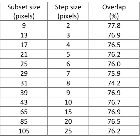
The effect of the subset size on the accuracy of the crack parameters calculated by the PC-based algorithm was investigated using sets of DIC parameters chosen to achieve a constant overlap for direct comparison of data.

Table 1 least square DIC parameters used for Spatial resolution study

Subset size (pixels)

Step size (pixels)

Overlap (%)

9 2 77.8

13 3 76.9

17 4 76.5

21 5 76.2

25 6 76.0

29 7 75.9

31 8 74.2

39 9 76.9

43 10 76.7

65 15 76.9

85 20 76.5

105 25 76.2

The study was performed on the virtual experiment with CMOD = 1 px, with no noise added. This was chosen as the crack is not visible on the deformed image, so the analysis is unaffected by subsets overlapping the open crack. The obtained COD, crack length and crack path were compared to the synthetic crack parameters used to deform the initial image.

Increasing the subset size (Figure C-a) smooths the displacement field and the COD values are more precise, but this results in a loss in spatial resolution and hence loss of accuracy in the detected crack path. Decreasing the subset size increases the spatial resolution, which better defines the crack path to enable crack detection to carried out more accurately (see Figure C-b and Figure C-c). Although it is expected that the relation C-between suC-bset size and error would be linear, outliers in Figure C-b and Figure C-c can be identified. This is due to the inconsistent data point positioning for each spatial resolution analysis. It is therefore can be concluded that the data point positioning plays a significant role in the accurate calculation of the crack feature.

Figures

Figure 1- (a) a 2024x2048 pixel synthetic image containing a crack with mouth opening displacement of 1 pixel; b) An image similar to (a) with crack mouth opening displacement of 5 pixels; (c) Opening (i.e., direction) displacement of associated with image (a) d) Opening (i.e.,

Y-direction) displacement associated with image (b) e) Opening strain of (c) f) Opening strain of (d)

Figure 2 - (a) Normalized theoretical displacement field associated with a cracked plate (b) Normalized strain map of (a) c) Phase congruency of (b) (d) Vertical line profile across the crack mouth, one in every ten data point are shown e) Vertical line profile across the crack tip, one in

Figure 3 - PC-based crack detection algorithm flowchart

Figure 4 - Noise analysis (a) error analysis for Crack opening displacement (b) error analysis for crack path (c) relative crack length error with different additive noise

Figure 5 - Image noise analysis (a) image noise vs signal to noise ratio and displacement standard deviation error b) image noise vs missing data

Figure 6 - Analysis of crack detection methods (a) Uy map associated with a crack opening

displacement of 0.1 pixels with high additive image noise (b) crack opening displacement error (c) crack path error (d) crack length error

a) b)

O

p

e

n

in

g

d

isp

la

ce

m

e

n

t,

Uy

(mm)

a) b)

Figure 7 - (a) the small scale doubled edge notch tensile test setup of quasi-brittle material: 2W (width) =60 mm, a (notch length) =10 mm, and d (notch radius) = 5 mm (b) Fracture test of ductile

material

Figure 8 - Quasi-Brittle test and analysis (a) captured image of the surface, region of interest is indicated between two white dashed lines (b) reference region of interest (c) deformed region of interest d) calculated opening dispalcment Uy field (e) extrapolated Uy displacement field with no

missing data points Rock specimen

Crosshead

DIC Camera

Force

Force Loading pin Loading pin

W

DIC image

Fatigue pre-crack

a) _b)

!

Deformed Image

Crack Reference Image

a) _{b) c)}

d)

2048 px

2

0

4

8

p

x

1329 px

6

8

1

p

x

x

y _{100 px}

U

y

d

is

p

la

ce

m

e

n

t

fi

e

ld

(

p

x

)

Figure 9 - PC-based crack detection (a) phase congruency of Figure 8e (b) segmentation using Hugh transformation (c) segmented crack path overlaid on the displacement field (d) Crack path and

crack opening displacement profile overlaid on the deformed image

Figure 10 - Optical microscopy analysis (a) lower magnification image (b) higher magnification image (c) high and Low magnification image stitched (d) zoomed in of (c)

Figure 11 - Ductile fracture test and analysis (a) full field reference image from left-hand camera (b) region of interest reference image (c) region of interest deformed image (d) stitched image of

optical microscopy (see Figure 10c) of the same region as shown in (b) d)

b)

c) Crack path

Crack segment a) P h a se c o n g ru e n ce C ra ck o p e n in g d is p la ce m e n t (p x ) 10000 px a) b) Crack tip c) d) 1.4 mm 1000 px 1.04mm 1000 px 1.04mm a) 400 px 300 px x

y 100 px

Figure 12 - Stereo-DIC analysis (a) Uy map (b) missing Uy map extrapolated (c) Phase Congruency of Uy map (d) crack opening displacement (e) crack path calculated by the algorithm (f) crack path

calculated by the algorithm

Figure C - Spatial Resolution study to show the effect of subset size on the root mean square error of (a) crack opening displacement (b) crack path and (c) crack length

a)

a) b) c)

f)

d) e)

0 100 200 300 400 Uydisplacement field (pixel)

Micro – Crack tip Micro – Crack path PC – Crack path