On the orthogonalised reverse path method for nonlinear system identification

promoting access to White Rose research papers

Universities of Leeds, Sheffield and York

http://eprints.whiterose.ac.uk/

This is an author produced version of a paper published in Journal of Sound and Vibration.

White Rose Research Online URL for this paper:

Published paper

Muhamad, P., Sims, N., Worden, K. (2012) On the orthogonalised reverse path method for nonlinear system identification, Journal of Sound and Vibration, 331 (20), pp. 4488-4503

ON THE ORTHOGONALISED REVERSE PATH METHOD

FOR NONLINEAR SYSTEM IDENTIFICATION

P. Muhamad, N.D. Sims and K. Worden1

Dynamics Research Group, Department of Mechanical Engineering,

University of Sheffield, Mappin Street, Sheffield S1 3JD,UK.

Abstract. The problem of obtaining the underlying linear dynamic compliance matrix in the presence of nonlinearities in a general Multi-Degree-of-Freedom (MDOF) system can be solved using the Conditioned Reverse Path (CRP) method introduced by Richards and Singh (1998 Journal of Sound and Vibration, 213(4): p. 673-708). The CRP method also provides a means of identifying the coefficients of any nonlinear terms which can be specified a priori in the candidate equations of motion. Although the CRP has proved extremely useful in the context of nonlinear system identification, it has a number of small issues associated with it. One of these issues is the fact that the nonlinear coefficients are actually returned in the form of spectra which need to be averaged over frequency in order to generate parameter estimates. The parameter spectra are typically polluted by artefacts from the identification of the underlying linear system which manifest themselves at the resonance and anti-resonance frequencies. A further problem is associated with the fact that the parameter estimates are extracted in a recursive fashion which leads to an accumulation of errors. The first minor objective of this paper is to suggest ways to alleviate these problems without major modification to the algorithm. The results are demonstrated on numerically-simulated responses from MDOF systems. In the second part of the paper, a more radical suggestion is made, to replace the conditioned spectral analysis (which is the basis of the CRP method) with an alternative time domain decorrelation method. The suggested approach – the Orthogonalised Reverse Path (ORP) method – is illustrated here using data from simulated Single-Degree-of-Freedom (SDOF) and MDOF systems.

1.

Introduction

The discussion of system identification methods for nonlinear structural systems typically

starts with Single Degree-of-Freedom (SDOF) systems. The groundbreaking work of Duffing

[1], demonstrated in the earliest stages of research how easily nonlinearities can be produced,

and the significant effect that they have on system response for a SDOF oscillator with a

cubic stiffness. Since Duffing’s work, many techniques have been developed which seek to

indicate the presence of nonlinearity in a given system and to estimate the extent of any

nonlinear contributions. The methods include: by-passing the nonlinearity by linearisation,

time and frequency domain methods, modal methods, time-frequency analysis, black-box

modelling and structural model updating; a fairly recent and comprehensive and review can

be found in [2].

The conventional identification method for linear systems using time or frequency domain

data is the modal parameter estimation technique [3]. The frequency domain technique

extracts modal parameters from the and Frequency Response Functions (FRFs)2

;

however, if the system under identification also possesses nonlinearities or is subject to

correlated noise, these conventional estimates often yield biased FRFs from which accurate

model parameters cannot be determined [4]. Standard spectral methods are also incapable of

identifying the nonlinearities. The most often used identification method for general linear

MDOF systems, using input and output response measurements is based on modal analysis

[5].

The modal method uses an assumption of orthogonality of the normal modes of the system

and the subsequent decoupling of the equations of motion by using the modal vector.

Unfortunately, where there is significant modal coupling through non-proportional damping

or nonlinear interaction, the approach can become unsatisfactory [6]. Extended frequency

domain methods for nonlinear systems have been proposed in the literature; among them are

the Volterra and Wiener series [7]; however when these methods are implemented for MDOF

systems they are typically cumbersome to compute and interpret, and the difficulty increases

dramatically with higher-order approximations [8]. Higher-order spectra have also received

1

some consideration for system identification and have the capability to detect the presence of

the nonlinearity and provide some qualitative information about the nonlinear behaviour,

such as the type of nonlinearity [9]. The Nonlinear Identification through Feedback of the

Outputs (NIFO) method [10] is a recent spectral approach for identification of MDOF

nonlinear systems; it can be used to eliminate the distortions caused by the presence of

nonlinearities in FRFs. The correlation between the linear and nonlinear terms may be an

issue and care must be taken to achieve a good conditioning of the data matrices.

From the many recent methods listed in [2], an approach for identifying MDOF nonlinear

systems which is based on the Reverse Path (RP) formulation is selected for consideration here. The RP method was originally introduced as a spectral method by Bendat in [11]; it

involves mathematically reversing the input-to-output path for the given dynamical system,

then applying traditional spectral techniques for analysis. The method is a frequency domain

one because the data considered during the identification process take the form of FRFs or

spectra; the method offers easy computation and has an intuitive interpretation. The original

RP method aimed to identify nonlinear structures, but Bendat’s approach worked for only

SDOF systems. Since Bendat’s early work, the RP technique has been generalised to MDOF

systems by Rice and Fitzpatrick [8] and Richards and Singh [12]. The first method required

that excitations be applied at every response location; however, in practice the number of

excitations is always smaller than the number of measured responses. This drawback was

addressed by the introduction of the Conditioned Reverse Path method (CRP) in [12]. There

are several works where the CRP method has been applied to numerical models [13] and real

nonlinear systems [14-15]. The authors of the latter works generally agreed that the CRP

method is capable of detecting and quantifying nonlinearities in MDOF systems excited by

random noise.

In Sections 2-4 of the present paper some minor issues with the CRP method are

highlighted; one of these is the fact that the coefficients of nonlinear terms in the model are

expressed as spectra (functions of frequency) and are converted to the required scalars by

computing the spectral mean. Whilst this spectral estimate could be advantageous for the

identification of certain nonlinearities (e.g. viscoelastic effects), the parameter spectra are

typically polluted by artefacts from the identification of the underlying linear system which

2

manifest themselves at the resonance and antiresonance frequencies. A further problem is that

the parameter estimates are extracted in a recursive fashion which accumulates errors. The

present contribution suggests two simple ways to alleviate these problems without major

modification to the algorithm.

Despite its obvious usefulness and established record, one arguable drawback of the CRP

method has actually proved to be its dependence on the conditioned spectral analysis, which is

a comparatively complicated approach to the decorrelation of spectra. With this in mind, the

second and main objective of the current paper is to suggest an alternative time domain

approach, referred to as the Orthogonalised Reverse Path (ORP) method. The ORP method is

able to decorrelate the initial time data and remove the effects of nonlinearity before passing

to the frequency domain, hopefully giving unbiased estimates of the FRF and compliance

matrices. The approach provides an extremely simple formulation for the problem of

characterising the underlying linear dynamics and may well also lead to simplifications in the

estimation of coefficients of nonlinear terms. The basic theory of the proposed approach is

given in Section 5 of the present manuscript, and the performance is illustrated using

numerical examples in Section 6.

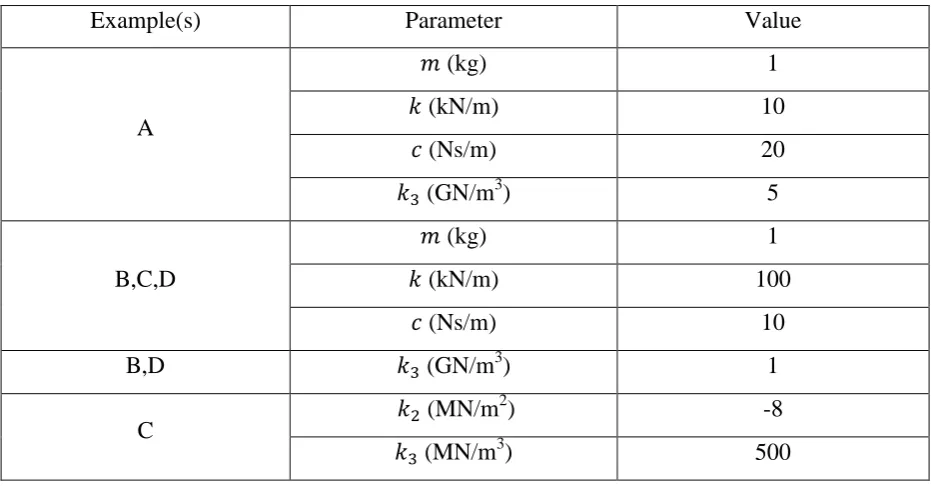
Throughout this manuscript, four numerical examples are used to illustrate and compare

the performance of the proposed methods. At this stage it is useful to briefly introduce these

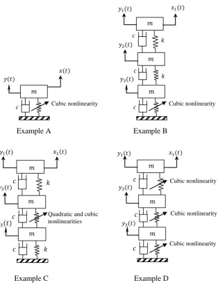
example systems. With reference to Figure 1, Example A is a classical SDOF Duffing

oscillator. Example B is a 3-DOF system with a single cubic nonlinear stiffness. Example C

also possesses one nonlinear spring, but in this case there is both quadratic and cubic

nonlinearity. Example D involves 3 nonlinear springs, all with identical cubic nonlinearities.

Example A was chosen for its (obvious) simplicity, whilst examples C and D replicate two

scenarios from [12]. The numerical values of the various system parameters are given in

Example(s) Parameter Value

A

(kg) 1

(kN/m) 10

(Ns/m) 20

(GN/m3) 5

B,C,D

(kg) 1

(kN/m) 100

(Ns/m) 10

B,D (GN/m3) 1

C

(MN/m2) -8

(MN/m3) 500

Table 1: Linear and nonlinear parameters for the example systems shown in Figure 1.

2.

Basic Concepts of the CRP Method

There are essentially two steps in the implementation of the CRP algorithm. In the first

step, measured force and response data are used to compute estimates of conditioned spectra which are essentially spectra from which the effects of any nonlinearities have been removed.

The conditioned spectra are basically those of the underlying linear system. In the second step

of the CRP process, the coefficients of any nonlinear terms are estimated using the

conditioned spectra. Each of these steps is prone to errors, and these will be illustrated with

some numerical examples in Section 3. First, the background to the CRP method is presented.

In the original formulation of the CRP method, the equations of motion of the system of

interest were expressed as,

(1)

which incorporates the standard mass, stiffness and damping matrices (throughout this paper,

which encodes the nonlinear functions or restoring forces. It is useful to have a

priori knowledge of the locations and types of the nonlinearities present but if these are uncertain, additional functions may be included to capture all possible behaviours, at the cost

of extra computation [12]; a successful identification will yield non-zero coefficients for

significant terms in the expansion and insignificant terms will have coefficients equal or close

to zero.

Taking the Fourier transform of equation (1) yields,

(2)

where is the linear dynamic stiffness matrix. (Throughout this paper frequency

domain objects are denoted by capitals as is standard.)

As discussed above, the CRP is a method based on spectra; following [12], the notation for spectra used here will be as follows: a given spectral matrix is computed by,

(3)

where is the duration of the time segment for the FFT and E is the expectation operator. With reference to (1) and (3), the indices p and q will be taken from the set with

denoting one of the nonlinear functions or spectra . The superscript T

indicates the transpose.

Given the spectra, Frequency Response Functions (FRFs) are calculated from the standard

formulae for spectral estimators [4],

(4)

where and are the autospectral matrices of the input and output vectors

respectively. and are the cross-spectral matrices. The spectra may be conditioned

In the CRP method conditioned spectra are estimated that have had the effects of the

nonlinearities sequentially removed from them as will be explained shortly. If a spectrum has

been conditioned by the removal of the influences of the first r nonlinearities it will be denoted by ; a fully-conditioned spectrum ( ) will simply be denoted by .

Once the conditioning process is complete, the linear FRF matrices can be estimated by,

(5)

where the dagger denotes a pseudo-inverse. In the original CRP paper [12], the coefficients of

nonlinear terms are then estimated through a recursive formula,

(6)

There is a subtlety in the use of this equation which is not made explicit in [12]; it requires

an adjustment to the form,

The calculation begins with the computation of and works backwards to It is clear

from equation (7), that the calculation of the coefficients is very dependent on the accuracy of

the conditioned FRF estimate, and also that there are opportunities for errors to accumulate in

the recursive process. A simple suggestion is made in Section 4 to alleviate the accumulation

problem which is to treat each coefficient in turn as the first term in the 'recursion'.

Application to Example C

The presence of the matrix is best explained by considering the application of the

method to a particular example. For the case of Example C (Figure 1), in terms of equation (2)

one has,

(8)

(9)

By applying the CRP method, one can calculate (elements of) the FRF matrix using

the conditioned estimators as in equations (5a-b). For Example C here, the influence of the

two nonlinear terms are removed. As discussed in [12], only the first column of the FRF

matrix can be obtained if a single excitation is used; however, the matrix can then be

augmented by assuming reciprocity for the underlying linear system and this proves critical in

estimating the coefficients of the nonlinear terms as explained clearly in [12].

In the case of Example C, use of equation (7) finally yields the parameter (spectra)

estimates,

(10)

(11)

It is actually more convenient to work with a slightly modified representation of the system

than equation (2), one takes,

This formulation is simpler to work with but less flexible about grouping nonlinearities.

Using this form, one can explain the origin of the matrix discussed earlier. If one

transposes equation (12), premultiplies by and takes expectations, one obtains,

(13)

(As all spectra in this calculation are conditioned to the same extent, the conditioning indices

will be omitted for the moment.) Pre-multiplying by and post-multiplying by

(which equals by reciprocity) gives,

(14)

Now, extracting the first term from the summation and rearranging a little, one arrives at a

version of the recursion (7),

(15)

where rather than the identity matrix as implied by the original treatment in

[12]. In fact for Example C here,

(16)

from which it can be seen that encodes the location of the nonlinearity, and could be

obtained by inspection. To summarise this example, it can be seen now that the nonlinear

form of equation (7). In the following section this approach is illustrated through the analysis

of three numerical case studies.

3.

Numerical Case Studies for CRP Analysis

With reference to Figure 1, numerical case studies will now be considered based upon

Examples B-D. The responses are simulated by integrating the relevant equations of motion

using a 4th-order Runge-Kutta scheme implemented in Simulink and Matlab. The time step

used for the simulations was 0.0005 seconds throughout. A Gaussian random excitation force

with zero mean and variance 500 N was applied to the first mass in all of the examples.

It is also necessary to specify the relevant signal processing parameters used in the

computation of the spectra and FRFs; once again, these followed [12] so that a comparison

with the results therein was possible. In all cases, 163840 points were generated in total; the

spectra were calculated by dividing the data into 20 non-overlapping segments and averaging.

A Hanning window was used to reduce the affects of leakage.

The case studies of examples C and D will first be used as illustrations to suggest some

minor changes to the CRP algorithm. The CRP algorithm itself was implemented in Matlab

(flow diagrams for the CRP method that explain the various stages in the analysis can be

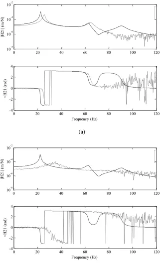
found in [12]). For reference purposes, the unconditioned estimates of the FRFs were

computed. Figure 2 shows the unconditioned estimated compared to the theoretical FRF

from the underlying linear system; the bias which results from the presence of the

nonlinearities is evident; the third resonance for the system is lost completely. (Note that the

three resonance frequencies for the underlying linear system are 22, 63 and 91 Hz

respectively.) .

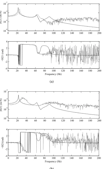
The first stage of the process is to estimate the conditioned FRF estimates as explained in

[12]. (It was found here, as in [12], that the estimator usually proved best, so this was used

for all conditioned estimates. For unconditioned estimates, the bias induced by the

nonlinearity is generally so severe that it does not matter which estimator is used.) As shown

in Figure 3, it is clear that the CRP estimates recover the missing third mode and in fact, a

The final stage of the CRP process is to estimate the coefficients of the nonlinear terms;

equations (10) and (11) are used directly for Example C and appropriate analogues are used

for Example D. As discussed above, the coefficients are first estimated as spectra and then

averaged over frequency to give a scalar parameter estimate. For Example C, the true values

of the parameters are 500 MN/m3 and -8 MN/m2; for Example D,

1 GN/m3. In the case of Example C, the parameter estimates were found to be 554 + 46i

MN/m3 and -7.76 -2.41i MN/m2. The estimates are influenced by fluctuations in the spectra at higher frequencies, but also by artefacts in the spectra which appear to occur at the natural

frequencies (Figure 4), which are probably due to inaccuracies in the linear FRFs from the

conditioned spectral analysis. If a system is forced by a random excitation, one expects to see

fluctuations in the FRF as the Fourier transform of a random time signal is itself a random

variable. Although such fluctuations can sometimes be alleviated by averaging of spectra, in

many cases there will not be enough data to ensure their complete removal. The presence of

the imaginary term is disturbing, but is a result of the estimation procedure of averaging a

complex spectrum; it cannot be regarded as physical in the cases presented here.

The coefficient estimates for Example D were

and . The inaccuracies are again because of artefacts in the spectra. The

results given here are definitely worse than those in the original [12]; the reasons for this are

not completely clear as an attempt was made to adhere to the same FRF estimation strategy

and parameters. There are differences between the coefficient spectra in [12] and here in that

the results here show the presence of more marked artefacts near the modes and this suggests

that the conditioned spectral estimates are the culprit as mentioned for Example C. One reason

for this may be the fact that a fixed-step Runge-Kutta scheme was used here rather than the

adaptive and higher-order algorithm used in [12]. Although this may sound unlikely, the

authors of [12] observed that they obtained improved estimates using the conditioned

rather than the estimator and remarked that this was strange as the data contained no

measurement noise. Their tentative explanation at the time was that this may have been the

result of inaccuracies in the simulation. If this were the case, it is likely that the less

sophisticated simulation scheme used here could well have an effect on the results. Rather

than investigate by resimulating the data, the approach taken here has been to accept that the

current paper is still able to make a principled comparison between methods as all of them are

based on the same simulated time data. Whatever the reason may be for the inferior initial

these arguably would not be necessary when estimates as good as those in [12] are obtained,

they are presented here in the spirit that improvements however minor are desirable and may

be needed if data are from experiment and are therefore subject to measurement noise.

4.

Simple Strategies for Improving Parameter Estimates in CRP

Analysis

The previously estimated coefficient spectra contain significant distortions in the range 20

Hz to 100 Hz and statistical fluctuations at higher frequencies, and this leads to clear bias in

the parameter estimates. One strategy for improving the parameter estimates would be to try

and weight out the distorted regions from the spectra average. Distortions appear at the natural

frequencies of the underlying linear system (and for driving-point FRFs at the

anti-resonances). As observed above, the other source of bias – the fluctuations at higher

frequencies - can be dealt with by placing an upper bound on the frequencies for averaging.

For the purposes of the examples here, only the first 2000 points of the spectra, corresponding

to frequencies below 500 Hz, were used. To pursue now the idea of weighted estimation, a

weighting function is required which has low values at the natural frequencies; the

spectral average can then be computed from,

(17)

An immediate candidate for the weighting function presents itself. The FRF has maxima at

the resonance frequencies and if the conditioned FRF estimate is used, these will be close to

the natural frequencies; this suggests Even so, there are three possible FRFs

for use: receptance, mobility and inertance differing in their low and high-frequency

behaviour. Sadly this first idea for a weighting scheme proved almost completely ineffective;

However, a second candidate for a weighting function quickly suggests itself. If one considers

Figure 4 (or indeed any of the estimated coefficient spectra), it is clear that the distortions in

the imaginary part of the spectrum occur in the same places as in the real part - as one would

measure of the distortion or deviation from constancy. A weighting function can therefore be

constructed by taking the inverse magnitude of the imaginary part. The results of using such a

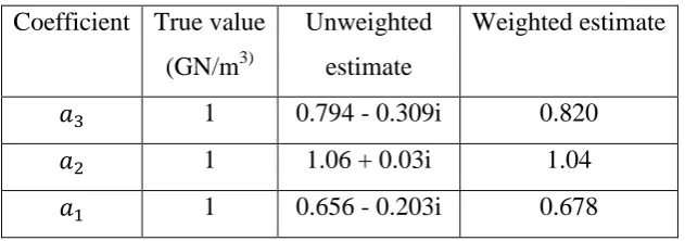
weighting on the parameter estimation process for examples C and D are given in Tables 2

and 3 respectively.

Coefficient True value Unweighted

estimate

Weighted estimate

500 MN/m3 486 + 17i 501.6

-8 MN/m2 -7.65 - 3.35i -7.65

Table 2. Estimated coefficients of nonlinear stiffness terms for Example C (listed in order

of recursive calculation). The weighting function is the inverse magnitude of the imaginary

part of the spectra.

Coefficient True value

(GN/m3)

Unweighted

estimate

Weighted estimate

1 0.794 - 0.309i 0.820

1 1.06 + 0.03i 1.04

1 0.656 - 0.203i 0.678

Table 3. Estimated coefficients of nonlinear stiffness terms for Example D (listed in order

of recursive calculation). The weighting function is the inverse magnitude of the imaginary

part of the spectra.

The use of the imaginary-part weighting produces systematic improvements in the

parameter estimates, although the improvements are very small for Example D.

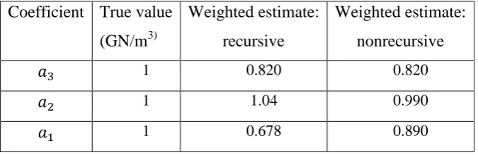
Finally, it has already been observed in a previous section that there is likely to be an

accumulation of errors as a result of using the recursion (7) in order to estimate the spectra for

the coefficients of the nonlinear terms. However, as there is no natural ordering to the

further steps would be superfluous) and thus avoid any cumulative effects of the errors. The

results of using nonrecursive parameter estimates for examples C and D are summarised in

Tables 4 and 5 respectively.

Coefficient True value Weighted estimate:

recursive

Weighted estimate:

nonrecursive

500 MN/m3 501.6 501.6

-8 MN/m2 -7.65 -8.02

Table 4. Estimated coefficients of nonlinear stiffness terms for Example C. Note that

was calculated first and so the weighted estimates do not change.

Coefficient True value

(GN/m3)

Weighted estimate:

recursive

Weighted estimate:

nonrecursive

1 0.820 0.820

1 1.04 0.990

1 0.678 0.890

Table 5. Estimated coefficients of nonlinear stiffness terms for Example D. Note that

was calculated first and so the weighted estimates do not change.

The results of using the weighting and nonrecursive estimation produce the best results so

far. However, Table 5 compared with Table 3 shows that the main source of improvement is

simply abandoning the recursive estimator; the improvement from the weighting in the case of

Example D is welcome but still not very substantial.

This section has provided some means of improving the CRP estimates of the nonlinear

parameters; however, it has not really attacked the probable root of the problem, which is the

presence of artefacts in the estimates of the conditioned spectra. In order to do this, a more

radical idea is pursued in the following sections, that of carrying out the conditioning process

5.

The Orthogonalised Reverse Path Algorithm

This section introduces a new approach, called here the Orthogonalised Reverse Path

(ORP) method. This is a time domain method and is fundamentally different to the frequency

domain CRP, its spectral analysis is based on completely conventional FRF estimation

approaches. The time signals are directly provided by response measurement devices (usually

accelerometers). In some ways it makes more sense to stay in the time domain as any errors

introduced by transforming data into the frequency domain, e.g. by windowing, are avoided.

The ORP approach is use to decorrelate the initial time data and remove the effects of

nonlinearity before passing to the frequency domain, hopefully giving unbiased FRF matrices

for the underlying linear systems. The theory of the method is first developed here for a

SDOF system but generalisation to MDOF systems follows. The results in each case are

compared to those from the standard CRP approach based on conditioned FRF estimation

techniques. Given the conditioned (linear) FRF, the paper also considers the estimation of the

coefficients of nonlinear model terms.

First it is necessary to consider how the CRP method constructs uncorrelated frequency

domain spectra and FRF components as described in [12]. In order to simplify the exposition,

the method will be explained in the context of an SDOF Duffing oscillator (Example A on

Figure 1) as specified by,

(18)

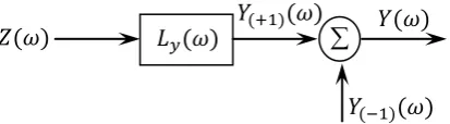
As illustrated in the schematic in Figure 5, the spectrum of the response can be

decomposed into a component which is correlated with the spectrum of the

nonlinearity through a frequency response function and a spectrum

which is uncorrelated with the nonlinearity, i.e.,

(19)

This is straightforward in the context of a single DOF and a single nonlinearity. In the

context of the general MDOF system with multiple nonlinearities considered in the first part

(20)

and in this case the decorrelation is an iterative process, sequentially removing the effects of

the nonlinearities from the vector response,

(21)

with the iteration beginning with,

(22)

The spectrum is thus conditioned by the removal of the influence of the first j

nonlinearities. Returning to the SDOF discussion, the ‘FRF’ function can be computed

using standard spectral estimation e.g.

(23)

If the spectrum of the input is similarly decorrelated with the nonlinearities,

(24)

(25)

the conditioned spectra can be used to form the FRF of the underlying linear system as if the

nonlinearities were not present.

In direct contrast to the CRP approach, the ORP method proposed here carries out the

decorrelation procedure directly in the time domain. If one applies the inverse Fourier

(26)

Suppose one is working with sampled data; assuming that the integral in equation (26) is

estimated from a discrete sum over samples where and is

the sampling interval, one obtains,

(27)

with the obvious definitions for the various symbols.

Equation (27) suggests that can be computed by sequentially removing the

correlating terms for from the measured response

Suppose the whole record of measured data for contains N sample points, where

One defines the vector as with a corresponding definition for

and for

With this notation, equation (26) implies,

(28)

with the introduced just to simplify the notation again. One can now regard the estimation

of as the problem of projecting onto the subspace of Euclidean space which is the

orthogonal complement of the space spanned by the , (denoted here by ). In order to do

this, it is necessary to establish an orthogonal basis on , (in fact, it might as well be

orthonormal), denoted where Such a basis can be computed by

(29)

(and there is another, largely irrelevant change of notation as the result of the change in

basis). One now defines a recursion based on,

(30)

where,

(31)

It is simple to show that if one starts the recursion with then it terminates

with the desired A similar recursion based on,

(32)

can be used to condition the input force signal in the time domain. Note that the conditioning

operations in the time domain depend on ‘future’ values of the signals and so this procedure

cannot be used online.

The conditioned (underlying linear) FRF can now be computed using standard

(unconditioned) spectral estimation methods on the conditioned input and output time-series.

The analysis for MDOF systems proceeds in exactly the same manner; however, it is

important to note that all suspected nonlinearities must be included in the equivalent of

equation (20) in order that the sequence of removals of orthogonalised nonlinear terms will

work. Once the conditioned FRF (or FRF matrix for MDOF) has been obtained, the

coefficients of the nonlinear terms can be estimated as in the standard CRP method discussed

6.

Application to Numerical Case Studies

To benchmark the performance of the new time domain (ORP) approach to the

identification of nonlinear systems, the first example considered here will be the standard

SDOF Duffing Oscillator (Example A in Figure 1 and Table 1) specified by equation (18).

The simulation time data were generated as before using a 4th-order Runge-Kutta scheme. The

excitation was a Gaussian white noise sequence with zero mean and RMS 10 N. The

time-step was 0.0005 seconds; 245760 points were generated in total. In order to compute spectra

the data were divided into 30 non-overlapping blocks for averaging and a Hanning window

was used.

The results from three different identification methods for the FRF are presented in Figure

6. The first approach used is a standard unconditioned FRF estimator, the second is the

frequency domain based CRP method (with the minor modifications suggested in Sections

3-4) and the third is the ORP method proposed here. The spectral estimation parameters were

those discussed above and the number of lags for the ORP approach was taken as

Excellent agreement with the true underlying linear FRF is obtained from both the CRP

and ORP methods; the lines are indistinguishable from each other in Figure 6. As one would

expect, the unconditioned estimate shows severe bias and fluctuations. Once the conditioned

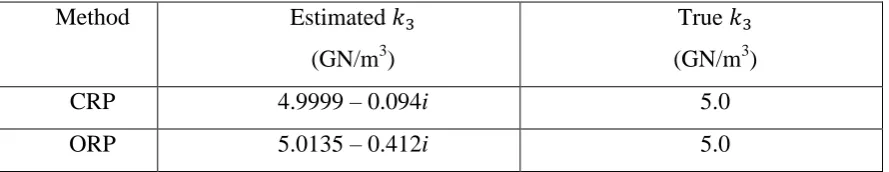
FRF is known, the nonlinear coefficient spectrum can be computed from,

(33)

The real and imaginary parts of the estimates are shown in Figure 7 for both the

CRP and ORP methods. As in the standard CRP approach, a single parameter estimate is

obtained by averaging the spectra (in this case, up to 25 Hz), the estimates for the CRP and

Method Estimated

(GN/m3)

True

(GN/m3)

CRP 4.9999 – 0.094i 5.0

ORP 5.0135 – 0.412i 5.0

Table 6. Comparison of the estimated coefficients for the Duffing system.

Figure 7 shows that the estimated coefficient spectra for the ORP approach descend into

high-frequency fluctuations well before and more severely than those from the CRP method;

however, with an appropriate upper cut-off for the spectral average, this is not an issue. If one

were to zoom the spectra of Figure 7 to cover the natural frequency, one would usually see

artefacts in the CRP results like those in Figures 4 and 9; however, because in this SDOF

case, the CRP appears to have produced a conditioned FRF free of artefacts, it produces a

slightly better estimate of than the ORP approach. However, the time domain ORP

approach has clearly proved successful for the SDOF Duffing oscillator; the next examples

are based on more taxing MDOF systems.

The first MDOF example considered is the 3DOF system B (Figure 1); this has a single

cubically nonlinear spring connecting the lowest mass to ground. The estimates of the

conditioned FRF for from the CRP and ORP methods together with the

unconditioned estimate are shown in Figure 8.

As in the SDOF case discussed above, the estimates of the conditioned FRFs from both the

CRP and ORP methods are excellent. Given the unconditioned (underlying linear) FRF

matrix (augmented by reciprocity as discussed in [12]), the standard CRP estimator for the

coefficient of the nonlinear term is found to be,

(34)

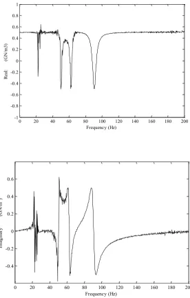
The corresponding coefficient spectra for the two methods are given in Figure 9. As in the

SDOF case, the spectra for the ORP approach descend into fluctuations before those from the

CRP method. However, if the spectral means are estimated over lower frequencies, the ORP

method gives a superior coefficient estimate of 1.00 + 0.01i GN/m3, compared to 0.81 – 0.07i

that the ORP spectra are free of the artefacts around the natural frequency as discussed earlier;

the errors in the CRP estimates arise as a result of these.

The final example considered here is the MDOF system, example D (Figure 1). This

system has nonlinear springs throughout. In order to estimate the nonlinear coefficients in this

case, one would have to use the recursive formula from [12] or consider the modified strategy

discussed earlier. As an alternative here, a simple least-squares approach is considered. As in

all cases, a good estimate of the conditioned (underlying linear) FRF is required. For

simplicity here, the idea will be illustrated by referring back to the Duffing oscillator case

(Example A). In the frequency domain, equation (18) becomes,

(35)

where and Assuming that spectral lines are available,

one has,

(36)

where and

contains the corresponding real and imaginary parts of the spectral lines from

Equation (36) can be solved using standard least-squares methods; of course, this

is not actually necessary in the situation here where there is only one parameter to estimate;

however, it becomes necessary in the multi-parameter MDOF case. An important aspect of

using this approach for parameter estimation is that the coefficient estimates are extracted

directly as real scalars and the spectral averaging is bypassed. A potential disadvantage of the

least-squares idea is that the CRP algorithm offers the potential (so far unexploited,

admittedly) of detecting frequency variation in coefficients; this is anticipated to prove

interesting in situations like viscoelastic material dynamics and is being investigated

currently. This means that one should only apply this least-squares approach if there is strong

a priori evidence that the coefficients are in fact constant. A further advantage of extracting the complete parameter spectra is that the resulting imaginary part provides a useful indicator

correct3

. For the current example, the underlying linear system was extracted using both the

CRP and ORP methods; the underlying linear systems for Examples B and D are the same, so

there is little point in a visual comparison of the unconditioned FRFs at this stage as the

extracted FRFs essentially coincided with those in Figure 7. As a numerical summary, Table 7

presents the identified resonance frequencies from the conditioned FRF estimates as

compared to the true values for the underlying linear system; the results are excellent. More

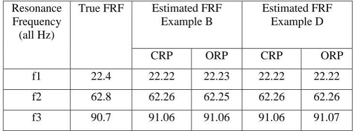
interesting perhaps, are the coefficients of the nonlinear terms, which were estimated as: 1.02,

0.97 and 1.02 GN/m3 for the three nonlinear springs in order from the base upwards. In

comparison with the true values of 1.0 GN/m3 in each case, the results are very good.

Resonance Frequency (all Hz)

True FRF Estimated FRF

Example B

Estimated FRF Example D

CRP ORP CRP ORP

f1 22.4 22.22 22.23 22.22 22.22

f2 62.8 62.26 62.25 62.26 62.26

f3 90.7 91.06 91.06 91.06 91.07

Table 7. The estimated resonance frequencies for the two examples of MDOF

nonlinear systems compared to true values.

7.

Conclusions

The CRP method offers a number of advantages as a means of nonlinear system

identification. It is certainly nontrivial with respect to its calculation but it also yields

information in a fairly intuitive form. The fact that the parameter estimates from the method

are returned in the form of a spectrum means that it offers potential for identifying

frequency-dependent systems, although this is not exploited here. Another benefit is that it allows one to

obtain the true FRF matrix (or part of it) of the underlying linear system by using conditioned

spectral analysis and this means that the nonlinear components of the response can be isolated

in a sense. One objection to the CRP method so far has been that artefacts from the

3

conditioned spectral analysis which yield the underlying linear FRF can corrupt or bias the

estimates of the nonlinear term parameters. The first objective of the current paper has been to

suggest some simple strategies for improving the parameter estimates for the nonlinear terms.

The basic ideas are (a) to bound the frequencies over which the parameter spectra are

averaged to exclude high frequency fluctuations, (b) to improve the coefficient estimates by

using weighting averages and (c) to estimate the parameters in isolation from each other in

order to avoid accumulation of errors due to recursion. The overall novelty of this work is

possibly in question as previous studies may simply have implicitly adopted these strategies;

however, the current authors feel there is some benefit in presenting a summary. Numerical

simulations have been carried out in order to study the influence of these strategies on the

parameter estimates and some benefit has been demonstrated. The actual origin of the

artefacts in the coefficient spectra as a result of the conditioning process and estimation of the

linear FRF matrix has not been discussed in any detail and further work is in progress on this

matter.

As a more radical approach to improving the conditioned spectral estimates, the second

and major objective of the current paper was to propose a means of carrying out the

conditioning in the time domain in order that completely standard unconditioned spectral

analysis could then be applied. This approach has been named here the Orthogonalised

Reverse Path (ORP) method. An advantage of the algorithm is that it can be coded in an

extremely transparent and compact form if an appropriate Gram-Schmidt module is available.

In this case a Matlab function orth was used. A minor disadvantage of using the packaged routine is that the memory demands in that particular case are high and this places restrictions

on the highest time-scale for decorrelation (encoded in the variable M here); this is currently under investigation. Some variants of the algorithm as described in [16] appear to alleviate the

problem. More generally, it would be useful to make a comparison between the computational

costs of the CRP and ORP algorithms; however, this is difficult because the algorithms are so

different in operation and depend on completely different hyperparameters. The CRP

algorithm depends on the size of the FFT window, number of averages etc.; the ORP

algorithm depends on the number of lags chosen. It would be difficult to decide what values

of hyperparameters for each algorithm gave comparable performance in order to then

compare computational cost. It is of course a very meaningful question and requires further

Apart from the conceptual clarity of the approach, the ORP method appears to produce

estimates of the nonlinear coefficient spectra which are free of the artefacts observed in the

CRP estimates in the vicinity of the resonance frequencies. This freedom from artefacts is a

clear advantage of the method; the reason for it is slightly unclear, and a detailed analysis of

the errors in the spectra is under investigation. Although the ORP estimates appear to be free

of the said artefacts; they degenerate into fluctuations at a lower frequency than the CRP

estimates, and this also is under investigation. Finally, as for all nonlinear system

identification methods, the final say on utility should be from experiment, and with this in

mind, experiments are currently underway.

Acknowledgements

The authors would like to thank the two anonymous reviewers for their constructive and

friendly comments; they believe that the paper has improved as a result of addressing the

References

[1]. Duffing, G., Errzwuhgen Schwingungen bei veranderderlicher Eigenfrequenz [Forced

Oscillations in the Presence of Variable Eigenfrequencies]. 1918: Vieweg,Braunschweig.

[2]. Kerschen, G., et al., Past, present and future of nonlinear system identification in structural

dynamics. Mechanical Systems and Signal Processing, 2006. 20(3): p. 505-592.

[3]. Allemang , R.J. and D.L. Brown, A unified matrix polynomial approach to modal

identification. Journal Sound and Vibration, 1998. 211: p. 301-322.

[4]. Busby, H.R., C. Nopporn, and R. Singh, Experimental modal analysis of nonlinear system: a

feasibility study. Journal of Sound and Vibration, 1986. 180: p. 415-427.

[5]. Ewins, D.J., Modal testing : theory, practice, and application 2000: Baldock : Research Studies Press.

[6]. Worden, K. and G.R. Tomlinson, Nonlinearity in Structural Dynamics : Detection,

Identification, and Modelling. 2000, Bristol: Institute of Physics.

[7]. Schetzen, M., The Volterra and Wiener Theories of Nonlinear Systems. 1980, New York: : John Wiley and Sons.

[8]. Rice, H.J. and J.A. Fitzpatrick, A generalised technique for spectral analysis of non-linear

systems. Mechanical Systems and Signal Processing, 1988. 2(2): p. 195-207.

[9]. Storer, D.M. and G.R. Tomlinson, Recent developments in the measurement and

interpretation of higher order transfer functions from non-linear structures. Mechanical

Systems and Signal Processing, 1993. 7(2): p. 173-189.

[10]. Adams, D.E. and R.J. Allemang, A Frequency Domain Method for Estimating The Parameters

of A Non-linear Structural Dynamic Model Through Feedback. Mechanical Systems and

Signal Processing, 2000. 14(4): p. 637-656.

[11]. Bendat, J.S., Nonlinear System Analysis and Identification from Random Data. 1990, Los Angeles, California: A Wiley-Interscience Publication, John Wiley & Sons.

[12]. Richards, C.M. and R. Singh, Identification of Multi-degree-of-freedom Non-linear Systems

under Random Excitation by the "Reverse path" Spectral Method. Journal of Sound and

Vibration, 1998. 213(4): p. 673-708.

[13]. Kerschen, G. and J.C. Golinval, Generation of Accurate Finite Element Models of Nonlinear

Systems-Application to an Aeroplane-Like Structure. Nonlinear Dynamics, 2005. 39: p.

129-142.

[14]. Marchesiello, Application of the Conditioned Reverse Path Method. Mechanical Systems and Signal Processing, 2003. 17(1): p. 183-188.

[15]. Kerschen, G., V. Lenaerts, and J.C. Golinval, Identificatin of a Continuous Structure with a

Geometrical Nonlinearity, Part 1: Conditioned Reverse Path Method. Journal of Sound and

Vibration, 2003. 262: p. 889-906.

[16]. Hoffmann, W., Iterative algorithms for Gram-Schmidt orthogonalization. Computing, 1989.

Figure Captions

Figure 1. Examples A, B, C and D: nonlinear systems.

Figure 2. Magnitude and phase of for Example (a) C and (b) Example D.

true estimate, unconditioned estimates.

Figure 3. Standard CRP estimates of for (a) Example C and (b) Example D.

conditioned estimate; unconditioned estimate.

Figure 4. Spectra for real and imaginary parts of nonlinear stiffness coefficient from

Example C.

Figure 5. Block diagram of reversed system model with uncorrelated input vector.

Figure 6. Unconditioned and conditioned (underlying linear) FRF estimates for Example A.

true FRF, H1 estimate, ORP estimate, CRP estimate.

Figure 7. Estimated spectra for the real (a) and imaginary (b) parts for of the nonlinear stiffness coefficient for Example A.

CRP estimate, ORP estimate.

Figure 8. Unconditioned and conditioned (underlying linear) FRF estimate for Example B.

true FRF, unconditioned estimate, ORP estimate,

CRP estimate

Figure 9. Estimate of the real (a) and imaginary (b) coefficient spectra for the nonlinear spring in Example B.

Figure 1. Examples A, B, C and D: nonlinear systems.

Cubic nonlinearity

Example B

Quadratic and cubic nonlinearities

Example C

K1

Cubic nonlinearity

Cubic nonlinearity

Cubic nonlinearity

Example D

Cubic nonlinearity

(a)

(b)

Figure 2. Magnitude and phase of for (a) Example C and (b) Example D.

true estimate, unconditioned estimates.

0 20 40 60 80 100 120

10-8 10-6 10-4 10-2 |H 21| ( m /N ) Example 1

0 20 40 60 80 100 120

-4 -2 0 2 4 Frequency (Hz) < H 21 (r ad) True H1 estimate

0 20 40 60 80 100 120

10-8 10-6 10-4 10-2 |H 21| ( m /N ) Example 2

0 20 40 60 80 100 120

(a)

(b)

Figure 3. Standard CRP estimates of for (a) Example C and (b) Example D.

conditioned estimate; unconditioned estimate.

0 20 40 60 80 100 120 140 160 180 200

10-8 10-6 10-4 10-2 |H 21| ( m /N ) Example 1

0 20 40 60 80 100 120 140 160 180 200

-4 -2 0 2 4 Frequency (Hz) < H 21 (r ad) H21(Unconditioned) H21(Conditioned)

0 20 40 60 80 100 120 140 160 180 200

10-8 10-6 10-4 10-2 |H 21| ( m /N ) Example 2

0 20 40 60 80 100 120 140 160 180 200

Figure 4. Spectra for real and imaginary parts of nonlinear stiffness coefficient from

Example C.

0 20 40 60 80 100 120 140 160 180 200

-1 -0.8 -0.6 -0.4 -0.2 0 0.2 0.4 0.6 0.8 1 Frequency (Hz) R ea l[  2] ( G N /m 3) Example 1

0 20 40 60 80 100 120 140 160 180 200

Figure 5. Block diagram of reversed system model with uncorrelated input vector. 

Figure 6. Unconditioned and conditioned (underlying linear) FRF estimates for Example A.

true FRF, H1 estimate, ORP estimate, CRP estimate.

0 10 20 30 40 50 60 70 80 90 100

10-4

10-2

M

agni

tude

(

m

/N

)

The Duffing FRF with different identification estimators

0 10 20 30 40 50 60 70 80 90 100

-4 -2 0 2 4

Frequency (Hz)

P

ha

se

(

ra

d)

(a)

(b)

Figure 7. Estimated spectra for the real (a) and imaginary (b) parts for of the nonlinear stiffness coefficient for Example A.

CRP estimate, ORP estimate.

0 10 20 30 40 50 60 70 80 90 100 -3 -2 -1 0 1 2 3 4x 10

10 Frequency (Hz) R ea l[ k3] ( G N /m 3) CRP ORP

0 10 20 30 40 50 60 70 80 90 100 -3 -2 -1 0 1 2 3 4 5 6x 10

Figure 8. Unconditioned and conditioned (underlying linear) FRF estimate for

Example B.

true FRF, unconditioned estimate, ORP estimate, CRP

estimate

0 20 40 60 80 100 120

10-7 10-6 10-5 10-4 10-3

Frequency (Hz)

|H

11|

(

m

/N

)

3DOF-1 at M=350

(a)

(b)

Figure 9. Estimate of the real (a) and imaginary (b) coefficient spectra for the nonlinear spring in Example B.

CRP estimate, ORP estimate.

0 20 40 60 80 100 120 140 160 180 200

-30 -20 -10 0 10 20 30 40 50 60 Frequency (Hz) R ea l [  3] ( G N /m 3 ) ORP CRP

0 20 40 60 80 100 120 140 160 180 200