Detection of damage of a filter by visualization of filtration process

a

[email protected], b [email protected]

Detection of damage of a filter by visualization of filtration process

P. Bílek1, a, P. Šidlof 1, b

1

Technical University of Liberec, Halkova 917/6, 460 01 Liberec 1, Czech Republic

Abstract. This paper deals with testing of filters on the basis of visualization of filtration process. A filtration material can be damaged by flow of the filtered medium, high pressure drop and long-term adverse conditions. These negative effects can cause extensive damage of the filtration textile and filtration efficiency decreases. The filter can be also fractured during manufacturing, processing or by improper manipulation. A testing of a purposely damaged filtration textile is described in the article. Experiments were performed on the filtration setup which permits an optical entrance to the position where a sample of filter is placed. A laser sheet is directed into this place. Scattered light from seeding particles in front of and behind the filter is captured by a digital camera. Images from the camera are analyzed and the filtration efficiency versus time and also versus position can be obtained. Measuring chain including light scattering theory and measuring of light intensity by a digital camera are also discussed in the article.

1 Introduction

One of the most important filtration parameters is the filtration efficiency. In this article, the filtration process is visualized in time and versus position. This testing method allows detecting local places with lower filtration efficiency and finding fractures in a filtration media.

Measuring chain including light scattering theory and measuring of light intensity by a digital camera are discussed in the article. A calibration constant of the measuring chain is calculated on the basis of simulations and also experimental measuring.

Non-woven filtration materials are used in wide range of industries. This paper is scoped on liquid filtration. The most important liquid filtration applications are in food, pharmaceutics, portable water, hydraulic oils, fuels and solvents. Therefore, many different kinds of filtration media which differ by materials, construction and performance characteristics are made. The filtration materials are used in a wide range of operating conditions. In many cases, polymers are used in production of filtration media and they are sensitive to mechanical, thermal and chemical attack. When a filter is damaged, the filtration efficiency decreases. The filtration properties can change suddenly or gradually during the filtration process and it is needed to detect the defects [1].

2 Measuring of filtration parameters

The most important performance characteristics of a filtration media are the filtration efficiency and pressure drop. Measuring of the filtration efficiency can be divided into two categories: offline and online. The output of the offline measuring method is one value at the end of an experiment. The online measuring method allows measuring the filtration efficiency during an experiment in time.

The most suitable measuring methods are based on optics. These methods are not invasive and they are sufficiently accurate. Concentration of particles in a medium is measured in reality and then the filtration efficiency

- (1)

is software calculated. The filtration efficiency EF[%] is a ratio between concentrations upstream C1[n/liter] and downstream C2[n/liter]. The pressure drop in [Pa]

Δp = p1 – p2 (2)

is a difference between pressures in front of the filter p1 and behind it p2.

C

2.1 Measuring of concentration of particles

2.1.1 Spectro-photometry

Spectro-photometry is based on measuring of colour intensity of a medium. The medium can be for example seeded up by colour particles. The more particles are in the medium, the higher colour intensity is detected by the spectro-photometer.

If the medium is air, particles can be burned and the intensity of flame colour is measured. For example, the particles of NaCl in air colour the flame into yellow colour. This method is very simple, but the output is only integral concentration of particles in time [3].

2.1.2 Optical particle counter

OPCs work on more principles according to size of detectable particles. Large particles can be detected by passing through a laser beam and making shadows on a sensor. This is an older light blocking measuring method. Modern methods are based on capturing the scattering light and the size range of detectable particles is much wider. OPCs are more complicated, but used very often. Outputs of this measuring method are concentration and size of particles (Particle Size Distribution) in the place where the optical probe of OPC is [4].

2.1.3 Phase Doppler anemometry

PDA measuring method is very similar to laser Doppler anemometry where only one detector is used. We measure by a measuring optical probe which arises by crossing two laser beams. In this place, the particles are detected. Scattered light by the particles is captured by at least two photo-detectors. The outputs are particle velocity, concentration, size and shape in the place where the probe is. More information is in [5].

2.1.4 Dynamic image analysis

The principle of this measuring method is the projection of particle shadows in transmitted light. The shadows of the particles are captured by two digital cameras. The first one captures whole scene and primarily large particles and the second one (zoom camera) detects small particles. The outputs are concentration, size and shape of particles. On the other hand, the area which is seen by the cameras is very small and the price for the machine is very high [6].

2.2 Particle image velocimetry

PIV is a measuring and a visualization method for investigation of a planar or volumetric velocity fields in gases and liquids. The very simplified principle is to illuminate seeding particles dispersed in a flow field with a laser sheet. A scene is captured by two laser sheet pulses separated by a time interval Δt[sec]. Images are captured by a CCD camera and divided into investigation

areas. The investigation areas of the first image are correlated with small areas of the second image.

A field of velocities

is calculated from the shifts of particles s[m] in the small areas and the time interval Δt[s].

In this article, only hardware arrangement is discussed, because the usage of this method for concentration measurement is interesting for us. Extensive image analysis is well described in the literature.

The laser sheet is made by laser beam and glass optics. Short pulse lasers (Nd:YAG) are the most effective due to their high light intensity and short light pulse, which does not heat the medium. In some cases of very low velocities, a continuous laser could be used.

The axis of the lens of a camera makes right angle with the laser sheet. Scattered light by the seeding particles falls on a CCD chip of the camera. The seeding particles are displayed as white points on a black background. The tracer particles have to be small enough to precisely follow the flow and at the same time large enough to scatter a lot of light [5].

2.3 Light scattering by small particles

Light scattering by small particles is very important issue which influences our measurements directly and it will be discussed in the article in the more detail.

Simplifying presumptions have to be determined to describe the light scattering. The first one is the scattered light has the same frequency as the incident light. Only elastic light scattering is discussed. The second presumption is sufficient distance of the particles from each other. Only independent scattering is considered. Then the scattering by one particle is possible to study. It means that N particles in a cloud scatter N times more light than one particle [7].

2.1.4 Light scattering by one particle

Particles are considered spherical, uniform and from isotropic material. Undefined formed particles are hardly describable by light scattering theories. Incident light is considered monochromatic and coherent (laser light).

Amount of scattered light in [W/m2]

is the wave number in [m-1]. The scattering angle θ[°] is between a source of light and an observer (Fig. 1.) and λ[m] is wavelength of the light source [7].

Figure 1 describes the situation of light scattering. Luminance in [cd/m2]

depends on reflectance of a surface ρ[-].

Figure 1. Light scattering by one particle [7].

More theories describe the scattering phenomena. The primary approaches are ordered according to size parameter

and relative refractive index

Diameter of the particle is Ø[m], refractive index of a material of the particle is npar[-] and refractive index of a medium is nmed[-].

Mie theory is the most complex and has no limitations of parameters x and m, but unfortunately it does not exist in a simple analytical representation. On the other hand, some software can calculate scattering diagram F(θ) according to input parameters. The biggest problem seems to be in the particles, in their material, shape, isotropy and surface. Real particles are not ideal and computation of the scattering diagram of a real particle is not very accurate.

2.1.5 Light scattering by N particles

We consider a medium with uniformly dispersed particles. The scattering diagram

of the illuminated volume Villu[m 3

] in the medium is equal to a sum of all scattering diagrams by N particles. Total luminance

of the illuminated particles is then proportional to concentration of particles in the medium C[n/m3] and scattering diagram of one particle F(θ).

represents the illuminated area in a real scene, which corresponds to the illuminated area on sensor As_illu[m2] and zoom factor of the lens Z[-].

Concentration of particles in [n/m3]

can be calculated from: total mass m[kg], density ρ[kg/m3] and diameter d[m] of the particles and total volume Vtotal[m3]. We consider the particles are small spheres.

2.4 Measuring of light intensity by CCD camera

Mechanisms of digital image generation will be explained here. Energy transmitted by electromagnetic waves is described by radiometric or photometric quantities. The radiometric quantities represent energy in whole spectrum of wavelengths. The photometric quantities express only light effect on human sight.

Light measurements are commonly performed by special devices. Illuminance E[lx, lm/m2] is measured by a lux meter (a photometer). It is density of a luminous flux Φ[lm] incident on a plane surface. Luminance or brightness of a light source L[cd/m2] is captured by a luminance meter. It is a luminous intensity I[cd] falling on unit area. This machine is more complicated and expensive. In reality, all the devices measure radiometric quantities (radiance Ee[W/m

2

] and irradiance Le[W/sr·m2]). Photometric quantities are calculated according to a spectral response of a human eye. A digital camera with CCD chip can serve as an illuminance or a luminance meter as well [8].

2.4.2 Lens

Very important component of a digital camera is lens which directly influences image quality. Lens has several parameters, the most important are focal length f[m] and aperture fap[-] (f-number of lens). Focal length in combination with the sensor size defines the field of view (angle of view)

Lens is not an ideal device and has several errors. Careful choice of the lens can partly decrease the errors. Wide angle lens distorts portraits and consequently the light intensity is not evenly distributed on a sensor. Distorted portraits are problematic with short focal length lenses. Some lenses can produce images with slightly darkened corners, especially when the aperture is wide open. This is vignetting and can be eliminated by closing down the aperture a little [9].

Irradiance of the sensor of a camera

is proportional to luminance of a light source L[cd/m2], transmission of all glass parts τ[-]. fap is f-number of lens.

2.4.1 CCD camera

A digital camera with CCD chip can serve as an illuminance or a luminance meter as well. This is very suitable in special cases where a light source is smaller than a sensor (for example testing of LED diodes). Another advantage is measurement of light intensity versus position, which is directly our case. In this application, it is necessary to utilize a digital camera with manual control allowed. That means a possibility of manual settings of shutter speed te[sec], aperture fk[-], focal length f[m], gain (amplification) G[-] and brightness YB[-]. The cameras which are running in automated mode cannot be used.

During exposure time (shutter speed) photons

fall through lens on a pixel Ap[m2] of the photosensitive sensor. Planck constant is h = 6.626·10-34 W·s2 and speed of light in vacuum is c = 2.998·108 m/s. Each photon (np[n] is number of photons) creates a free electron with a certain probability – quantum efficiency QE[%]. The pixel collects free electrons and forms a charge. Pixel has its own capacity and the charge is transformed into voltage

Ks[V/e

-] represents sensitivity of the sensor. Consequently, the voltage is amplified and digitalized and digital grey value of one pixel arises

Kadc[V/step] is resolution of A/D-converter and YB[-] is optional brightness of a picture in digital grey value. Detailed signal flow from light to digital numbers is described in the literature [9].

In other words, monochromatic digital camera converts irradiance of the captured scene L[cd/m2] into the digital grey value

of the pixel in an image. Kc[1/cd·sec] is a calibration constant of the camera and lens. The calibration constant is mostly experimentally measured with help of an integration sphere and a luminance meter. The accuracy of the calibration depends on the accuracy of the luminance meter used and properties of the integrating sphere. Calibration constant could be also calculated according to formulas (16) – (18).

2.4.3 Image file format

Most of the images from digital cameras are usually transformed into a compressed image format. Compressed images for example to the most famous JPEG format do not have linear function of pixel value versus the luminance due to the loss of information. On the other hand, the advantage of that is very significantly smaller size of the image and almost no difference compared to RAW image format for a human observer. RAW image format is lossless and stores the pixel values exactly as they were created by a sensor. Relationship between exposure value and pixel code is linear and this file format is suitable and preferred for light intensity measurement [9].

3

Filtration apparatus

Water filtration setup allows measuring pressure drop, flow rate and filtration efficiency. Optical measurement of the filtration efficiency is inspired by hardware arrangement of PIV method. Scheme is shown in figure 2 and a picture of the filtration setup in our laboratory is shown in figure 3. The filtration process is visualized by a laser sheet and captured by a camera with resolution 1920 x 1080 pixels. A traverse mechanism enables to measure the filtration process in the whole area of a sample of filtration media by movement with the laser sheet and the camera forward and back.

The filtration setup is composed of 3 circuits. Circuit 1 is very short and it serves for rough control of a flow and also for water mixing with artificial particles in a reserve tank.

Figure 2. Scheme of the filtration apparatus(1: Reserve tank for water, 2: Controlled pump, Ondina 50 T, P = 0.37 kW, 3: Manual ball valve, 4: Automatic air-escape valve, 5: Pressure sensor GMSD 3.5 BRE, Greisinger, 6: Pressure sensor GMSD 350 MRE, Greisinger, 7: Sample of a filtration material, 8 cm in diameter, 8: Glass tank for water, 9: Inductive flow meter M1500, Qmax = 10 liters per minute, Malema sensors,

10: Honeycomb screens, 11: Laser sheet, 12: Head with the laser unit, P = 50 mW, λ = 532 nm mounted on one axis traverse mechanism, 13: Manual ball valve, 14: Filter for cleaning of the apparatus, 15: Laser trap).

Figure 3. Picture of the filtration setup in laboratory.

Circuit 3 is activated only in case of cleaning of the filtration setup before a new measurement. The rest of the particles from the last measurements and other particles from tap water are removed from the setup.

3.1. Parameters of the filtration setup

The filtration setup allows setting the pressure drop in range 0 – 50 kPa and flow 0 – 25 liter per minute. It is also possible to set constant flow by use of PI regulator in a control unit of the pump and a flow meter. The round filtration chamber has 8 cm in diameter. The laser sheet is made by optics and a laser unit with a power of 50 mW is emitting continuous green laser light, λ = 532 nm. The

laser sheet is directed to the place where the filtration sample is mounted. Laser light is scattered by small artificial seeding particles in water. The scattered light is captured by the digital camera Pike F-210B/C with CCD sensor. Lens Nikon 50 mm with aperture F1,8 is placed on the camera. Signals from pressure sensors, flow meter and traverse mechanism are collected by NI data acquisition modules plugged in NI CompactDAQ – 9172 measuring central unit. The traverse mechanism and a triggering of the camera are controlled by MACA software written in NI LabView. Pictures are captured by AVT Smart View software.

4 Experiments

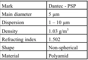
Experiments were performed by seeding particles which are described in table 1 in more detail. The seeding particles were used in mass concentration Cm = 1 mg/liter. Concentration is then C = 1.854 millions particles per liter according to formula (12) when we assume their spherical shape.

Table 1. Properties of seeding particles.

Mark Dantec - PSP

Main diameter 5 μm

Dispersion 1 – 10 μm

Density 1.03 g/m3

Refracting index 1.502

Shape Non-spherical

Material Polyamid

4.1 Calculation of a calibration constant

camera. The light is falling on a sensor and is transformed to a matrix of digital grey values = a raw image.

Figure 4. Block diagram of the measuring chain.

According to Mie theory, we simulated light scattering by one seeding particle in water. The polar graph was generated by MiePlot v 4. 3. 04, figure 5 [10]. The highest light intensity is in scattering angle θ = 0˚. Dimensionless function in scattering angle θ = 90˚ (where the camera is mounted) is F(90˚) = 68 [-].

Figure 5. Polar graph of light scattering by small particle [10].

According to formulas (9) – (18), digital grey value of the certain pixel in a camera

is directly proportional to concentration of particles C[n/m3]. Yoff[-] is offset and represents digital grey value of the illuminated place without any particles and had to

be experimentally measured. KT[m3/n] is the calibration constant and contains all parameters of the whole measuring chain.

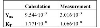
Ypx was calculated according to formulas (9) – (18) in Matlab software with sufficient accuracy. Input parameters of the laser light and the particles are shown in table 2 and extended parameters of the sensor and whole camera are explained in table 3. Finally, the calibration constant KT was calculated according to formula (20), table 4.

Table 2. Parameters of the laser light and the particles.

Intensity of the laser light E0 = 200 W/m2

Wavelength of the laser λ = 532 nm

Scattering function of the particle F(θ) = 68 Diameter of the particles d = 5 μm

Density of the particles ρ = 1.03 g/m3

Refracting index of the particles npar = 1.502

Refracting index of medium nmed = 1.333

Concentration of particles C = 1.854·10+6 n/liter

Table 3. Parameters of the sensor, lens and the camera.

Pixel size of the camera Ap = 7.4 x 7.4 μm

Resolution of the sensor 1920 x 1080 px

Zoom of the lens Z = 0.1

F-number of the lens fk = 1.8

Transmission + reflection of glass τ = 0.7

Planck constant h = 6.626·10-34 W·s2

Speed of light in vacuum c = 2.998·108 m/s Quantum efficiency (λ = 532 nm) QE = 36 %

Sensitivity of the sensor Ks = 14·10-6 V/e

-Sensitivity of A/D-converter Kadc = 8.54·10-6 V/step

Resolution of A/D-converter 16bit

Amplification G = 600

Brightness of a picture YB = 0

Table 4. Results of calculations.

Offset (DGV without particles) Yoff = 685

Digital grey value of one pixel Ypy= 9.544·10+3

Calibration constant KT= 1.771·10+8 m3/n

4.2 Measuring of the calibration constant

constant KT was calculated according to formula (20). Results are shown in table 5. Offset was experimentally measured and is the same as in previous case.

Table 5. Results of measurements

Offset (DGV without particles) Yoff = 685

Digital grey value of one pixel Ypx= 3.016·10+3

Calibration constant KT= 1.066·10+8 m3/n

4.3 Hole detection in a filtration material

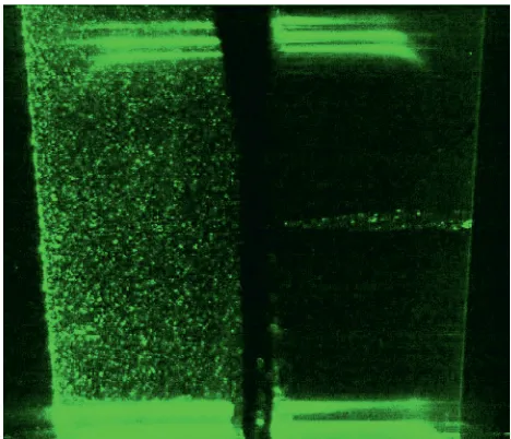
A sample of filter was tested in this article. The sample was made from 6 layers of microfibrous filtration textile, table 6. This sample was purposely damaged by a pin in the middle. The purpose was to find out if it is possible to detect the hole in the sample on the basis of visualization of filtration process.

Experiments were performed by the 5 μm artificial polyamid particles, table 2. Concentration was 1 mg per liter. 50 mg of seeding particles were dispersed in ethyl-alcohol by an ultrasound dispersant during 20 minutes to prevent agglomerates. The particles were added into 50 litres of cleaned tap water.

Table 6. Properties of the filtration material.

Laboratory name MB_A

Surface weight 120 g/m2

Technology meltblown

Material polypropylen

Diameter of fibers 2 – 5 μm

Structure 6 layers

4.4 Settings of the filtration setup

Flow rate of filtration media was set on 2.5 liters per minute and was kept constant during the whole experiment by PI controller. Settings of the camera were the same as in table 3. Such small seeding particles scatter very little of light. Therefore high amplification and slow shutter of the camera were set. The experiment took 15 minutes.

During the experiment, pressures in front of a filtration textile p1 and behind it p2 were measured. Pictures were captured by the digital camera in duration 6 pictures per minute.

4.5 Results

A picture of the filtration process is shown in figure 6. In the middle, the sample of a filtration textile is mounted. On the left side of the sample is upstream area and on the right side downstream area. We can see illuminated particles in upstream area of the filter. The particles are caught by the filter and only clear water

seeding particles go through the hole. We can see a stream of illuminated particles in downstream, figure 6. Flow behind the filter is laminar and the illuminated stream of particles is symmetric and straight.

Figure 6. Picture of the filtration process from the camera, 5 μm polyamide seeding particles.

Figure 7. Picture of the filtration process from the camera, glass 1.75 μm seeding particles.

The same damaged filtration textile was also tested by 1.75 μm, figure 7. Scattered light by such small seeding particles is very weak during the same mass concentration. Detection of any particles is almost impossible. We can see very weak illuminated stream of seeding particles in downstream of the filter caused by the hole.

In figure 8, pressure drop dp[kPa] versus time is shown and was calculated according to formula (2). We can see a significant break in the middle of the curve where the pressure drop increases more vertical. It is caused by increased flow via a filter on 10 liter/minute. Pressure drop increases in time because of fouling of the filter.

5 Summary

In many cases, polymers are used in production of filtration media and they are sensitive to thermal and chemical attack. One of the most important performance characteristic of a filtration media is filtration efficiency. It is measured mostly by optical particle counters or spectro-photometry.

The measuring method introduced allows detecting local places with lower filtration efficiency and finding fractures in a filtration media. The advantage of the method presented is that we can use it in special cases. For example, if the sandwich architecture of a filter is used, microscopy investigation methods cannot be used in this case. OPCs and spectro-photometry measure only integral values and can not detect the place with a hole.

The first goal of the article was to describe whole measuring chain. The digital grey value of one pixel Ypx in a picture from a digital camera is directly proportional to concentration of particles C. Calculated digital grey value Ypx = 9.544·10+3 is much higher than measured value Ypx = 3.016·10+3. Amount of scattered light was calculated for one seeding particle and multiplied by number of particles in illuminated volume. According to formula (20), a total calibration constant KT is possible to calculate. Consequently, the total calibration constant KT = 1.771·10+8 m3/n calculated on the basis of simulation and formulas (9) – (18) is different than experimentally measured KT = 1.066·10+8 m3/n, table 7.

Table 7. Results of the calculation and the measurement

Calculation Measurement Ypx 9.544·10+3 _3.016·10+3

KT 1.771·10+8 _1.066·10+8

This can be caused by more factors. Simulations of light scattering assume ideal seeding particles (spherical, homogenous, mono-disperse in size and non-absorbing light). In reality, the seeding particles used are not ideal and the scattering diagram can look very different. Also a part of light is absorbed by the seeding particles. The second significant factor should be homogeneity and power of laser sheet used. Ideal laser sheet has to be homogenous. In our physical setup, the intensity of light

is much stronger on the fringe than in the middle of the laser sheet.

The second goal of the article was a hole detection possibility in a filtration textile and visualization of filtration process. Two sizes of particles (5 μm and 1.75 μm) were tested during the same mass concentration Cm. According to the theory of light scattering, the light intensity decreases with smaller diameter. In Mie regime, the scattered light intensity decreases with square of particle diameter and in Rayleigh regime even with 6th power. A much stronger laser then 50 mW is needed for using of seeding particles smaller than 5 μm. Therefore the hole detection is guaranteed with usage of seeding particles larger than 5 μm with sufficient concentration.

Acknowledgments

This work was supported by the Ministry of Education of the Czech Republic within the SGS project no. 78001/115 on the Technical University of Liberec.

References

1. Lydall-filtration and separation, Nonwoven liquid filtration media – construction and performance

(2013), [online 20.6.2013], < http://www.lydallfiltration.com>.

2. A. Rushton, A. S. Ward, R. G. Holdich, Solid-liquid filtration and separation technology, VCH Verlagsgesellschaft mbH, ISBN: 3-527-28613-6 (1996).

3. J. Hrůza, Zlepšování filtračních vlastností

vlákenných materiálů, Technická universita v

Liberci, Liberec, p. 80 (2005).

4. T. Harrison, B. Latimer, ISO 21501/A standard merthodology to optical particle counter calibration and what it means to clean room owners, Hach Ultra Analytics (2008), [online 20.6.2013],

< http://www.hach.com>.

5. V. Kopecký, Laserové anemometrie, Liberec, p. 186, ISBN: 9788070839454 (2006).

6. Horiba company, Dynamic image analysis technology, [online 20.6.2013],

<http://www.horiba.com/scientific/products/particle -characterization/technology/dynamic-image-analysis/>.

7. H. G. van de HULST, Light Scattering by Small Particles. Willey, New York (1957).

8. P. D. Hiscocks, P. Eng, Measuring luminance with a digital camera, Syscomp electronic design limited, p. 25 (2011).

9. F. Dierks, Sensitivity and image quality of digital cameras, Basler Vision Technologies, p. 36 (2004). 10. P. Laven, MiePlot software, [online : 22.7.2013],