Generalized decomposition and cross entropy methods for many-objective optimization

many-objective optimization

.

White Rose Research Online URL for this paper:

http://eprints.whiterose.ac.uk/74767/

Monograph:

Giagkiozis, I., Purshouse, R.C. and Fleming, P.J. (2012) Generalized decomposition and

cross entropy methods for many-objective optimization. Research Report. ACSE Research

Report no. 1029 . Automatic Control and Systems Engineering, University of Sheffield

[email protected] https://eprints.whiterose.ac.uk/ Reuse

Unless indicated otherwise, fulltext items are protected by copyright with all rights reserved. The copyright exception in section 29 of the Copyright, Designs and Patents Act 1988 allows the making of a single copy solely for the purpose of non-commercial research or private study within the limits of fair dealing. The publisher or other rights-holder may allow further reproduction and re-use of this version - refer to the White Rose Research Online record for this item. Where records identify the publisher as the copyright holder, users can verify any specific terms of use on the publisher’s website.

Takedown

If you consider content in White Rose Research Online to be in breach of UK law, please notify us by

Generalized Decomposition and Cross Entropy

Methods for Many-Objective Optimization

Ioannis Giagkiozis, Robin C. Purshouse, and Peter J. Fleming,

Department of Automatic Control and Systems Engineering

The University of Sheffield

Research Report No. 1029

November 2012

Abstract—Decomposition-based algorithms for multi-objective optimization problems have increased in popularity in the past decade. Although their convergence to the Pareto optimal front (PF) is in several instances superior to that of Pareto-based algo-rithms, the problem of selecting a way to distribute or guide these solutions in a high-dimensional space has not been explored. In this work, we introduce a novel concept which we call generalized decomposition. Generalized decomposition provides a framework with which the decision maker (DM) can guide the underlying evolutionary algorithm toward specific regions of interest or the entire Pareto front with the desired distribution of Pareto optimal solutions. Additionally, it is shown that generalized decomposition simplifies many-objective problems by unifying the three performance objectives of multi-objective evolutionary algorithms – convergence to the PF, evenly distributed Pareto optimal solutions and coverage of the entire front – to only one, that of convergence. A framework, established on generalized decomposition, and an estimation of distribution algorithm (EDA) based on low-order statistics, namely the cross-entropy method (CE), is created to illustrate the benefits of the proposed concept for many objective problems. This choice of EDA also enables the test of the hypothesis that low-order statistics based EDAs can have comparable performance to more elaborate EDAs.

Index Terms—Generalized decomposition, cross entropy method, MACE, many-objective optimization, multiobjective op-timization, decomposition methods, scalarising functions.

I. INTRODUCTION

M

min

x F(x) = (f1(x), f2(x), . . . , fk(x))

subject to x_∈S, (1) where k is the number of objective functions and x is the vector of decision variables defined in the domain S _⊆Rn_.

It should be clarified what we mean by the notation min x is

minimization over x which is different to the min operator which returns the minimum element of a set. We follow this convention because it leads to a more compact description. There is an implicit assumption that the scalar objective functions are competing, since if this assumption is not true then (1) degenerates to a single objective problem, or if some The authors are with the Department of Automatic Control and Systems Engineering, University of Sheffield, Sheffield, UK, S1 3JD.

E-mail: [email protected]

of the k objectives are competing and some are harmonious then the effective number of objectives will be less than k [4]. MOPs for 2 or 3 objectives have been heavily studied, however there is the need for algorithm frameworks that can deal with higher dimensional problems, i.e. more than 3 objectives. These problems are so-called many-objective problems (MAPs), for brevity we refer to multi and many-objective problems simply as MAPs.

The problem that is apparent in MAPs is that there is no

natural way of ordering the obtained solutions; this ordering

is crucial for fitness assignment. However MOEAs base their

decision as to the direction of search on the assigned fitness of

various solutions in the population. This is a very well known problem in MAPs and has been addressed with varying degrees of success by a number of researchers over the past three decades [5]–[7]. In general there are two approaches employed to resolve this issue: Pareto-based and decomposition-based methods. In both methodologies there is the assumption that the relative importance of the objectives is unknown. In the case that this information is given by the decision maker (DM) then a decomposition method can be used to create a scalar objective function, see Section III.

Pareto-based methods use the Pareto-dominance relations [8], to induce partial ordering in the objective space. These relations, were initially introduced by Edgeworth [9] and later expanded by Pareto [10]. For example for two vectors

a,b _∈ Rn, a b if all the elements in a are smaller or equal (_≤) to the corresponding elements in b and at least one element inais strictly (<) smaller than its corresponding element inb. This partial ordering, induced by therelation, is denoted as a b, and, in the context of a minimization problem this expression is read as: the vectora dominatesb. For a more complete treatment of Pareto-dominance relations the reader is referred to [8]. However such relations are of limited utility when the number of dimensions is increased [11]. This is primarily because the number of non-dominated solutions increases as the dimensionality of the problem in-creases, and for dimensions greater than around ten, almost all the solutions are non-dominated [12]. Hence this type of partial ordering becomes of limited use in high dimensions since, if all the generated solutions are non-dominated, the EA has no objective measure on which to base its selection process.

func-tion to aggregate all the objectives into a single objective function. Such methods have been used predominantly in non-linear mathematical programming, where the main algorithm is based on some variant of gradient search [8], [13]. However multi-objective evolutionary algorithms (MOEAs) have also employed decomposition with varying degrees of success, for example [14]–[16]. Arguably, decomposition methods have not been explored to sufficient depth for MAPs. For example, a popular hypothesis, that is employed by several MOEAs, is that an even distribution of weighting vectors will result in well distributed Pareto optimal points [7]. However, with the help of a novel concept which we call generalized de-composition, we show that this assumption is fundamentally flawed and we provide an exact solution to this issue, subject to some prior information. It is interesting to note that recently several researchers have taken an interest in the selection of weighting vectors in decomposition-based methods. For instance [17] identify two issues with the way that set of weighting vectors are selected in MOEA/D [7]: (i) it is not possible to select an arbitrary number of weighting vectors, which can be problematic for many-objectives, and, (ii) the number of weighting vectors situated on the boundary tends to be large. The boundary in this context is understood to mean: weighting vectors with many components equal to zero. Weighting vectors on the boundary produce subproblems that completely disregard some of the objective functions which in general is undesirable [17]. The suggestion is to use uniform

design to select the set of weighting vectors instead of a set

of evenly distributed weighting vectors. However, as is shown in this work, an even or uniform distribution of weighting vectors does not produce evenly distributed Pareto optimal solutions, hence what is proposed in [17] does not address the more pressing issue, that of finding the distribution of weighting vectors that would lead to a Pareto set whose points have a desirable distribution on the PF. This distribution can be defined in numerous ways, and depends mostly on the preferences of the DM. This issue is further discussed in Section III-C.

An interesting adaptive method to select the set of weight-ing vectors is presented in [18], [19]. The main idea is to identify the Pareto front geometry and then distribute a set of points on that surface in such a way so as to maximize the hypervolume indicator [20]. Subsequently, the points found in the previous step, are used to identify a weighting vectors that, upon minimization of the resulting subproblems, would result in similar points on the Pareto front. The idea seems hopeful, however, there are three major difficulties with this approach. First, the authors assume that the Pareto front can be parameterized using the following,

fp1

1 +f

p2

2 = 1, (2)

where, pi ∈ R++ and the fact that (2) equals to one means

that the objective functions are normalized in the range,[0,1]. The problem is that (2) is nonconvex but the authors of [18], [19] ignored this issue and used the Newton method to solve for thepi parameters. Therefore, if there is noise in the Pareto

optimal points used in identifying the pi parameters or the

Pareto front geometry has, pi 6=pj, i 6=j, this method will

fail. This can be seen in [19] whereby a front described by: f2

1 +f2= 1is generated and the estimate using the Newton

method is: f1.445

1 +f21.445 = 1. Therefore, the first part of

the suggested method can mislead the entire procedure in [18], [19]. The second problem, is that the weighting vectors that correspond to points on the identified Pareto front are formulated in a similar fashion to (2), hence the issue of nonconvexity of the problem formulation emerges again and the resulting weighting vectors will not produce subproblems that converge to the reference points. Lastly, the hypervolume indicator [20], which is used to ascertain the quality of the

reference points on the PF, has exponential complexity in the

number of objectives [21], [22], which limits the method to approximately 4-objective problems, since the hypervolume must be calculated several times on every iteration of the algorithm [19].

Most tantalizingly, in a recent publication Gu et al. [23] discuss a solution for identifying a weighting vector set using a set of evenly distributed Pareto optimal solutions. However, the proposed method in the above mentioned work is limited for the weighted sum method and the Chebyshev scalarizing function [23]. For example if weakly Pareto optimal solutions are to be avoided, the modified Chebyshev scalarizing function [8, pp. 101] can be used. However there is no clear way in identifying the required set of weighting vectors using the proposed methodology in [23].

Evolutionary algorithms (EAs) have found numerous ap-plications in MAPs [12]. This is because most EAs are population-based, in the sense that at each iteration an entire population of solutions is evaluated. This feature is quintessen-tial to MAPs since, in a posteriori optimization, an entire family of solutions is required to describe the trade-off surface. This trade-off surface in objective space is also called the Pareto front (PF). Another important reason for EA applica-bility is that they impose almost no constraints on the problem structure; for example, continuity and differentiability are not required for EA operation. Due to these factors MAP research is vibrant in the EA community, something that can be attested by the number of EAs available for MAPs, e.g. [7], [12], [24]. Specifically EAs are comprised of a number of algorithm families, such as genetic algorithms (GAs) [25] and evolution strategies (ES) [26], as well as differential evolution (DE) [27] and others. Most of the aforementioned algorithm families are inspired by some naturally occurring process, such as DNA recombination and mutation [25]. However this presents certain difficulties. For example, it is very hard to analyse the behaviour of MOEAs analytically, thus their performance on a problem cannot be guaranteed prior to application. This is why EAs are usually evaluated experimentally using some test problem sets [28]–[30].

new population of better1 _{individuals. From the EA point of} view, EDAs can be traced back to recombination operators based on density estimators that use good performing individ-uals in the population as sample [31]. A positive aspect of EDAs is that it is straightforward to fuse prior information into the optimization procedure, thus reducing the time to convergence if such information is available. Also, the amount of heuristics, compared with other EAs, is reduced easing the task of mathematical analysis of these algorithms. This is an important aspect which has been overlooked, due to inherent difficulties, in most heuristics for optimization. Studies of this kind are usually applied to algorithms that are not used in practice [32], [33], therefore the practical value of such studies is limited. However EDAs are not a panacea since they heavily depend on the quality and complexity of the underlying probabilistic model [34]. For instance, a simple EDA based on low-order statistics, i.e. an EDA that does not account for variable dependencies, can be easily misled if, in fact, such dependencies exist in the underlying problem. To overcome such difficulties researchers proposed ever more elaborate models [34], which of course increase the complexity of the algorithm and in some instances the identification of the optimal model is of comparable complexity to that of the optimization problem necessitating the use of heuristics [35]. Acknowledging this problem has led some researchers to suggest hybridization of EDAs based on simple probabilistic models with some form of clustering [36]. This course is further supported by more recent studies [37].

For these reasons we have selected an optimization algo-rithm, the so-called Cross Entropy method (CE), as the main algorithm in our generalized decomposition-based framework. The CE-method was introduced by Rubinstein [38], initially as a rare event estimation technique and subsequently as an algo-rithm for combinatorial and continuous optimization problems. The most alluring feature of CE is that, for a certain family of instrumental densities, the updating rules can be calculated analytically, and thus are extremely efficient and fast. Also the theoretical background of CE is enabling theoretical studies of this method which can provide sound guidelines about the applicability of this algorithm to problems.

The main contributions of this work can be summarized as follows:

• A generalization of decomposition methods is presented,

that is applicable to a wide range of EAs and for all scalarizing functions that are convex with respect to the weighting vectors. Using the presented methodology, the spread of the resulting PF can be directly controlled. Additionally, it is shown how generalized decomposition can be used to refine the search of a MOEA in regions that are of particular interest to the DM, thus introducing preference articulation for decomposition methods.

• Using generalized decomposition, the CE-method is

ex-tended to MAPs and is shown to perform very well compared to two other EAs, namely MOEA/D, RM-MEDA, and random search.

1_{Or more precisely, individuals that are more likely to be better than their} predecessors.

The remainder of this paper is structured as follows. In Section II we elaborate on the ensuing problems in Pareto-based methods for many objective problems. In Section III generalized decomposition is described along with the benefits that this method can bring to currently existing MOEAs. Following this, in Section IV the CE-method is presented along with its form for continuous optimization problems. A many-objective optimization framework based on generalized decomposition and the CE-method is presented in Section V. The algorithms in our comparative studies in Section VII are described in Section VI. In Section VIII we illustrate how generalized decomposition can be used for preference articulation. Lastly in Section IX we summarize and conclude this work.

II. PARETO-BASEDMETHODSANDMANY-OBJECTIVE PROBLEMS

The concept of Pareto-dominance is of limited use as a fitness assignment scheme for many-objective problems. Of course, Pareto-optimal solutions in any number of dimensions will still be the minimal elements of the feasible set in objective space. In [39] a very interesting geometric argument is presented that should clarify this point. In what follows we elaborate on the above mentioned argument.

Consider the simplest multi-objective case, namely a 2 -objective problem. Every point in -objective space defines 4

regions, (i) a region that contains solutions that are clearly bet-ter, (ii) a region that contains solutions that are clearly worse and (iii, iv) two regions where the solutions are incomparable to the point in question. Now, for3-objective problems there are8such regions (23_{), however there is only1region which}

contains clearly better solutions and 1 region with clearly worse solutions. So, there are23

−2 = 6regions that contain solutions incomparable to the point in question. In general the following is true, fork-dimensional problems, there is always

1 region with clearly better solutions, 1 region with clearly worse solutions and 2k

−2 regions containing incomparable solutions. Now, assuming that there is no bias towards any of these regions in the problem (objective function), the probabil-ity that a solution is generated in any one of these regions by a stochastic process (algorithm) is approximately proportional to the volume of these regions divided by the volume of the entire feasible set in objective space2. However, for increasing number of dimensions, the likelihood that a solution will be generated within the region of solutions that are clearly better becomes almost insignificant the closer the point is to the Pareto front [39]. For example, for 11 dimensions there are

2 048 regions, hence for the above problem, the probability for a solution to be generated, that dominates the current point, is approximately p = 1/2 048 = 4.88−4 _{if the point}

in question is exactly in the middle of the feasible objective set. To contrast this, the probability that a non-comparable solution is generated is2 046/2 048_≈0.99.

However, we have simplified the problem greatly, that is we have assumed no bias and that the point is significantly away from the Pareto front so that the volume of all the regions

f1

f2

f3

w1

w2

w3

0

0.5

1 0

2 4

0

0.5

1 0

2 4

0

0.5

1

0 2 4

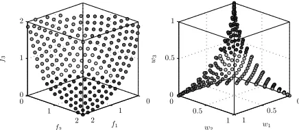
Fig. 1. Left: An affine Pareto front. Right: The corresponding optimal weighting vectors. Different shades of grey aid in identifying corresponding regions in the Pareto front and the associated weighting vectors.

f1

f2

f3

w1

w2

w3

0

0.5

1 0

1 2

0

0.5

1 0

1 2

0

0.5

1

0 1 2

Fig. 2. Left: A concave Pareto front. Right: The corresponding optimal weighting vectors.

is approximately the same. Naturally, this is highly unlikely to be the case, so let us consider a more realistic scenario. Let the problem in question be bounded, so assuming we know the boundaries, we can shift it so that its forward image (objective space) is the nonnegative orthant. The only case that the problem will be easier to solve, is when there is bias towards the Pareto front, but this is not usually encountered in practice. The contrary is a much more common situation, namely that there is “resistance” in finding better solutions. This combined with the fact that as a solution approaches toward the Pareto front the region that contains clearly better solutions is becoming very small, the probability that a worse solution is generated is increasing toward p → 1 (no-bias towards worse solutions) and the probability of generating a better solution is diminishing toward p → 0. Regarding the regions that contain incomparable solutions, their volume is exchanged with the region that contains clearly worse solutions. Therefore it becomes increasingly more difficult to find solutions in the desirable direction.

The difference with decomposition-based algorithms is that, for each subproblem a complete ordering of the objective space is defined, irrespective of its dimension. This in effect reduces3 _{the rate of decrease of the probability that a better} solution is generated [39]. To see this consider a scenario that the weighted sum method is used (see (3)). In this scenario the weighting vector represents the normal of a hyperplane that separates the feasible objective space in two regions. One region containing better solutions and one with worse solutions. Solutions above the hyperplane are considered to be worse while solutions below the hyperplane are taken to

3_{This statement is true only for the weighted sum scalarizing function. For} other scalarizing functions a more elaborate formulation is required, however there are indications that a similar statement may be established [39].

f1

f2

f3

w1

w2

w3

0

0.5

1 0

1 2

0

0.5

1 0

1 2

0

0.5

1

0 1 2

Fig. 3. Left: A convex Pareto front. Right: The corresponding optimal weighting vectors.

be better with respect to the particular subproblem [39]. An intuitive way that explains why this is the case is if we consider the effect of a scalarizing function to the objective space. A scalarizing function projects the entire objective space onto a line4_{, therefore some regions that contain incomparable} solutions in the Pareto sense, now become solutions that are either better or worse for the particular subproblem. Admittedly this is not an entirely desirable behaviour, however the algorithm is provided with an unambiguous direction of search. It should be noted that by using a decomposition-based method, the problem does not become any easier to solve. The major difference between decomposition-based and Pareto-based algorithms is that the former provide unambiguous information about the quality of the produced solutions at every iteration while the latter cannot always guarantee such information because the likelihood of generating incomparable solutions in high dimensions is high [12]. However it is easy to reduce the above argument into a zugzwang between Pareto-based methods and decomposition-based methods. This is accomplished by the simple observation that the clearly

better regions in the Chebyshev scalarizing function (see (5))

are identical to the regions generated by Pareto dominance based methods, while the incomparable and clearly worse regions in Pareto-based methods are mapped to clearly worse regions by the Chebyshev scalarizing function. Namely, if we require a decomposition method that can guarantee the generation of Pareto optimal solutions, then, we have to use the Chebyshev scalarizing function but in so doing we give up the favourable convergence rates5 achieved when using the weighted sum method, and vice versa. There are ways that different scalarizing functions can be used to adaptively resolve this issue while preserving the guarantees that the Chebyshev function provides however this requires further investigation.

III. GENERALIZEDDECOMPOSITION

A. Decomposition Methods

Decomposition methods, or so-called scalarizing functions, have been employed in several MOEAs, for example [14]– [16]. These methods transform (1) to a single-objective prob-lem by combining the objective functions to form a single scalar objective function. The potential of such methods for extending MOEAs to MOPs is obvious considering the basis

Number of Objectives

lo

g10

(

E

m

E

(

E

b

)

)

Generalized decomposition Evenly distributed weighting vectors Uniformly distributed weighting vectors

Expected energy of uniformly distributed Pareto solutions

2 3 4 5 6 7 8 9 10 11

-12 -10 -8 -6 -4 -2 0 2 4 6 8 10 12

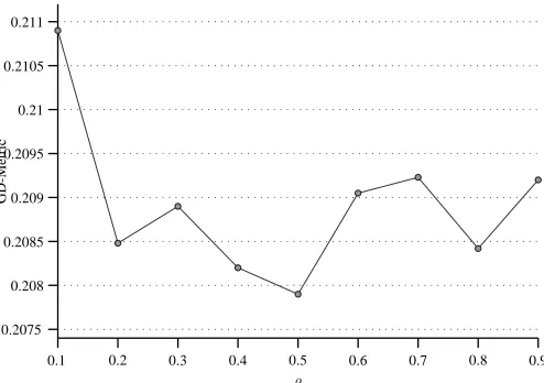
Fig. 4. Logarithm of the energy ratio of generalized decomposition, evenly distributed weighting vectors [7], and uniformly distributed weighting vectors [14].

of almost every, if not all, optimization algorithms is a method that can address only single objective problems. Therefore decomposition methods present a clear path in extending such algorithms to MOPs.

Arguably the simplest scalarizing function is the weighted sum method [40]:

min

x w

T_F(x) k

X

i=1

wi= 1, andwi ≥0,∀i∈ {1, . . . , k},

(3)

wherew= (w1, . . . , wk). However it has been shown that for

complicated Pareto fronts, an algorithm based on (3) is unable to discover all Pareto optimal solutions [8]. Although, with some modifications this simple decomposition can produce respectable results, for example see [7].

A more sophisticated decomposition is based on the weighted metrics method [40]:

min x

k

X

i=1

wi|fi(x)−zi⋆|p

!p−1

, (4)

here as in (3), it is assumed thatwi≥0and thatPki=1wi= 1,

and p ∈ [1,∞). Also z⋆ is the ideal vector, which is equal to the minimum values for all the objectives independently. When p → ∞ the well known Chebyshev decomposition is obtained:

min

x kw◦ |F(x)−z

⋆

| k∞. (5)

The _◦ operator denotes the Hadamard product which is element-wise multiplication of vectors or matrices of the same size. This decomposition is quite interesting due the fact that there are theoretical results stating that for any Pareto optimal solution ˜x there exists a convex weighting vectorw

for which the solution of (5) is x˜ [8]. Note that by, convex weighting vector, w, we mean a vector w_∈convC, where

C=_{ei:i= 1, . . . , k}andei is a vector whose components

are all equal to zero, except its ith _{component that is equal}

to one. Also convC is the convex hull of the set C which is defined in (37). For further details see Appendix B. This means that all Pareto optimal solutions can be found using the Chebyshev decomposition. This result is very encouraging, however it does not suggest a way to choose the weighting vectorsw in order for a representative and evenly spread PF to be obtained.

B. Optimal Choice of Weighting Vectors

The guarantee that all Pareto optimal solutions can be obtained by the Chebyshev decomposition, for some convex weighting vectorw, is well known and has been exploited on numerous occasions in past research. For example Jaszkiewicz [14] suggests that a uniformly sampled set of weighting vectorswshould produce uniformly distributed Pareto optimal solutions along the entire PF. Later Zhang et al. [7] argue that choosing at each iteration a new random weighting vector is too ambitious, since only an approximation of the PF is necessary. Instead the authors suggest that a set of evenly spaced weighting vectors should produce well distributed Pareto optimal solutions. Their main argument was that this should be the case since the various subproblems obtained using different weighting vectors are a continuous function of the weights [7]. This seems to be the case, however there is nothing to suggest that this continuous function is also linear in the parametersw, which is the only case for which their assumption would hold, up to a multiplicative constant. Namely, an evenly distributed set of weighting vectors would produce well distributed Pareto optimal solutions only in the case that the functiong∞(·)defined as:

min

x g∞(x,w

s_,z⋆_{) =}

kws_{◦ |}F(x)₋z⋆_{| k}∞

∀s={1, . . . , N}, subject to x_∈S,

(6)

is linear in the weights w, which is obviously not the case. The parameterN in (6) is the size of the population which is equal to the number of subproblems to be solved and ws _is

the weighting vector of thesth _subproblem.

kw˜_◦F(˜x)_k∞≤ kw◦F(˜x)k∞for all convex vectorsw. This

means, that for all possible subproblems defined by the set of weighting vectorsw_{∈ W}, the Pareto optimal solutionF(˜x)is

closest to the subproblem defined by the weighting vector w˜. Closest in this context means that the Pareto optimal solution,

F(˜x), minimizes the subproblem defined byw˜. Additionally, W is the set of allkdimensional convex vectors. The ability to obtain the weighting vectorw˜ for a particular point on the Pareto front can be exploited in several ways as explained later in this section. To obtain thew˜ vectors, the following program is to be solved for every Pareto optimal point of interest:

min

w kw ◦ F(x)k∞,

subject to

k

X

i=1

wi= 1,

andwi≥0,∀i∈ {1, . . . , k}.

(7)

Also to obtain the optimal weighting vectors for the weighted metrics scalarizing function for p other than infinity, all that is required is to change the norm in (7) to reflect that change. If the scalar objective functions (f1(x), . . . , fk(x)),

that comprise the objective vectorF(x), are non-negative for all x_{∈ S} then the problem formulated in (7) is a disciplined convex program [41], hence it is also a convex program. So a unique solution is guaranteed and can be obtained by solving (7) using some interior-point method [42]. On a side note the non-negativity constraint on the scalar objective functions can be relaxed in the case that all scalar functions are bounded from below and these lower bounds are known. In which case

F(x)is replaced by,

˜

F(x) = (f1−b1, . . . , fk−bk), (8)

wherebi are the respective lower bounds for the scalar

objec-tive functionsfi. For details on the formalism of disciplined

convex programming, the interested reader is referred to [41]– [43].

The general idea is that the generation of weighting vectors greatly influences the convergence and spread of the resulting Pareto front. However, this selection has been either arbitrary [14], or based on invalid assumptions [7]. Additionally, the method presented by MOEA/D (see Section VI-A) to gener-ate weighting vectors is limiting in the sense that for high dimensional problems the choice of the size of the population is restrictive. For example, for H = 10, where H can be interpreted as the number of divisions per dimension for the weighting vectors, and for 11 objectives the population size must be equal to 92 378. This H setting is less than half of that used by Zhang et al. [7] for 3-objective problems. This restriction can prove problematic in certain situations, for example if a different choice of population size is more natural or if there are computational and memory constraints.

C. The Effect of Weighting Vector Choice

Assuming that our definition of well distributed PF solutions is a Pareto optimal set uniformly distributed along the trade-off surface, the following experiment illustrates the benefits of using generalized decomposition. It should be noted that

the generalized decomposition framework is fully capable of accommodating any other definition of well distributed Pareto optimal solutions. A commonly used measure of evenly distributed points on the unit hypersphere is the Coulomb potential [44], or Riesz kernel [45], defined as:

E(Z;s) = X

1≤i≤j≤N

kzi−zjk−s,s >0

z_∈Rk, and,Z=_{zi:i∈ {1, . . . , N}},

(9)

and fors= 2, (9) is equivalent, up to a multiplicative constant, to the Coulomb potential energy. The set Z in the present work is the set of objective vectors z. Intuitively, when (9) is minimized then the mean nearest neighbour distance of the set of points z is maximized, subject to the constraints imposed by the geometry of the PF. For some examples on the distribution of solutions using (9) the reader is referred to [44]. We illustrate the fluctuation of energy for an increasing number of dimensions, when the weighting vectors are chosen either according to the suggestions in [14] or [7], see Fig. (4). It should be noted that these schemes for weight vector selection are predominantly used in several algorithms. The results in

Fig. (4) have been obtained in the following way:

• For2to11dimensions and for a concave PF, N number

of objective vectors are selected according to generalized decomposition and the methods described in [14] and [7]. The number of selected objective vectors used in every instance can be seen in Table I. This choice is motivated by the fact thatH is the number of subdivisions per dimension, so the point density of objective vectors for a constant H should represent the PF equally well, in all dimensions. The H parameter has been set to 7

because for11objectives the number of objective vectors, N, increases quite rapidly for a higher value of H. For instance, for H = 8 and H = 9 the number of objective vectors becomesN = 19 448andN = 43 758

respectively. This increases the computational resources required for the experiment significantly.

• For each problem instance, a set of weighting vectors was

generated according to the proposed methods in [14] and [7]. For generalized decomposition the weighting vectors are generated using a reference Pareto front with the desired distribution. For example, in2dimensions the first quadrant of a unit circle is uniformly sampled and then the optimal weighting vectors are estimated by solving (7). Also the expected energy E(Eb) is calculated using

N _×50 independent uniformly distributed samples on the PF. Details on the generation of a uniformly sampled concave PF can be found in Appendix A.

• Subsequently, using the inverse relationship to (7),

TABLE I

THE NUMBER OF OBJECTIVE VECTORS,N,FOR CONSTANTHUSED IN THE EXPERIMENT SEEN INFig. (4).

Obj. # 2 3 4 5 6 7 8 9 10 11

H 7 7 7 7 7 7 7 7 7 7

namely:

min

F(x)kF(x)◦w˜k∞,

subject to

k

X

i=1 fi= 1,

andfi ≥0,∀i∈ {1, . . . , k}.

(10)

the Pareto optimal solutions F(x) that minimize every subproblem w˜ are calculated. However, as can be seen in (10), the inverse problem to (7) can be solved only for an affine Pareto front. Although, in the case of a concave PF, the affine PF obtained by (10) can be projected onto the unit hypersphere and the obtained solutions will still be optimal for their corresponding weighting vectors.

• Lastly, the log ratio of the energy of obtained solutions

for every method,Em, and the expected energy,E(Eb),

is calculated for all objectives in Table I.

In Fig. (4) it can be seen that the energy signature of general-ized decomposition asymptotically converges toE(Eb), which

is the expected energy of uniformly distributed solutions on the convex PF. Therefore, generalized decomposition successfully captures the underlying distribution of the target PF, so it is only a matter of convergence of the underlying algorithm to that front in order to obtain an approximation of that PF with the desired distribution. Conversely, solutions obtained using the scalarisation method employed by MOEA/D [7] or MOGLS [14], have radically different energy levels signifying a distribution of Pareto optimal solutions very different to that of the uniform. Additionally, since (9) penalizes solutions that are clustered, we can see that for 3 or more dimensions the other methods produce significantly more clustered solutions in comparison to generalized decomposition. These results do not provide superiority information of one method over all others. They do however furnish evidence that given prior information about the definition of what well distributed Pareto optimal solutions on the PF means to the DM, generalized decomposition can identify this and produce solutions dis-tributed accordingly. Therefore, for a MOEA that is based on generalized decomposition, the three performance objectives that an EA, when applied to an MAP, has to achieve, namely – convergence, well distributed solutions along the PF and coverage of the entire PF – degenerate to only one, that of convergence. This, of course, is subject to prior knowledge of the PF shape and a definition of what well distributed Pareto optimal solutions mean to the DM. In Section VIII we present how this feature of generalized decomposition can be used for preference articulation.

IV. CROSSENTROPYMETHOD

The cross entropy method (CE) was introduced by Ru-binstein [38], for single objective continuous and discrete optimization problems. In its original form, CE was based on Kullback-Leibler cross-entropy, importance sampling and the Boltzmann distribution for continuous problems, while Markov chains are employed in the discrete case [38]. It is interesting to note that in this form CE is similar, in principle, to probability collectives (PC), a method introduced by Wolpert et al. [46] for distributed control and optimization.

In CE, the optimization problem is cast as a rare event estimation and, subsequently, an adaptive technique, with the aid of importance sampling, is applied to update the parameters of an instrumental density. The derived problem is called the associated stochastic problem (ASP). The method then uses the ASP to implicitly solve the original optimization problem. Generally speaking there are two steps involved in this iterative procedure,

• Generate a population7 based on a prior distribution g.

The distribution g is uniquely defined by a parameter vector v. In the initial iterations of the algorithm it is usually the uniform distribution, unless there is prior information available.

• Update the parameter vector v to create the posterior

distribution using an elite subset, _E, of the previous population.

Since its introduction, several studies expanding on the initial methodology have been presented. Most notably, the minimum cross-entropy (MCE) method [47], where a non-parametric instrumental distribution is used. Albeit, MCE is computationally more demanding compared with CE. Another interesting approach,presented by Botev in [48], to extend CE is termed generalized cross entropy (GCE). In GCE, quite elegantly, the ASP is transformed to a convex program with the help of the χ2 _{directed divergence. GCE overcomes the}

specification bias by using non-parametric density estimation. However, the computational cost of GCE is prohibitive when used in an optimization setting.

Let us assume that the optimization problem to be mini-mized is single objective:

min

x f(x) (11)

wherexis the decision variable vector andf(x⋆) =γ⋆ _{is the}

minimum. Assumingx⋆ is rare8_{inS, (11) can be interpreted} in a different way, i.e. as a rare event estimation. Therefore (11) can be restated as follows,

EuI_f(X)≤γ =Pu(f(X)≤γ) =ℓ, (12)

whereℓ is the probability of the rare event,I is the indicator function and Eu is the expectation of a quantity distributed

according to the densityg(·;u). Also_X is a random variable associated with the decision variable vectorx. For notational compactness we defineH(X;γ)≡If(X)≤γ,

H(_X;γ) = (

1 f(_X)_≤γ

0 f(_X)> γ. (13)

Now to estimate ℓ for some ˜γ that _k˜γ₋γ⋆_{k ≤ ǫ, with ǫ}

small, we have to solve Pu(H(X; ˜γ)) which is non-trivial

if our initial assumption is true, i.e. that the probability

Pu(H(X; ˜γ)) is small when X ∼g(·;u). In the trivial case

7_{Note that the terms population and samples are used interchangeably in} this work; unless stated otherwise.

8_{By rare in this context we mean that for,C={x:kx}⋆

−xk2≤ε, ε >

0}andεsmall, then the probability,P(x∈C) =RCu(x)dx≪1, where,

that the aforementioned assumption is not true, ℓ can be estimated using the crude Monte Carlo (CMC) estimator,

ˆ

ℓ= 1

N

N

X

i=1

H(X;γ). (14)

If, however, our prior assumption holds that the indicator function If(X)≤ρ in (14) will most likely be identically0 for

all _Xi, then a different approach is necessary. An alternative

to CMC is the importance sampling (IS) estimator which is defined as follows,

ˆ

ℓ= 1

N

N

X

i=1

W(Xi;u,v)H(X;γ), (15)

where W(X;u,v) = _gg(_(··;_;uv)) is the likelihood ratio (LR).

Now the problem is to find the IS density g(·;v) that would minimize the variance of the estimator; theoretically the zero variance density is:

g⋆(x) = f(x;u)H(X;γ)

ℓ . (16)

However (16) involves the quantity which we are trying to estimate (ℓ), hence its practical value is limited, although we could, up to a multiplicative constant, attempt to minimize the “distance” ofg(·;v)fromg⋆_{(·). For this purpose, a convenient}

measure of “distance” is the Kullback-Leibler distance (KL), defined as:

D(g, h) = Z

g(x) ln _g(x)

h(x)

dx (17)

and upon expansion, D(g, h) =

Z

g(x) lng(x)dx

− Z

g(x) lnh(x)dx.

(18)

Since the first term in (18) is constant, we only need to minimize the second term which is equivalent to maximizing

R

g(x) lnh(x)dx. Therefore the optimal parameter vectorv⋆, in the minimum variance sense, is obtained by the solution of the following program:

v⋆= max

v E˜vH(X;γ)W(X;u,v˜) lng(X;v), (19)

where _X is independent and identically distributed (i.i.d) according to g(_·;˜v). However Pu(H(X;γ)) is still a rare

event. In CE this is overcome by substitution ofγwith¯γ_≥γ equal to theρ-quantile off(_X)underv. The program in (19) is solved for decreasing levels of γ¯ untilγ¯ ≤γ. So (19), in the CE method, becomes:

vt= max_v Evt₋1H(X;γt−1)W(X;u,vt−1) lng(X;v),

(20) whose stochastic counterpart is,

vt= max_v

1

N

N

X

i=1

H(_Xi;γt−1)W(Xi;u,vt−1) lng(Xi;v),

(21) where _X1, . . . ,XN is drawn from g(·;vt−1). Typically (21)

is convex and if the instrumental densities g(·;·) are chosen

from the natural exponential family (NEF) [49], then, (21) can be solved analytically [47] by solving the following system of equations:

max v

1

N

N

X

i=1

H(_Xi)W(Xi;u,vt−1)∇vlng(X_i;v) = 0. (22)

This is a major strength in CE,that is, the fact that the updating rules for the instrumental densities can be obtained analytically translates to a much lower computational overhead. Briefly, some distributions in the NEF family are the Gaussian, Poisson and the gamma distributions [50].

The procedure described by (20)-(22) will generate a monotonically nonincreasing sequence of γ values: _{γt :

t = 1,2, . . .}, with the corresponding instrumental densities converging to the optimal parameter v for which the event

Pu(H(_X; ˜γ))is increasingly easier to estimate, i.e. becomes more likely under the densityg(_·;v).

A. CE Method for Continuous Optimization

The procedure described so far is directly applicable to optimization problems, the only difference being that the level γis either the a priori minimum of the objective functionf(_·)

or, if this information is not available, it is allowed to decrease

ad infinitum. In practice, for bounded problems, the sequence

{γt|t= 1,2, . . .}converges to a value close to the minimum,

hence the stopping criterion can be set to_|γt−γt−1| ≤δfor

some smallδ.

A commonly used candidate for the instrumental densities is the normal distribution,

g(x;µ, σ) = √1

2πσexp

−(x−µ)

2

2σ2

, (23)

and its truncated equivalent for problems with boundary con-straints. We should mention that the updating rules derived using (22) are identical for the regular and truncated Gaussian [48].

It is suggested in [47] that for the optimization case, IS is not very useful since the initial parameteruin the densityg(_·;u)is actually arbitrary, under the assumption that we do not possess any information about the location of the optimum. However, such information may be available, hence maintaining the IS estimator allows prior information to be exploited. This can be achieved by setting the parameters u according to the information available, which should, in turn, help steer the search towards optimal solutions faster. On the downside, if the prior information is not correct, this biasing can lead the optimization procedure astray.

The CE method for single objective problems can be sum-marized as follows:

Step 1 Initializev0to the uniform distribution and sett=

1.

Step 2 Sample the distribution g(_·;vt−1) to generate a

random sample of sizeN and evaluate the objective functionf(·).

rules for the normal distributionvt={µt, σt}:

ˆ

µt=

PρN

i=1W(Xi;u,vt−1)Xi

PρN

i=1W(Xi;u,vt−1)

, (24)

ˆ

σt=

PρN

i=1W(Xi;u,vt−1)(Xi−µˆ)2

PρN

i=1W(Xi;u,vt−1)

!1₂

, (25) whereρis some small value, e.g.0.1. The updating rules in (24) and (25) could lead to premature convergence [47], so a smoothed version is usually employed:

µt=αµˆt+ (1−α)µt−1 σt=βtσˆt+ (1−βt)σt−1,

(26)

whereαandβtare smoothing parameters withα∈

(0.7,1) andβt is calculated as:

βt=β−β

1₋1

t

q

,

β ∈(0.7,1), q_∈(5,9).

(27)

Step 4 If the stopping condition is not met go to Step 2,

otherwise output the currentµt as the estimate of

the location of the optimum.

V. GENERALIZEDDECOMPOSITION-BASEDMANY OBJECTIVECROSS-ENTROPY

The proposed algorithm is based on the CE method, see Section IV, and the newly introduced concept of general-ized decomposition, as described in Section III. However we introduce two versions: many-objective CE (MACE) and MACE based on generalized decomposition (MACE-gD). The difference between the versions is that the weighting vectorsw

in MACE are generated according to the suggestions in [7] to enable a clearer comparison with the MOEA/D framework and evaluate the benefits and potential shortcomings of generalized decomposition. Therefore MACE employs a set of evenly spaced weighting vectors to further test validity of our hy-pothesis that this scheme does not result in an even distribution of Pareto optimal solutions on the PF, see Section III-C. We show how such issues can be overcome using MACE-gD and present a method that can prove invaluable when the optimization problem has many objectives. The general idea is that we can generate a set of weighting vectors near regions that are of interest, thus avoiding a waste of resources in search of Pareto optimal solutions away from such regions. The main algorithm in MACE and MACE-gD is the CE method for continuous optimization problems, as described in Section IV-A. An overview of MACE-gD can be seen in Algorithm 1. In line 1, the optimal weighting vectors are obtained according to prior information about the shape of the PF and the desired distribution of Pareto optimal solutions. This procedure is comprised of two steps, namely:

Step 1 Generate a set of solutions according to the PF

shape of the given problem. For example, for a concave PF this reference front could be the one

Algorithm 1 MACE-gD

1: {w1, . . . ,wN} ←gD(PF Shape)

2: M(1) ←minx+U(0,1)(maxx₋minx)

3: S(1) ←C(maxx−minx) 4: X(1) ← N(M,S)

5: E←F(X(1)) 6: z⋆_←min{E

f1, . . . ,Efk}

7: t←1 8: repeat

9: fori_←1, N do

10: V(t)

←g∞(X(t),wi,z⋆)

11: Q←Sort(V(t))

12: E ←Q1,...,ρN

13: M(_it)←αµˆt+ (1−α)ˆµt−1

14: S_i(t)←βtσˆt+ (1−βt)ˆσt−1

15: xˆ(_it)← N(M_i(t),S_i(t)) 16: Vˆ(_it)_←gtce_(ˆx(t)

i ,wi,z⋆)

17: if Vˆ(_it)_≤V(_it)then

18: V(_it+1)_←Vˆ(_it)

19: x(_it+1)←xˆ(_it)

20: z⋆_←minz⋆,Fx(_it)

21: end if

22: end for

23: t←t+ 1

24: untilt≤M axGenerations 25: x_{← M}(t)

depicted in Fig. (2). The generation of this target front is mostly a matter of preference. To insulate the DM from different objective function scales, it is advisable that the objective functions are normal-ized in the range[0,1]. This can be achieved if the ideal vector z⋆ _{is known a priori or an adaptive}

method is used during the optimization, such as in [7]. Note that this method can be used only for bounded objective functions, since generalized de-composition in its current formulation, only applies to such functions.

Step 2 Solve (7) for every point in the reference PF

gen-erated in Step 1 to obtain the optimal weighting vectorsw.

The reference Pareto front used in this work for the WFG4–9 test problems in Section VII-C is a uniformly distributed set on a concave front using the method described in Appendix A. For the test problem WFG3, since the front is a line in any number of dimensions, an evenly spaced set of points were selected along this line and lastly for the WFG2 problem the optimal weighting vectors are evaluated using a random sample from the true PF.

meaning:



 

N(µ1,1, σ1,1) · · · N(µ1,n, σ1,n)

..

. . .. ... N(µN,1, σN,1) · · · N(µN,n, σN,n)





, (28)

where n is the number of decision variables and N the size of the population, which is the same as the number of subproblems and_N is the truncated normal distribution in the domain of definition of the corresponding decision variables. The matrix,_M(t)contains the current estimate of the decision variables and_S(t) contains the standard deviation parameters. The _M(t) matrix is initialized at random within the decision variables’ domain of definition or using some alternative method, for example Latin hypercube sampling. The _S(t) matrix is initialized to some sufficiently large value so that the truncated normal distributions tend to be approximately equal to the uniform distribution at the first iteration, given that no prior information is available. For this reason we use C= 10, see line 3.

Next, the objective function,F(_·)is evaluated for the initial populationX(1)and the ideal vectorz⋆ is estimated using the minimum of the individual objectives inE.

The main loop of the MACE-gD algorithm is in lines 8–

24. At each iteration and for every subproblem,w_i, the entire population is evaluated using the Chebyshev decomposition. The population performance, V(t) _{is sorted in an ascending}

order9 _{and the solutions in the ρ-percentile,}

E, are used to update the instrumental density parameters of theith

subprob-lem, _M(_it) and _Si(t). Next, a new solution, xˆ(_it), is sampled from the parametric density using the updated parameters. This new solution is evaluated and if its performance is superior to the previous solution it is retained, see lines 17–20. The algorithm terminates once the maximum function evaluations are reached. Finally, the PF approximation set is the matrix M(t)_.

MACE and MACE-gD have similarities with MOEA/D [7] and derivatives [51]–[53]. However there are fundamental differences which have been motivated by the results in Section III-C. Namely, MACE and MACE-gD do not have a mating restriction, and there is no neighbourhood in weighting vector space. In fact only the top performing individuals for every subproblem are used, irrespective of their origin (see Algorithm 1), namely the distribution that generated them. In contrast to that, MOEA/D derivatives insist on using a neighbourhood based on the distance of the weighting vectors. This choice seems reasonable when the relative location of the Pareto optimal solutions resulting from the set of subproblems is unknown. However, even if the Pareto front geometry is unknown a priori, this information can be extracted using generalized decomposition. For example, assuming an affine Pareto front geometry the neighbourhood can be calculated in objective space. The weighting vectors can be calculated using (7) and the neighbourhood structure can be as calculated for the above Pareto front. Here the assumption of an affine Pareto front is only limiting if the real Pareto front is discontinuous. However, this is also problematic for MOEA/D as defined

9_{For maximization problems,V}(t)_{is sorted in descending order.}

in [7]. In any other case, the relative distance of the Pareto optimal solutions will be correct.

VI. BENCHMARK ALGORITHMS

The goal of the comparative studies in this work is not to proclaim a best algorithm among variants of MACE and the aforementioned frameworks. Our main aim is to explore the potential of generalized decomposition versus what is consid-ered to be standard practice in decomposition-based MOEAs. The additional benefit is that the generalized decomposition framework seems very suitable for the extension of EDAs to MAPs, something that enables us to evaluate whether the performance of the CE method is comparable with established MOEAs. Therefore, our selection of MOEA/D as a benchmark algorithm is only natural since this algorithm framework has become a baseline for comparison of decomposition-based MOEAs. Also the good performance of RM-MEDA against other EDAs makes it a suitable candidate to evaluate the main EDA in our MACE and MACE-gD algorithms.

A. Multi-Objective Evolutionary Algorithm based on Decom-position

As mentioned in Section I, decomposition methods were usually applied in conjunction with gradient search methods, although there are examples of EAs based on this type of fitness assignment. One notable framework based on decom-position, introduced by Zhang et al. [7], is the MOEA/D algo-rithm. The original version of MOEA/D was a decomposition-based algorithm consisting of mating restriction and an archive preserving the best-so-far solution for every subproblem. The use of scalarizing functions to extend an EA to MAPs has the following benefits:

• Diversity preserving operators and elite preserving

strate-gies, become, to an extent, redundant if the choice of weighting vectors and decomposition method is suitable for the problem in question.

• The computational cost tends to be lower compared to

Pareto-based algorithms [7].

MOEA/D depends on one of several available decomposition techniques, - weighted sum, Chebyshev [8] and a penalty-based variant of the normal boundary intersection [7], [54] decompositions - with each having its own strengths and weaknesses. The minimization problem from Section 1, when using the Chebyshev decomposition is restated according to (6). In MOEA/D the vectors wi are N evenly distributed weighting vectors. A MAP is decomposed to N subproblems using wi. Each individual in the population is assigned to a single subproblem, and soN is also the size of the population. For example, for a2-objective problem, the weighting vectors are defined as:

wi1= i H,w

i

2= 1−w1i,i∈ {0, . . . , H}, (29)

where the H parameter controls the number of subdivisions per dimension and wi = {wi

1, wi2}. The argument is that

sinceg∞is a continuous function ofw,N evenly distributed

optimal solutions, assuming that the objectives are normalized [7]. However this argument is only valid in the case that a boundary intersection (BI) approach is used, such as the normal boundary intersection method (NBI) [54]. In NBI the following program is to be solved:

min

x gnbi(x;w

i_,z⋆_{) =d}

subject to z⋆₋F(x) =d_·wi,

(30)

where Zhang et al. [7] suggest a penalty function approach to handle the equality constraint. Thus (30) is transformed to:

min

x gnbi(x;w

i_,z⋆_{) =d}

1+pd2

d1= k(

z⋆_−F(x))T_wi_k

2

kwi_k

2 ,

d2=kF(x)−(z⋆−d1wi)k2,

(31)

where p is a tunable parameter which controls the relative importance of convergence,d1, and position,d2, in the penalty

function. It was shown that MOEA/D using (31) has the poten-tial to produce truly evenly distributed Pareto optimal solutions [7]. Unfortunately (31) has three significant drawbacks. First, the normal-boundary intersection method does not guarantee that the solutions to the subproblems will be Pareto optimal [54]. Second, NBI has to be solved using a penalty method which introduces one more parameter that has to be tuned for every test problem separately, and lastly it is unclear how this decomposition method can be scaled for MAPs. A description of the MOEA/D algorithm follows:

Step 1 Generate N equally spaced wi _{vectors according}

to (29). Create a matrix B containing the nearest neighbours of each wi _{and initialize the ideal}

weighting vectorz⋆ _{to a large value.}

Step 2 Evaluate the decision variable vectors Xusing the objective function.

Step 3 Update the ideal vectorz⋆= min(z⋆,F(x)).

Step 4 For each individual i ∈ {1, . . . , N} execute the following procedure:

Step 4.1 Apply genetic operators, crossover and mutation,

using individuals in the neighbourhood of each so-lution. The choice of individuals is random among neighbouring solutions.

Step 4.2 Evaluate the newly generated solution using (6). Step 4.3 Update the ideal vectorz⋆_.

Step 4.4 If the new solution is superior to the previous

in the archive, then swap the old solution to the ith _{subproblem with the new solution. Otherwise,}

retain the old solution.

Step 4.5 Check if the new solution is better for any of the

neighbouring subproblems and substitute if that is the case.

Step 5 If the termination criteria are met, output the

non-dominated solutions. Otherwise, proceed to Step 4. In this work the MATLAB code provided by the authors of MOEA/D is used [7].

B. Regularity Model-Based Estimation of Distribution Algo-rithm

The second algorithm that we employ in our comparative studies, see Section VII, is the regularity model-based multi-objective estimation of distribution algorithm (RM-MEDA) proposed by Zhang et al. [55]. The main idea in RM-MEDA is that, for continuous MAPs, the Pareto set can be viewed as a(k₋1)-dimensional piecewise continuous manifold. So, for two dimensions, the PF can be described with line segments, for three dimensions with planes etc.

Zhang et al. [55] used inductively the Karush-Kuhn-Tucker condition [8] for continuous multi-objective problems, assert-ing that the PF of a problem withkobjectives is defined by a

(k₋1) dimensional manifold in the decision variable space. This assertion allowed Zhang et al. [55] to approximate this

(k−1) dimensional manifold with K piecewise continuous manifolds. To accomplish this task, a (k−1) dimensional local principal component analysis algorithm was used to partition the population into K disjoint clusters and then the centroid and its variance were estimated. The problem with this approach is that there is no objective measure to choose the number of clusters K for an unknown problem, hence the practitioner must heavily depend on the smoothness of the objective function in the decision space. In contrast, if it is known a priori that the MAP fulfils the smoothness criteria then RM-MEDA will be able to exploit that structure and thus converge much faster.

In [55] RM-MEDA was evaluated against PCX-NSGA-II [56], GDE3 [57] and MIDEA [58], on average, outperform-ing the aforementioned algorithms on variants of the ZDT10 test problems [30]. However the performance of RM-MEDA comes at the expense of increased computational cost due to the necessity of computing a local principal component analysis at each iteration. The implementation of RM-MEDA that is employed in this work is the publicly available version in MATLAB code provided by the authors [55].

C. Random Search

Random search is regarded as the absolute baseline al-gorithm in MOEAs. In random search, absolutely no prior assumptions are made about the problem and, during the optimization, the search is not affected by the fitness of the previous samples. Random search with memory, that is an algorithm that samples uniformly the decision variable space but does not revisit solutions previously sampled, enjoys asymptotical convergence [59]. However, since there is no mechanism to steer the search, the time to convergence is proportional to the problem complexity. Conversely, due to its simplicity and inability to learn, it cannot be misled by the problem. The random search algorithm employed in the current work is in its most basic form. The objective function is evaluated for 25 000 uniformly sampled decision variable combinations, then the non-dominated solutions are extracted and a randomly selected subset is chosen for evaluation using the methodology described in Section VII.

TABLE II

VALUE OF THEHPARAMETER INMOEA/DANDMACEAND THE CORRESPONDING POPULATION SIZEN. THE POPULATION SIZE IS THE SAME FOR ALL ALGORITHMS.|P⋆_{|IS THE SIZE OF THEPARETO FRONT} REFERENCE SET,SOLUTIONS IN THIS SET ARE UNIFORMLY DISTRIBUTED

ALONG THEPF.

Obj. # 2 3 4 5 6 7 8 9 10 11

H 101 20 10 7 6 5 5 5 5 5

N 101 210 220 210 252 210 330 495 715 1001

|P⋆

| 500 1000 1500 2000 2500 3000 3500 4000 4500 5000

TABLE III

SETTINGS FORMACEANDMACE-gD.

ρ α β q 0.1 0.9 0.9 7

VII. COMPARATIVESTUDIES

A. Performance Indicator

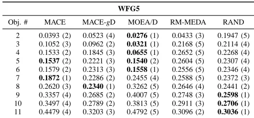
The main performance metric for the comparative studies in this work is the generational distance (GD) indicator. This metric has been chosen since we are mainly interested in the convergence properties of the studied algorithms.

• Generational Distance (GD), introduced in [60], is

de-fined thus:

D(A,P⋆_{) =}

P

s∈A

min_{kP⋆

1−sk2, . . . ,kPN⋆ −sk2}

|A_|

(32) where _|P⋆_| is the cardinality of the set _P⋆. The GD metric measures the distance of the elements in the set A from the nearest point of the reference PF. A is an approximation of the true Pareto front and _P⋆ is the reference Pareto optimal set.

B. Experiment Description

In Section III, it was explained that the three objectives that MOEAs have to achieve – namely convergence, diversity and PF coverage – can be reduced to only one, convergence, in the generalized decomposition framework. Therefore, the most important quantity of interest becomes some measure of convergence to the PF. For this reason, the GD metric was used, see (32).

The problem set chosen to perform the experiments is the WFG toolkit [28], specifically problems WFG2–WFG9, since they contain several challenging problems, are scalable and the PFs are known a priori. For all test instances we used

32 decision variables and the k parameter is calculated as: k= 4 + 2_·(M₋1), the only exception being the2-objective instances of the test problems where it is set to 4; M is the number of objectives. The neighbourhood sizeT in MOEA/D was selected to be 10% of the population size N, since, according to [12], this appears to be a setting producing good results for MAPs. The population size was the same for all the algorithms, see Table II. The parameters of the CE method are the same in MACE and MACE-gD and have been selected according to the suggestions in [47], see Table III. Lastly, the reference Pareto fronts used in MACE-gD to produce the

optimal weighting vectors for the test instances WFG2 and

WFG3 were generated by a random sample of the true Pareto set and, for the problems WFG4–WFG9, the method described in Appendix A was employed for generating a concave Pareto optimal set.

In practice such information is usually not available before the application of the optimization algorithm. This problem can be addressed using an identification method to determine the PF shape during the optimization; the methodology to be adopted will be investigated in future research.

Finally, as is probably evident from the selection of the reference PF for the generation of the weighting vectors in MACE-gD, we assume that the DM is interested in a PF that is uniformly distributed on that front. This is due to several considerations. First, if we follow the method usually applied in MOEA benchmarking for generating the reference PF of concave geometry, say for 3 dimensions, i.e. generate a set of evenly distributed weighting vectors and then project onto the first octant of the unit sphere, then for higher dimensions, due to the curvature of the hypersphere this will induce a large bias in the reference set. Namely, the density of Pareto optimal solutions will be higher near the edges of the PF compared to the density near the centre. Conversely, to produce a truly even distribution of Pareto optimal solutions in high dimensions is still an unresolved issue for an arbitrary number of points, even for PFs that have simple geometry, see [44], [45].

C. Experiment Results

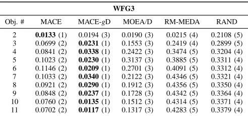
A summary of the GD-metric performance of the algorithms is presented in Tables IV–XI. The values in bold indicate the best performing algorithm for the particular instance of a test problem. We used the Kruskal-Wallis test at the 95%

confidence level to verify whether the mean performance of the studied algorithms is different. For each algorithm and for each problem instance we used the Wilcoxon two-sided rank sum test for α = 0.05 (95% confidence level). Every time an algorithm outperforms another in the test group, for a test instance, a 1 was added to its rank. Since we have 5

algorithms, the maximum rank for an algorithm is 4. A rank of4means that the algorithm in question performs better than all other algorithms for that particular test instance. In the case that no algorithm is clearly better we have a tie thus both algorithms are displayed in bold in Table IV–Table XI. An algorithm with a rank of 4 is denoted with a (1), one with a rank of 3 with a (2) and so forth, with (1) denoting the best performing algorithm and(5)the worst performer. These values are recorded to the right of the GD-metric performance in Tables IV–XI.

Table IV presents the results of the algorithms for 2–11

MACE-gD WFG2 f1 f2 f3 MACE WFG2 f1 f2 f3 MOEA/D WFG2 f1 f2 f3 RM-MEDA WFG2 f1 f2 f3 WFG3 f1 f2 f3 WFG3 f1 f2 f3 WFG3 f1 f2 f3 WFG3 f1 f2 f3 WFG4 f1 f2 f3 WFG4 f1 f2 f3 WFG4 f1 f2 f3 WFG4 f1 f2 f3 WFG5 f1 f2 f3 WFG5 f1 f2 f3 WFG5 f1 f2 f3 WFG5 f1 f2 f3 0 1 2 0 1 2 0 1 2 0 1 2 0 1 2 0 1 2 0 1 2 0 1 2 0 1 2 0 1 2 0 1 2 0 1 2 0 1 2 0 1 2 0 1 2 0 1 2 0 2 4 0 2 4 0 2 4 0 2 4 0 2 4 0 2 4 0 2 4 0 2 4 0 2 4 0 2 4 0 2 4 0 2 4 0 2 4 0 2 4 0 2 4 0 2 4 0 2 4 6 0 2 4 6 0 2 4 6 0 2 4 6 0 2 4 6 0 2 4 6 0 2 4 6 0 2 4 6 0 2 4 6 0 2 4 6 0 2 4 6 0 2 4 6 0 2 4 6 0 2 4 6 0 2 4 6 0 2 4 6

Fig. 5. MACE-gD, MACE, MOEA/D and RM-MEDA Pareto front for3-objective instances of the WFG2–WFG5 test problems.

TABLE IV

GD-METRIC PERFORMANCE OF THE STUDIED ALGORITHMS ON THE

WFG2PROBLEM FOR2–11OBJECTIVES.

WFG2

Obj. # MACE MACE-gD MOEA/D RM-MEDA RAND

2 0.0816 (3) 0.1027 (4) 0.0656 (2) 0.0279 (1) 0.1687 (5) 3 0.0353 (1) 0.0386 (2) 0.0444 (3) 0.0794 (4) 0.1929 (5) 4 0.0712 (2) 0.0485 (1) 0.1283 (4) 0.1274 (3) 0.1998 (5) 5 0.0718 (2) 0.0471 (1) 0.1717 (4) 0.1674 (3) 0.2125 (5) 6 0.0573 (2) 0.0423 (1) 0.1489 (3) 0.1979 (4) 0.2228 (5) 7 0.0650 (2) 0.0487 (1) 0.1081 (3) 0.2152 (4) 0.2335 (5) 8 0.0525 (2) 0.0379 (1) 0.0806 (3) 0.2434 (4) 0.2649 (5) 9 0.0471 (2) 0.0286 (1) 0.0791 (3) 0.2563 (4) 0.2638 (5) 10 0.0495 (2) 0.0168 (1) 0.0658 (3) 0.2694 (4) 0.2785 (5) 11 0.0453 (2) 0.0108 (1) 0.0814 (3) 0.2793 (4) 0.2867 (5)

TABLE V

GD-METRIC PERFORMANCE OF THE STUDIED ALGORITHMS ON THE

WFG3PROBLEM FOR2–11OBJECTIVES.

WFG3

Obj. # MACE MACE-gD MOEA/D RM-MEDA RAND

MACE-gD WFG6 f1 f2 f3 MACE WFG6 f1 f2 f3 MOEA/D WFG6 f1 f2 f3 RM-MEDA WFG6 f1 f2 f3 WFG7 f1 f2 f3 WFG7 f1 f2 f3 WFG7 f1 f2 f3 WFG7 f1 f2 f3 WFG8 f1 f2 f3 WFG8 f1 f2 f3 WFG8 f1 f2 f3 WFG8 f1 f2 f3 WFG9 f1 f2 f3 WFG9 f1 f2 f3 WFG9 f1 f2 f3 WFG9 f1 f2 f3 0 1 2 0 1 2 0 1 2 0 1 2 0 1 2 0 1 2 0 1 2 0 1 2 0 1 2 0 1 2 0 1 2 0 1 2 0 1 2 0 1 2 0 1 2 0 1 2 0 2 4 0 2 4 0 2 4 0 2 4 0 2 4 0 2 4 0 2 4 0 2 4 0 2 4 0 2 4 0 2 4 0 2 4 0 2 4 0 2 4 0 2 4 0 2 4 0 2 4 6 0 2 4 6 0 2 4 6 0 2 4 6 0 2 4 6 0 2 4 6 0 2 4 6 0 2 4 6 0 2 4 6 0 2 4 6 0 2 4 6 0 2 4 6 0 2 4 6 0 2 4 6 0 2 4 6 0 2 4 6

Fig. 6. MACE-gD, MACE, MOEA/D and RM-MEDA Pareto front for 3 objective instances of the WFG6–WFG9 test problems.

TABLE VI

GD-METRIC PERFORMANCE OF THE STUDIED ALGORITHMS ON THE

WFG4PROBLEM FOR2–11OBJECTIVES.

WFG4

Obj. # MACE MACE-gD MOEA/D RM-MEDA RAND

2 0.0345 (3) 0.0344 (3) 0.0211 (1) 0.0392 (4) 0.1161 (5) 3 0.0617 (3) 0.0522 (2) 0.0316 (1) 0.0939 (4) 0.1302 (5) 4 0.0749 (3) 0.0740 (2) 0.0655 (1) 0.1336 (4) 0.1358 (5) 5 0.1438 (3) 0.1048 (1) 0.1653 (5) 0.1464 (4) 0.1407 (2) 6 0.1358 (1) 0.1414 (2) 0.1959 (5) 0.1668 (4) 0.1549 (3) 7 0.2349 (4) 0.1997 (3) 0.2739 (5) 0.1898 (2) 0.1770 (1)

8 0.3176 (4) 0.2351 (3) 0.3371 (5) 0.2172 (2) 0.2025 (1)

9 0.3995 (5) 0.3028 (3) 0.3958 (4) 0.2495 (1) 0.2568 (2) 10 0.3791 (4) 0.3265 (3) 0.4001 (5) 0.2718 (2) 0.2577 (1)

11 0.4839 (5) 0.3875 (3) 0.4644 (4) 0.3162 (1) 0.3540 (2)

TABLE VII

GD-METRIC PERFORMANCE OF THE STUDIED ALGORITHMS ON THE

WFG5PROBLEM FOR2–11OBJECTIVES.

WFG5

Obj. # MACE MACE-gD MOEA/D RM-MEDA RAND

2 0.0393 (2) 0.0523 (4) 0.0276 (1) 0.0433 (3) 0.1947 (5) 3 0.1052 (3) 0.0962 (2) 0.0321 (1) 0.2168 (5) 0.2114 (4) 4 0.1533 (2) 0.1845 (3) 0.0655 (1) 0.2652 (5) 0.2268 (4) 5 0.1537 (2) 0.2221 (3) 0.1540 (2) 0.2604 (5) 0.2307 (4) 6 0.1579 (2) 0.2313 (3) 0.1558 (1) 0.2556 (5) 0.2346 (4) 7 0.1872 (1) 0.2286 (2) 0.2455 (4) 0.2588 (5) 0.2372 (3) 8 0.2620 (3) 0.2340 (1) 0.3262 (5) 0.2646 (4) 0.2441 (2) 9 0.3357 (4) 0.2685 (2) 0.4007 (5) 0.2748 (3) 0.2598 (1)

10 0.3497 (4) 0.2789 (2) 0.3813 (5) 0.2911 (3) 0.2706 (1)