Delaunay graph mapping based mesh deformation for simulation of a spanwise rigid and flexible flapping NACA0012 wing using DES with parallel implementation

(1)

Delaunay graph mapping based mesh deformation for

simulation of a spanwise rigid and flexible flapping

NACA0012 wing using DES with parallel

implementation

Naveed Durrani1and Sajid Raza Chaudhry2

National Engineering and Scientific Commission, Islamabad, Pakistan

and

Ning Qin.3

Department of Mechanical Engineering, University of Sheffield, UK

A flapping NACA0012 wing with spanwise rigid and flexible configurations is simulated using the Delaunay graph mapping based mesh deformation technique. This mesh deformation scheme is quite efficient and gives a good alternate to the spring analogy due to its non-iterative nature and simple implementation. It is also well suited for the parallel implementation due to its preservation of the original mesh topology.

The preliminary simulated case is spanwise rigid at Garrick frequency of 1.82 and Reynolds number 30,000, corresponding to the experimental data by Heathcote et. al [AIAA-2006-2870]. The results obtained for this case are in a good agreement with the experimental data for the instantaneous thrust. The simulation also predicts the lag in flapping motion cycle and generated thrust due to the dynamic effects of the flapping cycle and a corresponding phase lag is depicted in the thrust during the flapping cycle. The detailed paper will also include the implementation and results of the spanwise flexible flapping NACA0012 wing.

Nomenclature

A = surface area

d

C

= drag coefficient

DES

C

= model constant taken as 0.65

CT = instantaneous coefficient of thrust

d = wall distance, length scale for turbulence model

dA = differential surface area

F = inviscid flux vector

f = shedding frequency

KG = Garrick Frequency

G = viscous flux vector

n = normal area vector

P, p = pressure

Pr = prandtl number

q = heat flux

Q = primitive variables vector

Re = Reynolds number

1

PhD, AIAA Member, E-mail [email protected] 2

PhD, AIAA Member

49th AIAA Aerospace Sciences Meeting including the New Horizons Forum and Aerospace Exposition

4 - 7 January 2011, Orlando, Florida

AIAA 2011-1266

(2)

Sr = Strouhal number (

shedding frequency (f) * characteristic length (c)

freestream velocity (Uinf)

)

t

= temporal symbol representing time

T = temperature

u, v, and w = cartesian velocity components

u

= instantaneous velocity

u

= averaged velocity

Uinf = free stream velocity

V = volume

W = conserved variables vector

X = position vector in x, y and z direction

g

&

= spatial vector related with grid

/ /

x y z

&

= direction vector along x,y and z axis

t

&

= the time domain

J

= ratio of specific heats

ī

= preconditioning matrix

T

P

= turbulent or eddy viscosity

T

Q

= kinematic eddy viscosity

Q

= modified kinematic eddy viscosity

U

= density

p

U

=

p

U

w

at constant temperature

T

U

=

T

U

w

at constant pressure

ij

W

ª º

¬ ¼

Ĳ

= stress tensor

W

= pseudo time

w

W

= wall shear stress

K

= span wise location

ALE = Arbitrary Lagrangian Eulerian

CFD = Computational Fluid Dynamics

CFL = Courant–Friedrichs–Lewy condition

DES = Detached Eddy Simulation

DG-DES = Dynamic Grid-Detached Eddy Simulation (Sheffield University Code)

GCL = Geometric Conservation Law

GIS = Grid Induced Separation

LES = Large Eddy Simulation

MPI = Message Passing Interface

NS = Navier-Stokes

RANS = Reynolds Averaged Navier Stokes Equations

S-A = Spalart-Allmaras turbulence model

SGS = Sub-grid-scale

URANS = Unsteady RANS

(3)

I. Introduction

He Flapping wing aerodynamics is presently an active area of research both in CFD and in experimental domain. However, it is a challenge to move the mesh for three dimensions for flapping motion. The preliminary simulated case is spanwise rigid at Garrick frequency of 1.82 and Reynolds number 30,000, corresponding to the experimental data of Ref. [1]. A history of pitching and plunging airfoils can be traversed from Ref. [2 -16]. Spring analogy becomes computationally expensive due to its iterative nature. Delaunay graph based grid deformation scheme[17]is a non iterative and powerful method for mesh motion and offers a good alternate to the traditional spring analogy.

II. Numerical Scheme

A parallel, density based unstructured solver called Dynamic Grid Detached-Eddy Simulation(DG-DES)[18,19] is used for the present study. The code solves the unsteady Reynolds Averaged Navier-Stokes (RANS) equations using dual-time stepping approach. The governing equations are discretized using a cell-centered finite volume method. The convective terms are discretized using the Roe scheme[20]. A single equations Spalart-Almaras turbulence model[21]is used for the Detached-Eddy simulation formulation. For domain decomposition, an open source code Metis[22]is used. Further details can be found in Ref. [18] and Ref. [19].

A. Governing equations

The governing Naver-Stokes equations are presented below:

N

inviscid flux

Conservative variables viscous flux

.

0

V A

dV

d

t

_w

ª

º

w

_«

_»

w

³³³

W

³³

_¬

F

G

_¼

A

(1) where primitive variable matrix Q is presented as,

p

u

v

w

T

§ ·

¨ ¸

© ¹

Q

,

u

v

w

E

U

½

°

®

¾

°

¯

¿

W

and

x y z

§

· ¨

¸

¨ ¸

¨

¸

©

¹

F

, x y z

§

· ¨

¸

¨ ¸

¨

¸

©

¹

G

(2)

T

(4)

B. Dual-time stepping

The main structure of the in-house code DG-DES used for the present study is presented in Chart 1.

Chart 1: Flow chart showing the structure of dual-time stepping for moving mesh

t 't t

W W 'W

Backward Euler scheme for physical time advancement

x Residual calculation with Fluxes calculated using Roe Flux Difference splitting

x 3/4 stage explicit Runge Kutta scheme for pseudo time advancement using specified CFL number with local time stepping.

x Update conservative variables

Maximum Physical time steps reached Pseudo time block

Yes

No Yes

No

Move mesh

Converged Or

Maximum Pseudo iterations reached

START

Specify total number of: x physical time steps x pseudo time steps per

physical time iteration

Periodic Storing of results

W WWW 'W

x Residual calculation with Fluxes calculated using Roe Flux Difference splitting

x 3/4 stage explicit Runge Kutta scheme for pseudo time advancement using specified CFL number with local time stepping.

x Update conservative variables

Pseudo time block

No

Converged Or

Maximum Pseudo iterations reached

END

(5)

C. Moving mesh with arbitrary Lagrangian-Eulerian (ALE) formulation

A previous study by the authors[23] used the ALE formulation to simulate the flapping teardrop element with flexible tail. ALE are a set of equations representing Eulerian, Lagrangian or any intermediate stage field. Historically, the ALE has been widely applied in fluid and structural dynamics with deforming domain. General inviscid Eulerian formulation can be represented as:

0 t

w

W

F

X

(3)

Where,

X

xi

ˆ

yj

ˆ

zk

ˆ

Following the Eulerian system of equations is written to describe the mean flow properties, in integral Cartesian form for an arbitrary control volume V with differential surface area dA.

.

0

V A

dV

d

t

_w

w

³³³

W

³³

F A

(4)

u

v

w

E

U

½

°

®

¾

°

¯

¿

W

x y z

§

· ¨

¸

¨ ¸

¨

¸

©

¹

F

x

u

uu

p

uv

uw

uE

pu

U

½

°

®

¾

°

¯

¿

F

, _y

v

vu

vv

p

vw

vE

pv

U

½

°

®

¾

°

¯

¿

F

, _z

w

wu

wv

ww

p

wE

pw

U

½

°

®

¾

°

¯

¿

F

It is clear that the inviscid terms comprise convection and pressure terms.

1

0

1

0

x

Convective terms Pressure terms

u

uu

p

u

p

uv

v

uw

w

uE

pu

E

u

U

½

°

° °

°

° °

°

° °

®

¾

® ¾

°

° °

°

° °

°

° °

¯

¿

¯ ¿

F

(5) 1 0 0 1 0 y

v

vu u

v p

vv p v

vw w

vE pv E v

U

½ ½ ½

° ° ° ° ° °

® ¾ ® ¾ ® ¾

° ° ° ° ° ° ° ° ° ° ° ° ° ° ° ° ° ° ¯ ¿ ¯ ¿ ¯ ¿ F

(6)

1

0

1

z

w

wu

u

w

p

wv

v

ww

p

w

wE

pw

E

w

U

½

°

° °

°

° °

°

° °

®

¾

® ¾

°

° °

°

° °

°

° °

¯

¿

¯ ¿

F

The word “arbitrary” in ALE indicates that it could be both “Lagrangian” and ”Eulerian” or anywhere in between them. Therefore, the control volume

V t

( )

and the control area

w

A t

( )

are the function of time now. For the velocity of the moving control surface

w

A t

( )

as

v

_g, where

g g g g

u

v

w

ª º

« »

¬ ¼

v

,

The resulting ALE formulation becomes:

( ) ( )

.

0

V t A t

dV

d

t

_w

w

³³³

W

³³

F A

(6)

1

0

1 (

)

0

x g

u

u u

v

p

w

E

u

U

½

° °

_{® ¾}

° °

¯ ¿

F

1

0

0 (

)

1

0

y g

u

v v

v

p

w

E

v

U

½

° °

_{® ¾}

° °

¯ ¿

F

(7)

1

0

0 (

)

0

1

z g

u

w w

v

p

w

E

w

U

½

° °

_{® ¾}

° °

¯ ¿

F

By replacing these inviscid terms with the inviscid flux terms of NS equations, the complete set of NS equations for ALE formulation is obtained.

(7)

D. Oscillating NACA0012 Wing

Delaunay Graph Mapping based mesh deformation [17]is an efficient non-iterative mesh deformation scheme. The domain mesh for NACA0012 wing is shown in “Fig. 1(a)”. The Delaunay graph is generated with selected input domain points as shown in “ Fig. 1(b)”. In order to display the Delaunay graph map, “Fig. 1(c)” presents the Delaunay triangulation on the base line mesh. The zoomed view of the wing is shown in “Fig. 1 (d)”.

The mesh statistics of the mesh used in this simulated are tabulated in ”Table 1”. It is structured mesh, generated in Gambit with near wall clustering. The number of Delaunay graph elements used for this mesh deformation is 4821. It is to be ensured that all the internal mesh nodes (excluding the boundary nodes) are encompassed by the Delaunay Graph elements. The mesh resolution especially in the LES region is less than what is generally adopted for the hybrid RANS-LES methodology.

Number of nodes

Number of

elements Nx ×Ny ×Nz

Type of cells

Brick Tetrahedral Pyramid

[image:7.612.85.535.142.500.2]

274533 255760 278x46x20 255760 0 0

Figure 1. Domain and Delaunay Graph meshes a) Mesh of the domain b) Delaunay Graph with the 3D mesh

c) Delaunay Graph only d) Zoom view of the wing

c)

d)

a)

b)

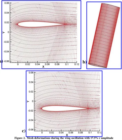
[image:7.612.83.530.641.680.2]

(8)

It is to be noticed that the overall mesh resolution is coarse as shown in Fig. 2. An open source code Metis[22]is used for the mesh partitioning for parallel computations.

As mentioned before, a coarse mesh is used initially to validate the mesh motion methodology and to speed up the results. Figure 2 (a) and (c) are two instantaneous mesh images at the top and bottom peak during the mesh motion. Figure 2 (b) presents the mesh over the surface of the NACA0012 wing.

E. Case details

The case simulated corresponds to the inflexible motion case as presented in the “Fig. 2”. However, the experimental inflexible case has a certain tip displacement due to the flexibility of the material. For the simulated case, the root and tip displacements are in zero phase lag (fully rigid body). “Table 2” presents the different

[image:8.612.89.516.140.629.2]

Figure 2. Mesh deformations during the wing oscillation with 17.5% c amplitude a) Top peak location b) 3D wing mesh c) Bottom peak location

a)

_b)

c)

(9)

parameters from the case set up for the numerical simulation and correspond to the experimental data[1]. The trajectory followed in this simulation is similar to the profile by the ‘Root’ as shown in Fig. 3.

Re = 30000

Scale 9.413196E-02

chord (m) 1

velocity (m/sec) 5

Density 1.17666

Viscosity 1.84602186E-05

Re 3.000000E+04

Gamma 1.4

R 287.04

T 300

C 347.212903

Meu 1.84602186E-05

P 101324.545920

Mach 0.014400

meu_ref 1.789400E-05

T_ref 288.150000

C 110.4

frequency (flapping) 30.771908

Amplitude (m) 0.016473093

distance traveled by le in

1sec (m) 2.03E+00

Garrick Freq (KG) 1.820000E+00

[image:9.612.167.470.97.347.2]

Strouhal Number (Sr) 0.202763397

Figure 3. Tip displacements as a function of time, Re=30,000, kG=1.82. Ref. [1]

[image:9.612.206.407.373.688.2]

(10)

F. Boundary conditions

The NACA0012 wing is assumed to be fully rigid. It means that the root and tip of the wing have same trajectory in the oscillation direction. Hence, the symmetry boundary conditions are applied on the both ends of the wing. The outer boundary is kept as a farfield boundary by neglecting the top and bottom wall of the water tunnel.

III. Results

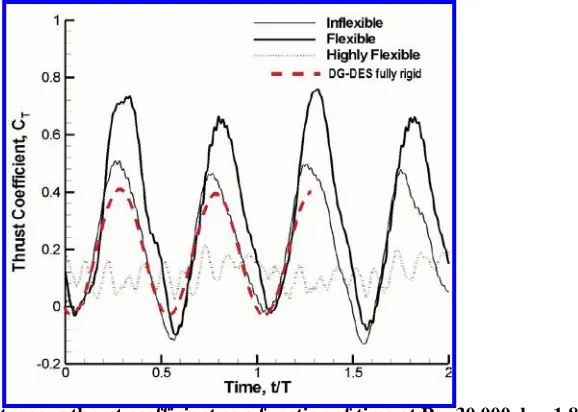
The results of instantaneous thrust coefficient for the stated case are presented along with the contours of static pressure

[image:10.612.192.481.169.375.2]

and vorticity magnitude for the flapping cycle. Figure 4 presents the instantaneous coefficient of thrust plots for the simulated NACA0012 wing with the experimental data. It is worth notice that the experimental data termed as ‘inflexible’ is closest to our simulated case which is also rigid and “inflexible”.

[image:10.612.170.446.436.667.2]

Figure 5 Coefficient of thrust plotted against non dimensional t/T Trajectory during flapping motion: Amplitude of motion (m) plotted against time(sec) Flowfield data at Pt1, Pt2, Pt3 and Pt4, represented by blue rectangles, is discussed below

Figure 4 Instantaneous thrust coefficient as a function of time at Re=30,000, kG=1.82.

(11)

The main difference is that although termed as the ‘inflexible’, this experimental wing still has some small degree of flexibility. This flexibility is obvious in figure 4 as a small difference between the motion profile of the root and tip.The result of the instantaneous thrust coefficient CTis quite encouraging. In fact, as presented in figure 4, the trajectory of Inflexible wing has tip displacement which may contribute to the generation of thrust for experimental inflexible wing.

The top side of the experimental setup is a free fluid surface which whereas the bottom is rigid water tank bed. This experimental setup is simulated by keeping the top and bottom of the domain as “Farfield” boundary conditions. So any ph ysical effects due to the free open side on the top or on the bottom are neglected. A much finer grid with lesser dissipation and better capability of the resolving and preserving the separated flow structures may give improved flowfield results.

The trajectory of the flapping motion and the coefficient of thrust are plotted in Figure 5. It is to be noticed that both have different time scales along x-axis. The arrows describe the direction of motion and the flowfiled results and mesh at marked points (Pt1-Pt4) are presented ahead.

[image:11.612.120.496.232.687.2]

(12)

[image:12.612.89.535.102.687.2]

The dynamic effects are clearly observable from the lag of both trajectory and the coefficient of thrust. It is in line with the physical and experimental observations where the flow dynamics has a dynamic effect due to the momentum of the fluid.

Figure 7. Line contour plots of vorticity magnitude. Flowfield description at Pt1, Pt2, Pt3 and Pt4 (from top to bottom)

(13)

The vector plot in Fig. 6 coloured with velocity magnitude show the dynamics of the flow at different locations from Pt1 to Pt4 as defined in Fig. 5. The sharp variations at the leading and trailing edge of the wing make it essential to have a proper mesh resolution in these regions for better capturing of the flow physics. These plots are taken from the cross section of the flapping wing at the mid-span location. Pt1 to Pt4 presented in Fig. 7, show the vorticity line contours at different locations along the trajectory. The effect of mesh motion and hence the related dynamic effect is clearly visible during the motion cycle. Another aspect observed that apparently the effect of downstream turbulence is not very significant in this case and a relatively very coarse mesh has generated encouraging results.

The Delaunay graph based mesh deformation used in this scheme has been very efficient and its non-iterative nature has made the mesh deformation for massively large computations possible.

IV. Conclusions

The Delaunay graph based mesh deformation scheme is successfully implemented in the serial and MPI version of DG-DES solver[23,24]. The results presented are for the spanwise rigid NACA0012 wing. No appreciable bottle neck or reduction in efficiency is observed in the solution due the deforming mesh simulation. The master node does the mesh deformation and calculates the new mesh parameters during the time slot when it is otherwise idle (for non-moving meshes) and waiting for the slave nodes to pass on the convergence data. The speed and the quality of the deformed mesh are quite good. The simulation of spanwise flexible wing is to be done in the same way. However, for this study, only spanwise rigid wing is simulated as a test case. It is observed that particularly for the three dimensional Delaunay graph based mesh deformation[25] is sensitive to the quality of the parent Delaunay triangles. The resulting mesh may deteriorate with the number of iteration if the area ratios are calculated at each step of the mesh motion from the highly skewed parent Delaunay triangles. In this study, the preference is given to use the mesh area ratios calculated from the un-deformed mesh, corresponding to the original graph. It reduces the computational time considerably by avoiding the calculation of the area ratios at each step of mesh deformation. It also ensures that the subsequent skewness in the Delaunay triangles has a minimal effect on the resulting mesh quality. However, it reduces the flexibility of this methodology. If the original Delaunay graph fails to provide the feasible mesh for the complete cycle, it is still preferred to generate another Delaunay graph after some specified number of simulation iterations instead of each mesh deformation step. The number of these steps has to be decided after observing the step during which the mesh deformation fails. Obviously, if a single Delaunay Graph suffices the complete mesh motion, the mesh deformation becomes very fast. The Delaunay elements generated at the first step are not to be generated again and their connectivity remains the same. It is to function much faster than the original Delaunay Graph that needs to be computed at each mesh deformation step. The flexibility and accuracy of the mesh deformation increases with the increase in the number of Delaunay triangles generated at extra computational cost.

It is to be noted that this simulation does not cover the effect of wall region near the tip of the NACA0012 wing as in the experimental setup. In the experimental setup, the clearance between the wing tip and the floor of the water tunnel is 5c/3 which corresponds to the 56% of the semi span. The effect of wall may have significant impact on the experimental data. The mesh used in this simulation is very coarse and the grid resolution in the LES region is very coarse as well. For a better hybrid RANS-LES simulation, the mesh size is to be considerably increased to be able to capture the unsteady separated flow physics properly.

The results obtained for the instantaneous coefficient of thrust are quite encouraging in comparison with the experimental data. It imbibes the confidence in using moving meshes with Detached-Eddy simulation with encouraging results. Due to its simplicity and non-iterative nature, the Delaunay-Graph mesh deformation methodology can be extended to LES simulations with massive mesh sizes, especially for huge size grids that cannot afford iterative mesh deformation scheme.

Further simulations for spanwise flexible and rigid configuration are underway and will be included in the future work.

Acknowledgments

The authors thankfully acknowledge the computational time on Bluegrid and Greengrid clusters at the University of Sheffield, UK for this research. The support from National Engineering and Scientific Commission (NESCOM), Pakistan is acknowledged. The first author was funded by the overseas research scholarship (ORS) from the University of Sheffield and is gratefully acknowledged.

(14)

2

Knoller, R., “Die Gesetze des Luftwiderstandes,” Flug und Motortechnik (Wien), Vol. 3, No. 21, pp. 1–7, 1909. 3

Katzmayr, R., “Effect of Periodic Changes of Angle of Attack on Behavior of Airfoils,” NACA Rept. 147, Oct. 1922 (translated from Zeitschrift fuer Flugtechnik und Motorluftschiffahrt, March 31, 1922, pp. 80–82, and April 13, pp. 95–101) , 1922.

4

Theodorsen, T., “General Theory of Aerodynamic Instability and the Mechanism of Flutter”, NACA, TR-496, 1935. 5

Garrick, I. E., “Propulsionof a Flapping and Oscillating Airfoil,”NACA Rept. 567, 1936. 6

Von Karman, T., and Burgers, J. M., “General Aerodynamic Theory-Perfect Fluids,” Aerodynamic Theory, edited by W. F. Durand, Division E, Vol. 2, Julius–Springer, Berlin, 1943.

7

Silverstein, A., and Joyner, U. T., “Experimental Verification of the Theory of Oscillating Airfoils,” NACA Report 673, 1939.

8

Bratt, J. B., “Flow Patterns in the Wake of an Oscillating Airfoil,” Aeronautical Research Council, R&M 2773,March 1950. 9

Freymuth, P., “Propulsive Vortical Signature of Plunging and Pitching Airfoils,” AIAA Journal, Vol. 26, No. 7, pp. 881-883, 1988.

10

Koochesfahani, M.M., “Vortical Patterns in the Wake of an Oscillating Airfoil,” AIAA Journal, Vol. 27, No. 9, pp. 1200-1205, 1989.

11

Dohring, C.M., Platzer, M.F., Jones, K.D. and Tuncer, I.H., “Computational and Experimental Investigation of the Wakes Shed From Flapping Airfoils and Their Wake Interference/Impingement Characteristics, “Characterisation and Modification of Wakes from Lifting Vehicles in Fluids, Vol. 33, pp. 1-9, 1996.

12

Lai, J.C.S. and Platzer, M.F., “Jet Characteristics of a Plunging Airfoil,” AIAA Journal, Vol. 37, No. 12, pp. 1529-1537, 1999.

13

Katz, J., and Weihs, D., “Hydrodynamic Propulsion by Large Amplitude Oscillation of an Airfoil with Chordwise Flexibility,” Journal of Fluid Mechanics, Vol. 88, No. 3, pp. 485–497, 1978.

14

Murray, M. M., and Howle, L. E., “Spring Stiffness Influence on an Oscillating Propulsor,” Journal of Fluids and Structures, Vol. 17, No. 7, pp. 915–926, 2003.

15_{Isaac, K.M., Colozza, A. and Rolwes, J., “Force Measurements on a Flapping and Pitching Wing at Low Reynolds} Numbers,” AIAA paper 2006-450, 44th AIAA Aerospace Sciences Meeting and Exhibit, Reno, Nevada, 9-12 January 2006.

16_{Heathcote, S. and Gursul, I., “Flexible Flapping Airfoil Propulsion at Low Reynolds Numbers,” AIAA Journal, vol. 45, No.} 5, pp. 1066-1079, 2007.

17

X. Liu, N. Qin, and H. Xia, “Fast Dynamic Grid Deformation Based on Delaunay Graph Mapping“, Journal of Computational Physics, 211(2):405–423, 2005.

18

N. I. Durrani, “Hybrid RANS-LES Simulations for Separated Flows Using Dynamic Grids”, Ph.. D. thesis, University of Sheffield, UK, March 2009.

19

N. Qin and H. Xia, “Detached eddy simulation of a synthetic jet for flow control”, Proceedings of the Institution of Mechanical Engineers, Part I: Journal of Systems and Control Engineering, Vol. 222, No. 5, pp. 373-380.

20

P. L. Roe, “Approximate Riemann Solvers, Parameters Vectors and Difference Schemes“, Journal of Computational Physics, 43:357–372, 1981.

21

P. R. Spalart and S. R. Allmaras, “A One-Equation Turbulence Model for Aerodynamic Flows“, AIAA Paper 92-0439, January 1992.

22

G. Karypis and V. Kumar, “User Manual of METIS: A Software Package for Partitioning Unstructured Graphs, Partitioning Meshes and Computing Fill-Reduced Orderings of Sparse Matrices, Version 4.0“, University of Minnesota, 1998.

23

Durrani N. and Qin N., “Numerical Simulation of Flexible Flapping Airfoil Propulsion using Dynamic Mesh at Low Reynolds Numbers“, AIAA 2008-64, 46th AIAA Aerospace Sciences Meeting and Exhibit. Reno, Nevada, 7-10 January 2008.

24

P. D. Thomas and C. K. Lombard, “Geometric Conservation Law and its Applications to Flow Computations on Moving Grids“, AIAA Journal, 17:1030–1037, 1979.

25

C.W. Hirt, A. A. Amsden, and J.L. Cook. “An Arbitrary Lagrangian-Eulerian Computing Method for All Flow Speeds”. Journal of Computational Physics, 14(3):227-253, 1974 (reprinted in 1997)

26

Spalart, P. R., Jou W-H., Strelets M., Allmaras, S. R., “Comments on the Feasibility of LES for Wings and on a Hybrid RANS/LES Approach” Advances in DNS/LES, 1stAFOSR Int. Conf. on DNS/LES, Greyden Press, Columbus Oh, 4-8 August, 1997.

(15)

This article has been cited by:

1. Jiangtao Huang, Zhenghong Gao, Chao Wang. 2014. A new grid deformation technology with high quality and robustness based on quaternion. Chinese Journal of Aeronautics27, 1078-1085. [CrossRef]