A Forecasting Model Based On K-means Clustering And Time-invariant Fuzzy Relationship Groups

Vol. 2 Issue 8, August - 2016

A Forecasting Model Based on K-Means

Clustering and Time-Invariant Fuzzy

Relationship Groups

Thai Nguyen University of Technology, Thai Nguyen University

Thainguyen, Vietnam

Nguyen Cong Dieu

Institute of Information Technology, Viet nam Academy of Science and Technology

Hanoi, Vietnam

Nguyen Thi Huong

Thai Nguyen University of Technology, Thai Nguyen University Thainguyen, Vietnam

Abstract — In the past years, most of the fuzzy forecasting methods based on fuzzy time series used the static length of intervals, i.e., the same length of intervals. The drawback of the static length of intervals is that the historical data are roughly put into intervals, even if the variance of the historical data is not high. In this paper, an improved forecasting model is used to forecast the student enrolment at the University of Alabama. Firstly, a method of unequal-sized intervals partitioning based on K-means clustering algorithm is proposed. Secondly, used fuzzy logical relationship groups in determination of fuzzy relations stage to overcome the defect of traditional fuzzification method. Finally

,

Keywords— fuzzy relationship groups (FTS), forecasting, K-mean clustering(KM), enrollments.

I. INTRODUCTION

For more than one decade, many methods have been presented for fuzzy time series forecasting [1]-[2], [6], [7] either to find a better forecasting result or to do faster computations. The concept of fuzzy time series was proposed by Song and Chissom[1]-[3]. Ref. [1],[2] introduced fuzzy time series in two parts as time-variant and time-invariant. In this study, it has been focused on time-invariant fuzzy time series. Fuzzy time series forecasting models consist of three stages. All these stages play an active role on the forecasting performance. These stages are; fuzzification, determination of fuzzy relations and defuzzification, respectively. However, most of the existing fuzzy forecasting methods based on fuzzy time series used the static length of intervals, i.e., the same length of intervals such as [1],[2],[3],[9],[10]. The drawback of the static length of intervals is that the historical data are roughly put into the intervals, even if the variance of the

historical data is not high. Moreover, the forecasting accuracy rates of the existing fuzzy forecasting methods based on the static length of intervals are not good enough. Recently, Ref.[16] presented a new hybrid forecasting model which combined particle swarm optimization(PSO) with fuzzy time series to find proper length of each interval. Chen and Kao [19] proposed a method of partitioning the uni-verse of discourse in which PSO algorithm is exploited to find optimal unequal-sized intervals according to the distribution of historical data of time series. In [20] also utilized PSO algorithm to construct unequal-sized intervals for developing Type-2 fuzzy model of stock time series on basis of the scheme of supervised learning. These the universe of discourse partitioning methods based on unequal-sized intervals are used to forecast enrollments, stock index, etc. Additionally, in [17] proposed a new method to forecast enrolments based on automatic clustering techniques and fuzzy logical relationships. In this paper, a forecasting model based on two computational methods, K-mean clustering technique and fuzzy logical relationship groups Firstly, we use the K-mean clustering algorithm to divide the historical data into clusters and adjust them into intervals with different lengths. Then, based on the new intervals, we fuzzify all the historical data of the enrolments of the University of Alabama and calculate the forecasted output by the proposed method. Compared to the other methods existing in literature, particularly to the first-order fuzzy time series, the proposed method showed a better accuracy in forecasting the number of students in enrolments of the University of Alabama.

The rest of this paper is organized as follows. In Section II, we briefly review some concepts of fuzzy time series and K-mean clustering are given. In Section III, we presented forecasting model based on the K-means clustering algorithm and time-invariant fuzzy logical relationship groups. Then, the computational results are shown and analyzed in Section IV. The conclusions are discussed in Section V.

II. FUZZY TIME SERIES AND K-MEANS ALGORITHM

Vol. 2 Issue 8, August - 2016 A. Fuzzy Time Series

In [1], [2], Song et al. proposed the definition of fuzzy time series based on fuzzy sets [18]. Let U={u1,u2,…,un

} be an universal set; a fuzzy set A of U is defined as

A={ fA(u1)/u1+…+fA(un)/un }, where fA is a membership function of a given set A, fA :U [0,1], fA(ui) indicates the grade of membership of uiin the fuzzy set A, fA(ui) ϵ [0, 1], and 1≤ i ≤ n . General definitions of fuzzy time series are given as follows:

Definition 1: Fuzzy time series

Let Y(t) (t = ..., 0, 1, 2 …), a subset of R, be the universe

of discourse on which fuzzy sets fi(t) (i = 1,2…) are defined and if F(t) be a collection of fi(t)) (i = 1, 2…). Then, F(t) is called a fuzzy time series on Y(t) (t . . ., 0, 1,2, . . .).

Definition 2: Time-invariant fuzzy time series

Let F(t) be a fuzzy time series. If for any time t, F(t) = F(t - 1) and F(t) only has finite elements, then F(t) is called a time-invariant fuzzy time series. Otherwise, it is called a time-variant fuzzy time series.

Definition 3: Fuzzy logic relationship

If there exists a fuzzy relationship R(t-1,t), such that F(t) = F(t-1)R(t-1,t), where " " is an arithmetic operator, then F(t) is said to be caused by F(t-1). The relationship between F(t) and 1) can be denoted by F(t-1)→ F(t). Let Ai = F(t) and Aj = F(t-1), the relationship between F(t) and F(t -1) is denoted by fuzzy logical relationship Ai→ Aj where Ai and Aj refer to the current state or the left hand side and the next state or the right-hand side of fuzzy time series.

Definition 4: 𝝀- order fuzzy time series

Let F(t) be a fuzzy time series. If F(t) is caused by F(t-1), F(t-2),…, F(t-𝜆+1) F(t-𝜆) then this fuzzy relationship is represented by by F(t-𝜆), …, F(t-2), F(t-1)→ F(t) and is called an 𝝀- order fuzzy time series.

Definition 5: Fuzzy Relationship Group (FLRG)

Fuzzy logical relationships in the training datasets with the same fuzzy set on the left-hand-side can be further grouped into a fuzzy logical relationship groups. Suppose there are relationships such that

𝐴_𝑖 → 𝐴_𝑗

𝐴_𝑖 → 𝐴_𝑘 …….

So, based on Chen[3] , these fuzzy logical relationship can be grouped into the same FLRG as : 𝐴_𝑖 → 𝐴_𝑗 , 𝐴_𝑘…

B. K-means clustering technique

The K-means algorithm is simple, straightforward and is based on the firm foundation of analysis of variances. It clusters a group of data vectors into a predefined number of clusters. It starts with randomly initial cluster centroids and keeps reassigning the data objects in the dataset to cluster centroids based on the similarity between the data object and the cluster centroid. The reassignment procedure will not stop until a convergence criterion is met (e.g., the fixed iteration number, or the cluster result does not change after a certain number of iterations). The main idea of the K-means algorithm is the minimization of an objective function usually taken up as a function of the deviations

between all patterns from their respective cluster centers [5].

The K-means algorithm can be summarized as:

1. Randomly select cluster centroid vectors to set an initial dataset partition.

2. Assign each document vector to the closest cluster centroids.

3. Recalculate the cluster centroid vector 𝑐𝑗using

equation (1).

𝑐𝑗= 1

𝑛𝑗∑∀𝑑𝑗∈𝑠𝑗𝑑𝑗 (1)

4. Repeate step 2 and 3 until the convergence is achieved.

where dj denotes the document vectors that belong to cluster Sj; cj stands for the centroid vector; nj is the number of document vectors that belong to cluster Sj

III. FORECASTING MODEL BASED ON FRGS-KM

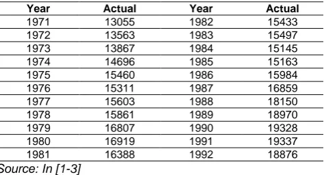
An improved hybrid model for forecasting the enrolments of University of Alabama (named FRGs-KM) based on Time – invariant Fuzzy Relationship Groups and K-Means clustering techniques. At first, we apply K-means clustering technique to classify the collected data into clusters and adjust these clusters into contiguous intervals for generating intervals from numerical data then, based on the interval defined, we fuzzify on the historical data determine fuzzy relationship and create fuzzy relationship groups; and finally, we obtain the forecasting output based on the fuzzy relationship groups and rules of forecasting are our proposed. The historical data of enrolments of the University of Alabama are listed inTable 1.

TABLE I: HISTORICAL DATA OF ENROLMENTS

Year Actual Year Actual

1971 13055 1982 15433

1972 13563 1983 15497

1973 13867 1984 15145

1974 14696 1985 15163

1975 15460 1986 15984

1976 15311 1987 16859

1977 15603 1988 18150

1978 15861 1989 18970

1979 16807 1990 19328

1980 16919 1991 19337

1981 16388 1992 18876

Source: In [1-3]

A. A Clustering Algorithm For Creating Intervals From Historical Data Of Enrolments.

The algorithm composed of 4 steps is introduced step-by-step with the same dataset.

Step 1: Apply the K-means clustering algorithm to partition the historical time series data into p clusters and sort the data in clusters in an ascending sequence. in this paper, we set p=14 clusters, the results are as follows:

Vol. 2 Issue 8, August - 2016

Step 2: Create the cluster center and adjust the clusters into intervals.

In this step, we use automatic clustering techniques [17] to generate cluster center (Centerj) from clusters in step 1 according to (2).

𝑪𝒆𝒏𝒕𝒆𝒓_𝒋=∑ di n i=1

n (2)

where di is a datum in Clusterj , n denotes the number of data in Clusterj and 1 ≤ 𝑗 ≤ 𝑝.

Then, Adjust the clusters into intervals according to the follow rules. Assume that Centerk and Centerk+1 are adjacent cluster centers, then the upper bound Uboundj of clusterjand the lower bound Lboundk+1 of clusterj+1 can be calculated according to (3) and (4) as follows:

𝑈𝑏𝑜𝑢𝑛𝑑_𝑘=𝐶𝑒𝑛𝑡𝑒𝑟𝑘+ 𝐶𝑒𝑛𝑡𝑒𝑟𝑘+1

2 (3)

𝐿𝑏𝑜𝑢𝑛𝑑𝑘+1= 𝐶𝑙𝑢𝑠𝑡𝑒𝑟_𝑈𝐵𝑘 (4) where k=1,...,p-1. Because there is no previous cluster before the first cluster and there is no next cluster after the last cluster, the lower bound Lbound1 of the first cluster and the upper bound Uboundpof the last cluster can be calculated according to (5) and (6) as follows:

𝐿𝑏𝑜𝑢𝑛𝑑₁= 𝑪𝒆𝒏𝒕𝒆𝒓_𝟏− (𝑪𝒆𝒏𝒕𝒆𝒓_𝟏− 𝐶𝑙𝑢𝑠𝑡𝑒𝑟_𝑈𝐵₁) (5)

𝑈𝑏𝑜𝑢𝑛𝑑_𝑝= 𝑪𝒆𝒏𝒕𝒆𝒓_𝒑+ (𝑪𝒆𝒏𝒕𝒆𝒓_𝒑− 𝐶𝑙𝑢𝑠𝑡𝑒𝑟_𝐿𝐵_𝑝) (6) From (2), (3), (4), (5) and (6), we get cluster centers are shown in Table 2.

TABLE II:GENERATE CLUSTER CENTER FROM CLUSTERS

No Clusters Center Lbound Ubound

1 {13055, 13563} 13309 13030 13588

2 {13867} 13867 13588 14434

3 {14696, 15145, 15163} 15001 14434 15156

4 {15311} 15311 15156 15387

5 {15460, 15433, 15497} 15463 15387 15533

6 {15603} 15603 15533 15762.5

7 {15861, 15984} 15922 15762.5 16155

8 {16388} 16388 16155 16597.5

9 {16807} 16807 16597.5 16833

10 {16859} 16859 16833 16889

11 {16919} 16919 16889 17534.5

12 {18150} 18150 17534.5 18536.5

13 {18970, 18876} 18923 18536.5 19127.5

14 {19328, 19337} 19332 19127.5 19536.5

Step 3: Let each cluster Clusterj form an interval intervalj, which means that the upper bound Uboundj and the lower bound Cluster_Lboundj of the cluster clusterj are also the upper bound interval_Uboundj and the lower bound interval_Lboundj of the interval intervalj, respectively. Calculate the middle value Mid_valuej of the interval intervalj according to (7) shown in Table 3:

𝑀𝑖𝑑_𝑣𝑎𝑙𝑢𝑒𝑗=

𝑖𝑛𝑡𝑒𝑟𝑣𝑎𝑙_𝐿𝑏𝑜𝑢𝑛𝑑𝑗+ 𝑖𝑛𝑡𝑒𝑟𝑣𝑎𝑙_𝑈𝑏𝑜𝑢𝑛𝑑𝑗

2 (7) where interval_Uboundj and interval_Lboundj are the upper bound and the lower bound of intervalj, respectively, and j = 1,…,p.

TABLE III:THE MIDPOINT OF EACH INTERVAL UJ(1 ≤ 𝑗 ≤ 14)

No Intervals Mj = Midpoint intevals

1 (13030, 13588] 13309

2 (13588, 14434] 14011

3 (14434, 15156] 14795

4 (15156, 15387] 15271.5

5 (15387, 15533] 15460

6 (15533, 15762] 15647.5

7 (15762, 16155] 15958.5

8 (16155, 16598] 16376.5

9 (16598, 16833] 16715.5

10 (16833, 16889] 16861

11 (16889, 17534] 17211.5

12 (17534, 18536] 18035

13 (18536, 19128] 18832

14 (19128, 19536] 19332

B. Enrolment Forecasting model Using Fuzzy Relationship Groups And K-Mean Algorithm

In this section, we present a new method for forecasting enrolments based on the K-mean clustering algorithm and time –invariant fuzzy logical relationships group. The proposed method is now presented as follows:

Step 1: Partition the universe of discourse into intervals After applying the procedure K-mean clustering, we can get the following 14 intervals and calculate the middle value of the intervals are listed in Table 3.

Step 2: Fuzzify all historical data.

Define each fuzzy set 𝐴𝑖based on the new obtained 14 intervals in step 1 and the historical enrolments shown in Table 1. For 14 intervals, there are 14 linguistic variables Ai (1≤ 𝑖 ≤ 14). For example, 𝐴₁＝{very very very very few }, 𝐴₂＝{very very very few}, 𝐴₃＝{very very few}, 𝐴4 ＝{very few }, 𝐴5 ＝{few }, 6 ＝ {moderate}, 𝐴₇＝{many}, 𝐴₈＝{many many}, 𝐴₉＝{very many}, 𝐴10＝{too many}, 𝐴11＝{too many many}, 𝐴12＝ {too many many many}, 𝐴₁₃＝{too many many many many} and 𝐴14＝{too many many many many many}. Each linguistic variable represents a fuzzy set such that the according to (8). Each historical value is fuzzified according to its highest degree of membership. If the highest degree of belongingness of a certain historical time variable, say F(t−1) occurs at fuzzy set Ai, then

F(t−1) is fuzzified as Ai

A₁ = 1

𝑢1+

0.5 𝑢2+

0

𝑢3+ ⋯ +

0 𝑢14

A₂ =0.5

𝑢1+

1 𝑢2+

0.5

𝑢3+ ⋯ +

0 𝑢14

---

A14 =

0 𝑢₁+

0

𝑢₂+ ⋯ +

0.5 𝑢₁₃+

1 𝑢₁₄

For simplicity, the membership values of fuzzy set A_i

either are 0, 0.5 or 1, where1 ≤ i ≤ 14. The value 0, 0.5 and 1 indicate the grade of membership of uj in the fuzzy set Ai.

The way to fuzzify a historical data is to find the interval it belongs to and assign the corresponding linguistic value to it and finding out the degree of each data belonging to each A_i . If the maximum membership of the historical data is under Ai , then the fuzzified historical data is labeled as A_i.

For example, the historical enrolment of year 1973 is 13867 which falls within u2 = (13588, 14282], so it belongs to interval u2 Based on Eq. (8), Since the highest membership degree of u2 occurs at A2 is 1, the historical time variable F(1973) is fuzzified as A2. The results of fuzzification are listed in Table 4, where all historical data are fuzzified to be fuzzy sets.

Vol. 2 Issue 8, August - 2016 TABLE IV: FUZZIFIED ENROLMENTS OF THE UNIVERSITY OF ALABAMA

Year

Actual data

Fuzzy

set Year

Actual data

Fuzzy set

1971 13055 A1 1982 15433 A5

1972 13563 A1 1983 15497 A5

1973 13867 A2 1984 15145 A3

1974 14696 A3 1985 15163 A4

1975 15460 A5 1986 15984 A7

1976 15311 A4 1987 16859 A10

1977 15603 A6 1988 18150 A12

1978 15861 A7 1989 18970 A13

1979 16807 A9 1990 19328 A14

1980 16919 A11 1991 19337 A14

1981 16388 A8 1992 18876 A13

Let Y(t) be a historical data time series on year t. The purpose of Step 1 is to get a fuzzy time series F(t) on Y(t). Each element of Y(t) is an integer with respect to the actual enrollment. But each element of F(t) is a linguistic value (i.e. a fuzzy set) with respect to the corresponding element of Y(t). For example, in Table 4, Y(1971) = 13055 and F(1971) = A1; Y(1973) = 13867 and F(1973) = A2; Y(1975) = 15460 and F(1975) = A5 and so on.

Step 3: Create all fuzzy logical relationships

Relationships are identified from the fuzzified historical data. So, from Table 4and base on Definition 3, we get first – order fuzzy logical relationships are shown in Table 5. where the fuzzy logical relationship 𝐴𝑖 → 𝐴𝑘 means "If the enrollment of year i is 𝐴_𝑖, then that of year i + 1 is 𝐴𝑘", where 𝐴𝑖 is called the current state of the enrollment, and 𝐴𝑘 is called the next state of the enrollment.

TABLE V: THE FIRST-ORDER FUZZY LOGICAL RELATIONSHIPS

No Relationships No Relationships

1 A1 -> A1 11 A8 -> A5

2 A1 -> A2 12 A5 -> A5

3 A2 -> A3 13 A5 -> A3

4 A3 -> A5 14 A3 -> A4

5 A5 -> A4 15 A4 -> A7

6 A4 -> A6 16 A7 -> A10

7 A6 -> A7 17 A10 -> A12

8 A7 -> A9 18 A12 -> A13

9 A9 -> A11 19 A13 -> A14

10 A11 -> A8 20 A14 -> A14

21 A14 -> A13

Step 4: Establish and calculate the forecasting values for all fuzzy logical relationship groups

By Chen [3], all the fuzzy relationship having the same fuzzy set on the left-hand side or the same current state can be put together into one fuzzy relationship group. Thus, from Table 5 and based on Definition 5, we can obtain 14 fuzzy logical relationship groups and compute the forecasted output for these groups according to (9 ) and (10) are listed in Table 6.

TABLE VI:FUZZY LOGICAL RELATIONSHIP GROUPS (FLRGS) Number of Groups FLRGs Forecasted value

1 A1 -> A1, A2 13660

2 A2 -> A3 14795

3 A3 -> A5, A4 15365.8 4 A5 -> A4, A5, A3 15175.5

5 A4 -> A6, A7 15803

6 A6 -> A7 15958.5

7 A7 -> A9, A10 16788.2

8 A9 -> A11 17211.5

9 A11 -> A8 16376.5

10 A8 -> A5 15460

11 A10 -> A12 18035

12 A12 -> A13 18832

13 A13 -> A14 19332

14 A14 -> A14, A13 19082

Calculate the forecasted output at time t by using the following principles:

Principle 1: If the fuzzified enrolment of year t-1 is Aj and there is only one fuzzy logical relationship in the fuzzy logical relationship group whose current state is Aj, shown as follows: A_j→ A_k ;then the forecasted enrolment of year t forecasted = mk (9) where mk is the midpoint of the interval uk and the maximum membership value of the fuzzy set Ak occurs at the interval uk

Principle 2: If the fuzzified enrolment of year t -1 is Aj and there are the following fuzzy logical relationship group whose current state is Aj , shown as follows:

Aj→ Ai1, Ai2, Aip

then the forecasted enrolment of year t is calculated as

follows: f𝑜𝑟𝑒𝑐𝑎𝑠𝑡𝑒𝑑 =∑ 𝑚𝑖𝑘

𝑝 𝑘=1

𝑝 (10) where 𝑚𝑖1, 𝑚𝑖2 , 𝑚𝑖𝑘 are the middle values of the intervals ui1 , ui2 and uik respectively, and the maximum membership values of Ai1, Ai2 , . .. ,Aik occur at intervals ui1 , ui2, uik , respectively.

Step 5: Generate all fuzzy forecasting rules

Based on each group of fuzzy relationships created and relative forecasting values in Step 4, we can generate corresponding fuzzy forecasting rules. The if-then statements are used as the basic format for the fuzzy forecasting rules. Assume a first-order fuzzy forecasting rule R_i is ‘‘if x = A, then y = B’’, the if-part of the rule ‘‘x = A’’ is termed antecedent and the then-part of the rule ‘‘y = B’’ is termed consequent. For example, if we want to forecast enrolments Y(t) using fuzzy group 1 for the first-order fuzzy time series in Table 6, the fuzzy forecasting rule R₁ is will be ‘‘if 𝐹(𝑡 − 1) = 𝐴1

then Y(t) = 13660.

For example, Table 7demonstrates the 14 fuzzy rules generated by the first-order fuzzy groups of Table 6. In the same way, we can get the 14 fuzzy rules based on the first-order fuzzy relationship groups, as shown in Table 7.

TABLE VII: THE FUZZY IF-THEN RULES OF THE FIRST-ORDER FUZZY RELATIONSHIPS ON ENROLMENTS.

Rules Antecedent Consequent

1 If F(t-1)==A1 Then Y(t) =13660

2 If F(t-1)==A2 Then Y(t) =14795

3 If F(t-1)==A3 Then Y(t) =15365.8

4 If F(t-1)==A4 Then Y(t) =15175.5

5 If F(t-1)==A5 Then Y(t) =15803

6 If F(t-1)==A6 Then Y(t) =15958.5

7 If F(t-1)==A7 Then Y(t) =16788.2

8 If F(t-1)==A8 Then Y(t) =117211.5

9 If F(t-1)==A9 Then Y(t) =16376.5

Vol. 2 Issue 8, August - 2016

13 If F(t-1)==A13 Then Y(t) =19212 14 If F(t-1)==A14 Then Y(t) =18995.2

Step 6: forecasting output based on the forecast rules After the forecast rules are created, we can use them to forecast the training data. Suppose we want to forecast the data Y(t), we need to find out a matched forecast rule and get the forecasted value from this rule. If we use the first-order forecast rules listed in Table 6to forecast the data Y(t), we just simply find out the corresponding linguistic values of F(t-1) with respect to the data Y(t-1) and then compare them to the matching parts of all forecast rules. Suppose a matching part of a forecast rule is matched, we then get a forecasted value from the forecasting part of this matched forecast rule. For example, if we want to forecast the data Y(1975), it is necessary to find out the corresponding linguistic values of F(1974) with respect to Y(1974). We then have the following pattern. If F(1974) == A3 then forecast Y(1975) = 15365.8 . In the same way, we complete forecasted results based on the first - order fuzzy forecast rules in Table 7 are listed in Table 8.

TABLE VIII: FORECASTED ENROLMENTS OF UNIVERSITY OF ALABAMA

BASED ON THE FIRST – ORDER FUZZY TIME SERIES.

Year Actual Fuzzified Results

1971 13055 A1 Not forecasted

1972 13563 A1 13660

1973 13867 A2 13660

1974 14696 A3 14795

1975 15460 A5 15365.8

1976 15311 A4 15175.5

1977 15603 A6 15803

1978 15861 A7 15958.5

1979 16807 A9 16788

1980 16919 A11 17211.5

1981 16388 A8 16376.5

1982 15433 A5 15460

1983 15497 A5 15175.5

1984 15145 A3 15175.5

1985 15163 A4 15365.8

1986 15984 A7 15803

1987 16859 A10 16788

1988 18150 A12 18035

1989 18970 A13 18832

1990 19328 A14 19332

1991 19337 A14 19082

1992 18876 A13 19082

To calculate the forecasted performance of proposed method in the fuzzy time series, the mean square error (MSE) and the mean absolute percentage error (MAPE) are used as an evaluation criterion to represent the forecasted accuracy. The MSE value and MAPE value are computed according to (11) and (12) as follows:

MSE = 1

n∑ (Fi− Ri) 2 n

i=1 (11)

𝑀𝐴𝑃𝐸 = 1

𝑛∑ | 𝐹𝑖−𝑅𝑖

𝑅𝑖 |

𝑛

𝑖=1 ∗ 100% (12) Where, Ri notes actual data on year i, Fi forecasted value on year i, n is number of the forecasted data

IV. EXPERIMENTAL RESULTS

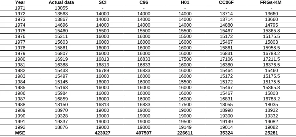
Experimental results for FRGs-KM will be compared with the existing methods, such as the SCI model [2], the C96 model[3], the H01 model[6] and CC06F model [11] by using the enrolment of Alabama University from 1972s to 1992s are listed in Table 9 .

Table 9shows a comparison of MSE and MAPE of our method using the first-order fuzzy time series under number of intervals=14, where MSE and MAPE are calculated according to (11) and (12) as follows:

𝑀𝑆𝐸 = ∑21𝑖=1(𝐹𝑖−𝑅𝑖)2

𝑁 =

(13660−13563)2+(13660−13867)2…+(19082−18876)2

21 = 25281.43

𝑀𝐴𝑃𝐸 = 1

21∑ | 𝐹𝑖−𝑅𝑖

𝑅𝑖 |

21

𝑖=1 ∗ 100% = 1 21(

𝑎𝑏𝑠(13600−13563) 13563 +

⋯ +𝑎𝑏𝑠(19082−18876)

18876 ) =0.79%

where N denotes the number of forecasted data, Fi denotes the forecasted value at time i and Ri denotes the actual value at time i.

TABLE IX: A COMPARISON OF THE FORECASTED RESULTS OF FRGS-KM WITH THE EXISTING MODELS BASED ON THE FIRST-ORDER FUZZY TIME SERIES

UNDER DIFFERENT NUMBER OF INTERVALS.

Year Actual data SCI C96 H01 CC06F FRGs-KM

1971 13055 - - - - -

1972 13563 14000 14000 14000 13714 13660

1973 13867 14000 14000 14000 13714 13660

1974 14696 14000 14000 14000 14880 14795

1975 15460 15500 15500 15500 15467 15365.8

1976 15311 16000 16000 15500 15172 15175.5

1977 15603 16000 16000 16000 15467 15803

1978 15861 16000 16000 16000 15861 15958.5

1979 16807 16000 16000 16000 16831 16788.2

1980 16919 16813 16833 17500 17106 17211.5

1981 16388 16813 16833 16000 16380 16376.5

1982 15433 16789 16833 16000 15464 15460

1983 15497 16000 16000 16000 15172 15175.5

1984 15145 16000 16000 15500 15172 15175.5

1985 15163 16000 16000 16000 15467 15365.8

1986 15984 16000 16000 16000 15467 15803

1987 16859 16000 16000 16000 16831 16788.2

1988 18150 16813 16833 17500 18055 18035

1989 18970 19000 19000 19000 18998 18932

1990 19328 19000 19000 19000 19300 19332

1991 19337 19000 19000 19500 19149 19082

1992 18876 19000 19000 19149 19014 19082

Vol. 2 Issue 8, August - 2016

MAPE 3.22% 3.11% 2.66% 0.81% 0.79%

From Table 9, we can see that the FRGs-KM has a smaller MSE and MAPE than SCI model [2] the C96 model [3], the H01 model [6] and the CC06F model [11]. To verify the forecasting effectiveness for

high-order FLRs, the C02 model [9] is used to compare with the proposed model. From Table 10, The FRGs-KM model gets the lowest MSE value of 20896 for the 8th-order FLRGs and The average MSE value is 35861 smaller than the C02 model.

TABLE X: A COMPARISON OF THE FORECASTED ACCURACY BETWEEN OUR PROPOSED METHOD AND C02 MODEL, THE CC06F MODEL FOR SEVEN

INTERVALS WITH DIFFERENT NUMBER OF ODERS

Methods Number of oders

2 3 4 5 6 7 8 9 Average(MSE)

C02 model 89093 86694 89376 94539 98215 104056 102179 102789 95868

FRGs-KM 80802 35767 27493 28141 29351 28269 20896 32231 35368.75

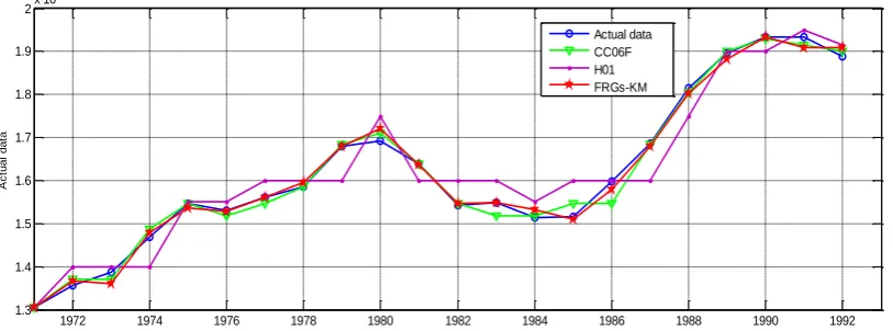
Displays the forecasting results of H01 model, CC06F model and FRGs-KM. The trend in forecasting of enrolment by first-order of the fuzzy time series in

comparison to the actual enrolment can be visualized in Fig.1.

Fig. 1: The curves of the H01, CC06F models and FRGs-KM for forecasting enrolments of University of Alabama

From Fig.1, the graphical comparison clearly shows that the forecasting accuracy of the proposed model is more precise than those of existing models with different first-order fuzzy logical relation.

V. CONCLUSION

In this paper, we have presented a hybrid forecasting method (named FRGs-KM) in the first-order fuzzy time series model based on the time-invariant fuzzy logical relationship groups and K-means clustering techniques. In this method, we tried to classify the historical data of Alabama University into clusters by K-means techniques and then, adjust the clusters into intervals with different lengths. In case study, we have applied the proposed method to forecast the number of students enrolling in the University of Alabama from 1972s to 1992s. The simulation result showed that the proposed method is able to obtain the forecasted value with better accuracy compared to other methods existing in literature. The detail of comparison was presented in Table 9, Table 10 and Fig.1.

Although this study shows the superior forecasting capability compared with existing forecasting models; but the proposed model is a new forecasting model and only tested by the enrolment data. To assess the effectiveness of the forecasting model, there are two suggestions for future research. The first, we use more

intelligent methods (e.g., particle swarm optimization, ant colony or a neural network) to deal with forecasting problems. The second, we will decide to use multi factor forecasting based on the described scheme to deal with more complicated real-world problems for decision-making such as weather forecast, crop production, stock markets, and etc. That will be the future work of this research.

ACKNOWLEDGMENT

The work reported in this paper has been supported by Thai Nguyen University of Technology - Thai Nguyen University.

REFERENCES

[1] Q. Song, B.S. Chissom, “Forecasting Enrollments with Fuzzy Time Series – Part I,” Fuzzy set and system, vol. 54, pp. 1-9, 1993b.

[2] Q. Song, B.S. Chissom, “Forecasting Enrollments with Fuzzy Time Series – Part II,” Fuzzy set and system, vol. 62, pp. 1-8, 1994.

[3] S.M. Chen, “Forecasting Enrollments based on Fuzzy Time Series,” Fuzzy set and system, vol. 81, pp. 311-319. 1996.

[4] Hwang, J. R., Chen, S. M., & Lee, C. H. “Handling forecasting problems using fuzzy time series”. Fuzzy Sets and Systems, 100(1–3), 217–228, 1998.

1972 1974 1976 1978 1980 1982 1984 1986 1988 1990 1992

1.3 1.4 1.5 1.6 1.7 1.8 1.9

2x 10

4

Years

A

c

tu

a

l

d

a

ta

Vol. 2 Issue 8, August - 2016 [5] Michael K. Ng, “A note on constrained k-means

algorithms,” Pattern Recognition, vol. 13, pp. 515-519, 2000.

[6] Huarng, K. “Heuristic models of fuzzy time series for forecasting”. Fuzzy Sets and Systems, 123, 369–386, 2001b .

[7] Singh, S. R. A simple method of forecasting based on fuzzytime series. Applied Mathematics and Computation, 186, 330–339, 2007a.

[8] Singh, S. R. A robust method of forecasting based on fuzzy time series. Applied Mathematics and Computation, 188, 472–484, 2007b.

[9] S. M. Chen, “Forecasting enrollments based on high-order fuzzy time series”, Cybernetics and Systems: An International Journal, vol. 33, pp. 1-16, 2002.

[10] H.K.. Yu “Weighted fuzzy time series models for TAIEX forecasting ”, Physica A, 349 , pp. 609–624, 2005.

[11] Chen, S.-M., Chung, N.-Y.“Forecasting enrollments of students by using fuzzy time series and genetic algorithms”. International Journal of Information and Management Sciences 17, 1–17, 2006a.

[12] Chen, S.M., Chung, N.Y.“Forecasting enrolments using high-order fuzzy time series and genetic algorithms”. International of Intelligent Systems 21, 485–501, 2006b.

[13] Lee, L.-W., Wang, L.-H., & Chen, S.-M. Temperature prediction and TAIFEX forecasting based

on fuzzy logical relationships and genetic algorithms. Expert Systems with Applications, 33, 539–550, 2007.

[14] Jilani, T.A., Burney, S.M.A. “A refined fuzzy time series model for stock market forecasting”. Physica A 387, 2857–2862. 2008.

[15] Wang, N.-Y, & Chen, S.-M. “Temperature prediction and TAIFEX forecasting based on automatic clustering techniques and two-factors high-order fuzzy time series”. Expert Systems with Applications, 36, 2143–2154, 2009.

[16] Kuo, I. H., Horng, S.-J., Kao, T.-W., Lin, T.-L., Lee, C.-L., & Pan. “An improved method for forecasting enrollments based on fuzzy time series and particle swarm optimization”. Expert Systems with applications, 36, 6108–6117, 2009a.

[17] S.-M. Chen, K. Tanuwijaya, “ Fuzzy forecasting based on high-order fuzzy logical relationships and automatic clustering techniques”, Expert Systems with Applications 38 ,15425–15437, 2011.

[18] Zadeh, L. A. Fuzzy sets. Information and Control, 8: 338-353, 1965.

[19] S.M. Chen, P.Y. Kao, TAIEX forecasting based on fuzzy time series, particle swarm optimization techniques and support vector machines, Inf. Sci. 247, 62-71, 2013.