A timeband framework for modelling real-time systems

White Rose Research Online URL for this paper:

http://eprints.whiterose.ac.uk/10929/

Version: Submitted Version

Article:

Burns, A. orcid.org/0000-0001-5621-8816 and Hayes, I.J. (2010) A timeband framework for

modelling real-time systems. Real-Time Systems. pp. 106-142. ISSN 1573-1383

https://doi.org/10.1007/s11241-010-9094-5

eprints@whiterose.ac.uk https://eprints.whiterose.ac.uk/

Reuse

Items deposited in White Rose Research Online are protected by copyright, with all rights reserved unless indicated otherwise. They may be downloaded and/or printed for private study, or other acts as permitted by national copyright laws. The publisher or other rights holders may allow further reproduction and re-use of the full text version. This is indicated by the licence information on the White Rose Research Online record for the item.

Takedown

If you consider content in White Rose Research Online to be in breach of UK law, please notify us by

White Rose Research Online

eprints@whiterose.ac.uk

Universities of Leeds, Sheffield and York

http://eprints.whiterose.ac.uk/

This is an author produced version of a paper published in

REAL-TIME SYSTEMS

White Rose Research Online URL for this paper:

http://eprints.whiterose.ac.uk/

10929

Published paper

Burns A, Hayes IJ

(2010)

Title: A timeband framework for modelling real-time systems

45 (1-2) 106-142

(will be inserted by the editor)

A Timeband Framework for Modelling Real-Time Systems

Alan Burns _· Ian J. Hayes

March 25, 2010

Abstract Complex real-time systems must integrate physical processes with digital control, human operation and organisational structures. New scientific foundations are required for specifying, designing and implementing these systems. One key chal-lenge is to cope with the wide range of time scales and dynamics inherent in such systems. To exploit the unique properties of time, with the aim of producing more dependable computer-based systems, it is desirable to explicitly identify distinct time bands in which the system is situated. Such a framework enables the temporal prop-erties and associated dynamic behaviour of existing systems to be described and the requirements for new or modified systems to be specified. A system model based on a finite set of distinct time bands is motivated and developed in this paper.

1 Introduction

The construction of large socio-technical real-time systems, such as those envisaged in cyber-physical applications, imposes a number of significant challenges, both tech-nical and organisational. Their complexity makes all stages of their development (re-quirements analysis, specification, design, implementation, deployment and mainte-nance/evolution) subject to failure and costly re-working. Even the production of an unambiguous behavioural description of an existing system is far from straightfor-ward.

One characteristic of these computer-based systems is that they are required to function at many different time scales (from microseconds or less to days or more). Time is clearly a crucial notion in the specification (or behavioural description) of computer-based systems, but it is usually represented, in modelling schemes for ex-ample, as a single flat physical phenomenon. Such an abstraction fails to support the

A. Burns

Department of Computer Science, University of York, UK.

I.J. Hayes

structural properties of the system, forces different temporal notions on to the same flat description, and fails to support the separation of concerns that the different time scales of the system facilitate. Even with a single time scale, system architects seem to have great difficulty in specifying temporal properties in anything other than very concrete implementation-level terms. But just as the functional properties of a system can be modelled at different levels of abstraction or detail, so too should its temporal properties be representable in different, but provably consistent, time scales.

To make better use of ‘time’, with the aim of producing more dependable computer-based systems, we propose a framework that explicitly identifies a number of distinct time bandsin which the system under study is situated. The framework enables the temporal properties of existing systems to be described and the requirements for new or modified systems to be specified.

In the following section we motivate the main notions and properties of the time-band framework. Then, in Section 3, an abstract model of timetime-bands is presented, and in Section 4 is extended to describe state. Section 5 gives a brief summary of the model. The model is, in itself, not intended to be a complete semantic description. That is achieved by ‘embedding’ the model in a parent notation/logic. The focus of this paper is, however, the timeband framework. Section 6 introduces some notation to allow specification of properties in the timeband framework. A short example of the use of the framework in presented in Section 7. Related and future work is dis-cussed in Section 8 and conclusions are covered in Section 9.

2 Motivation

A large real-time system exhibits dynamic behaviour on many different levels. The computational components have circuits that have nanosecond speeds, faster elec-tronic subcomponents and slower functional units. Communication on a fast bus is at the microsecond level but may be tens of milliseconds on slow or wide-area me-dia. Human time scales move from the 1ms neuron firing time to simple cognitive actions that range from 100ms to 10 seconds or more. Higher rational actions take minutes and even hours. Indeed it takes on the order of 1000 hours to become an ex-pert at a skilled task, such as flying a plane [45] and the development of highly skilful behaviour may take many years. At the organisational and social level, time scales range from a few minutes, through days, months and even years. Perhaps for some environmentally sensitive systems, consequences of failure may endure for centuries. To move from nanoseconds to centuries requires a framework with considerable de-scriptive and analytical power.

The concept of timebands comes from a detailed study of existing computer-based systems1 _{and their requirements (eg.[29]), ethnographical studies (eg. [7, 2]),}

the work of Newell [39] in his attempts to describe human cognition, work on system structure such as that of Simon [47], reports on system failures (eg. Columbus [5]), studies from areas such as the psychology and sociology of time [19, 22, 44, 34, 3], formalisms such as the teleo-reactive programming model [40, 41] and Statecharts

that require instantaneous state changes, and the few examples of modelling work that do attempt to consider more than one time scale within a system (eg. Corsettiet al[17, 13]).

As the concept of ‘now’ (present moment) seems to be fundamental to our rea-soning about time, it follows that notions such as ‘instantaneous’, ‘simultaneous’ and ‘immediate’ are natural ones to use in specifying temporal properties. As Bergada`a [3] states in his work on a temporal framework:

The present time could be made of moments that enable the allocation of time to different activities. They could also be made of duration in which the activity will take the time necessary for its completion.

From such observations and the literature noted above we distil the following properties that we identify as being of relevance to the modelling of complex real-time systems.

– The dynamics of a system (how quickly things change) are central to understand-ing its behaviour.

– Systems clearly operate at many different granularities (of time), ie. there are different abstract views of the dynamics of the system.

– It is useful to consider certain actions (events) as atomic and instantaneous (whilst allowing them to have internal state and behaviour at a more detailed level of description).

– It is useful to consider two or more events as occurring simultaneously (instanta-neously), or the response to some event being immediate (whilst allowing them to be separated in time at a more detailed level of description).

– The order (but not necessarily the time) at which events occur is important; prece-dence can give rise to causality.

– The durations of certain actions are important, but the measuring of time must not be overly precise and must allow for tolerance (non-determinacy) in the temporal domain.

– Abstract clocks are useful for relating and coordinating activities, but real clocks are never perfectly reliable or accurate.

– At each level of temporal behaviour it is useful to have access to both continuous and discrete notions of time – controlling actions are typically described using discrete time, the controlled object due to its continuously changing nature often requires dense time for its behavioural description.

– Hierarchical control (cascade control) and hierarchical scheduling (planning) are often observed through the time levels of a system.

– At each level of temporal behaviour similar phenomena are observed (e.g., cyclic/ repetitive actions, deadline-driven actions, synchronous and asynchronous event handling, agreement, coordination, etc.)

In the timebands framework, apparently more natural (and essentially atempo-ral) notions are available such as ‘immediate’, ‘instantaneous’, ‘simultaneous’, ’defi-nitely’ and ‘possible’. And durations are first expressed in general terms - for exam-ple “this is a minute-level activity” (ie. it will last a few minutes, rather than hours or seconds). Orders of magnitude between rates of change give an initial decomposi-tion of the system. Indeed the framework uses time itself to separate concerns in any architectural description or system specification.

The central notion in the framework is that of a time band that is defined by a granularity(eg. 1 minute) and a precision(eg. 5 seconds). Granularity defines the unit of time of the band; precision bounds the actual duration of an event that is deemed to be instantaneous in this band.

A system is assumed to consist not of a single time dimension but a finite set of bands. System activities are placed in some band B if they engage in significant events at the time scale represented by B, ie. they have dynamics that give rise to changes that are observable or meaningful in band B’s granularity. So, for example, at the 10 millisecond band, neural circuits are firing, significant computational functions are completing, and an amount of data communication will occur. At the 5 minute band, work shifts are changing, meetings are starting, etc. For any system there will be a highest and lowest band that gives a temporal system boundary – although there will always be the potential for larger and smaller bands. Note that at higher bands the physical system boundary may well be extended to include wider (and slower) entities such as legislative constraints or supply chain changes. To complete this short moti-vation section the important topics of sampling and rates of change are addressed.

Sampling. Our focus is on embedded real-time systems and hence we cannot avoid issues like sampling of inputs, and discretization of continuous quantities. For exam-ple, assume two proximity conditions are represented by boolean variablestopand bottom, representing that a controlled gate is at the top or bottom, respectively, of its travel. It is an error for the two proximity sensors to give simultaneous positive inputs. By placing this requirement for error detection in the minute band (with precision of 5 seconds) the following constraints are derived

– If in any interval of duration five seconds, or more,top andbottomare perma-nently true then the error conditionmustbe identified.

– If in any interval of duration five seconds, or less,topandbottomare true for part of the interval then the error conditioncanbe identified. Note that the intervals over whichtopandbottom, respectively, hold don’t have to be the same, or even overlap.

This dual use ofmustandcancannot be eliminated. One may move the requirement between time bands to decrease the value of the precision parameter, but even in the lowest band in the system there is an inevitable non-determinacy because true perfectly simultaneous polling of the two sensors is not possible.

– and that this band must have a dense notion of time whilst the others can be dis-crete. Rather, within any band, many (perhaps most) entities will be discrete, but some may be continuous. So if the purpose of an automatic ‘plant watering’ system in a greenhouse is to aid the growth of plants in some controlled environment, the rate of growth of the crop per week or day may be significant (but not per second or millisecond).

Consider, for example, the maximum rate of flow of water from a piston-style pump. At a higher time band, this may be stated asr litres per time unit, but at a lower time band, there are two phases of the piston: one filling the cylinder, in which there is almost no flow of water out of the pump; and the other emptying the cylinder, during which the rate of flow of water out of the pump is about twicer.

The maximum rate of change of a state variable may be uniform between some pairs of time bands, but not between others. By uniform, we mean that the maximum rates of change are the same (although they will be expressed with respect to the granularity of their respective time bands). For example, with the piston pump the rate of flow is not uniform at the time band that distinguishes the filling and emptying phases of the cylinder, but between a pair of higher bands the rate of flow may be uniform. At a still higher pair of bands, we may be switching the pump on and off to control the rate of flow over a broader time base. Again the rate of flow won’t be uniform, but between still higher bands, which don’t distinguish the on and off phases, it may emerge to be uniform again.

The motivation for proposing this timeband framework is to simplify the spec-ification of complex systems, improve the dependability of deployed systems and reduce the cost of designing (and redesigning) such systems. It allows dynamic prop-erties to be partitioned but not isolated from each other.

3 Definition of the Timeband Model

From the above considerations, a timeband model has been developed2 _{that is}

de-scribed in this and the next section (with some illustrative small examples). The aim of a timeband model is to be an essential part of any complete system description. It enables the temporal properties of existing systems to be described and the require-ments for new or modified systems to be specified. The informal description of the framework is supported by a formal model expressed in the Z notation [48, 25].

The framework is developed in a number of stages that build up the full model. Some examples of how this model can be extended into a language for actual use in specifying systems is then given. The list of topics discussed in this section are: time bands, granularity and precision, events and classes of events, precedence, simultane-ous and immediate, activities, mappings between bands, durations, and clocks. The next section covers state-related aspects of the model: a less determined view of state, change-of-state events, mapping states, accuracy and rates of change.

3.1 Time bands

For our formal model, we take the set of time bands (B) as a primitive type. Both “⊑” and “⊏” are relations between bands, with “⊑” forming a partial ordering3_on

time bands. The type of a relation between bands is given asB ↔ B. A relation is equivalent to a set of pairs, ie.(B ↔ B) =P_{(B × B), where}PXstands forpower set ofX, (i.e., the set of all subsets ofX).

⊑ :partial order[B]

⊏ :B ↔ B

∀b1,b2 :B •(b1⊏b2⇔b1⊑b2∧b16=b2)

For example, we may have that

MinuteBand⊏DayBand⊏MonthBand

From a focus on some bandB, adjacent bandsAandC, whereC⊏B⊏A, can be identified. Slower (higher or coarser) bands (e.g.A) can be taken to be unchanging (essentially constant) for issues of concern toB. At the other extreme, behaviours in the faster (lower or finer) bands (e.g.C) are assumed to be instantaneous inB. The actual differences in granularity betweenA,BandCare not precisely defined (and indeed may depend on the bands themselves) but will typically be in the range 1/10th to 1/100th. When bands map on to hierarchies (structural or control) then activities in bandAcan be seen to constrain the dynamics of bandB, whereas those inCenableB to proceed in a timely fashion. The ability to relate behaviour at different time bands is one of the main properties of the framework.

As an example, consider a university lecture course. Here there are immedi-ately four bands to identify. The year band in which new courses and curriculum are planned, the weekly band in which lectures are scheduled, the minute band that allows each lecture to be structured, and the second band that can capture various in-teractions with the available technical support (eg. laptop response). Whilst giving a lecture, one can assume that the curriculum is stable (unchanging) and that the laptop reacts instantaneously to slide change requests. Systems that don’t respect some form of time band structure can become extremely complex and difficult to comprehend, e.g., changing the course syllabus while lecturing is likely to lead to great confusion. It is important to emphasise that the full behaviour of a system is not obtained by refining down to the lowest band or by projecting emergent behaviours up to the high-est band. Rather it is the amalgamation of all band descriptions – all have behaviours that may be needed in any assertion about the system as a whole.

3 _{Although in most systems the bands will be totally ordered, there are applications, perhaps in the}

3.2 Granularity and precision

For each band itsgranularity, representing the unit of time in that band, andprecision, representing the measure of accuracy of events within that band. They must both be expressed relative to a lower band. For example, the granularity of theMonthBand with respect to theDayBandmay have a granularity defined as follows:

Granularity(MonthBand,DayBand) ={28,29,30,31}

and the granularity of the DayBand with respect to theMinuteBand is defined as follows:

Granularity(DayBand,MinuteBand) ={1440},

because there are 24∗60 = 1440minutes in a day. Hence the granularity of the MonthBandwith respect to theDayBandis

Granularity(MonthBand,MinuteBand) =

{28∗1440,29∗1440,30∗1440,31∗1440}.

Note that this set is not contiguous. For ease of presentation we assume that standard units such as minutes, milliseconds, etc, are well defined. However not all time scales will give rise to time bands.

For a bandb1, its granularity will be defined with respect to all lower bands; hence the domain of the granularity function is all pairs of bands(b1,b2), such thatb2is lower thanb1. Ifb1is related to a lower bandb2, andb2tob3, then the granularity ofb1with respect tob3is the composition of the granularities ofb1with respect to b2andb2with respect tob3. The setN_{is the natural numbers and}N_{1is the non-zero}

natural numbers.Granularityis a partial function ( 7→) from pairs of time bands to a non-empty set (P

1) of non-zero natural numbers.

Granularity: (B × B) 7→P 1N1

dom(Granularity) ={b1,b2 :B |b2⊏b1} ∀b1,b2,b3 :B; g:N_1•b3⊏b2⊏b1⇒

g∈Granularity(b1,b3)⇔

(∃g1,g2 :N_1•g=g1∗g2∧

g1∈Granularity(b1,b2)∧g2∈Granularity(b2,b3))

Within a band, behaviour is defined usingevents(which are instantaneous), activ-ities(that have duration) andstate(both discrete and continuous). These are defined in later sections, but important here is the property that events are defined to be in-stantaneous. And two or more events may be defined to be simultaneous. A band’s precisionis a constraint on the duration of ‘instantaneous’ and ‘simultaneous’ when measured in a finer band. For example, if the precision of the hour band is defined to be one minute then two simultaneous events must occur within a minute of each other.

Precision: (B × B) 7→N₁

dom(Precision) ={b1,b2 :B |b2⊏b1} ∀b1,b2,b3 :B •b3⊏b2⊏b1⇒

Precision(b1,b3)≤Precision(b1,b2)∗min(Granularity(b2,b3))

The definition of precision enables the framework to be used effectively for re-quirements specification. A temporal requirement such as a deadline is band-specific; similarly the definition of a timing failure. For example, being one second late may be a crucial failure in a computing device, whereas on a human scale being one sec-ond late for a meeting is meaningless. The duration of an activity is also ‘imprecise’ (within the band). Stating that a job will take three months is assumed to mean plus or minus a couple of days. Of course the precision of a band can only be explored in a lower band.

Again with the lecturing example, assume the precision of the minute band is one second. The instantaneous ‘slide change’ event when mapped to a laptop activity in a lower band must have a duration of not more than one second.

A key aspect of the timeband framework is that certain entities are considered to be instantaneous, and that they are then mapped to actions that have duration in a more detailed description of the system. One means of achieving this property would be to give all such entities a distinct precision. However in constructing behaviours from collections of entities, composition is much more straightforward if the same notion of precision applies. Moreover, the property of being ‘instantaneous’ relates to the level of the temporal abstraction not to the event itself. Hence the timeband framework starts by defining the bands and then places entities into the bands. If the entity is instantaneous it is represented by an event; if it has duration then it is represented by an activity with a duration that is adequately expressed using the granularity of the chosen band. Hence ‘adequately’ means with sufficient (but not excessive) precision over the value of the defined duration.

As well as the system itself manifesting behaviour at many different time bands, the environment will exhibit dynamic behaviour at different granularities. The bands are therefore linked to the environment at the level determined by these dynamics. In many system abstractions it is useful to assume the environment is in some form of steady state. But this assumption is clearly false as the environment evolves, perhaps as a result of the deployment of the embedded system under development. By map-ping the rate of this evolutionary change to an appropriate (relatively slow) time band one can gain the advantage of the steady-state abstraction whilst not ignoring slower dynamics.

3.3 Classes of events/activities

C band:B name:String

The above is a Z schema: it defines a record typeCwith two fields,bandandname.

3.4 Events

By definition, all actions within a band have similar timing dynamics. Within a band, eventsare instantaneous, whileactivitiesmay have a non-zero duration. Events are a natural way of expressing change within a system. By first defining behaviours to be instantaneous, an abstract definition of their cause and effect can be given. Also, seemingly impossible specifications can be given clear semantics. For example, the change-of-state event to turn off a water pump (as used in the case study in Section 7) is an event that ideally is instantaneous at some level of abstraction but clearly must take time at a more detailed level of description (in a finer band).

In a particular behaviour, there may be any (countable) number of instances of events of a particular class, including zero. The set of instances of an event class within a behaviour are totally ordered by precedence (see below), and hence we can also assign a unique index to an event instance. An event instance, “event” for short, is characterised by its class (time band and name), and a natural number index,n, indicating that it is occurrencenof events of that class within a behaviour.

E class:C index:N

We use the notationc#ito stand for the event of classcthat has index numberi. The idea of indexing event instances comes from RTL [30]. We define a shorthand for the time band of an event.

band:E → B

∀e:E •band(e) =e.class.band

For a band,b,Events(b)defines the set of all events in that band.

Events:B →P_E

∀b:B •Events(b) ={e:E |band(e) =b}

3.5 Precedence

has completed”, “before the gate has fired”). The framework must therefore represent both precedence relations and temporal frames of reference.

There is a strong link between temporal order (i.e., time-stamped events and ac-tivities) and precedence relations. However, in this framework, we do not impose an equivalence between time and precedence. Due to issues of precision, time cannot be used to infer precedence unless the time interval between two events is sufficiently large in the band of interest.

Where bands are (at least partially) ordered by granularity, then order and hence potential causality is preserved as one moves from the finer to the coarser bands. However, order and hence causality are not necessarily maintained as one moves down through the bands. Where order is important then proof must be obtained by examining the inter-band relationships.

A precedence relation (¹) defines a partial ordering4

on the events. Only events in the same time band are related by the precedence relation. We use the operator ≺for strict precedence. A behaviour of a system will consist of a nonempty set of events,ev, ordered by precedence. The notation ( ¹ )stands for the precedence relation taken as a whole.

BehaviourEvents ev:P

1E

¹ :partial order[E]

≺ :E ↔ E

∀e,f :E •

(e¹f ⇒e∈ev∧f ∈ev∧band(e) =band(f))∧

(e≺f ⇔e¹f ∧e6=f)

∀c:C; i,j:N_•i<j∧c#j∈ev⇒c#i∈ev∧c#i≺c#j

The above Z schema declares a number of fields and constrains them to satisfy the predicate below the line. Note that we don’t insist that all pairs of events are related one way or the other, but if bothe¹f andf ¹e, because “¹” is a partial order we insist thate=f. For each class of events, event instances are sequentially numbered from zero. Hence, if there is an instance of an event with indexj, then there must be event instances of the same class for all indices less thanjand these instances must precede thejth instance.

3.6 Simultaneous and immediate

In the specification of a system, an event may cause a responseimmediately (instanta-neously) – meaning that at this band the response is within the precision of the band. This use of untimed notions helps eliminate the problem of over specifying require-ments that is known to lead to implementation difficulties [29]. For example consider the naturally specified requirement ‘when the fridge door opens the light must come

on immediately’; this apparently gives no scope for an implementation to incorpo-rate the necessary delays of switches, circuitry and the light’s own latency. Making the term ‘immediate’ band specific, enables a finer-granularity band to include the necessary delays, latencies and processing time that are needed to support the imme-diate behaviour at the higher band. This separation of concerns removes the need to add a precise deadline to the ‘light-on’ event. An explicit deadline (of say 8.5ms) is too concrete – rather the deadline is ‘the definition of immediate in this band’. Ob-viously being immediate in the hour band is not the same as being immediate in the microsecond band.

Two events may have a precedence relationship (eg. slide X before slide Y) but occur at the same time (same hour).

It follows from these observations that, in this framework, there is a difference between two events being simultaneous and being ‘at the same time’. The former is a much stronger statement. Here two simultaneous events (in band B say) must, when viewed from a finer band, be within the precision of band B. Whereas ‘at the same time’ only required the two events to occur within the granularity of band B. As the precision is typically 1/10th to 1/100th of the granularity, clearly events being simultaneous is a much tighter constraint.

Precedence gives rise to potential causality. If P is before Q then information could flow between them, indeed P may be the cause of Q. In the use of the frame-work for specification we will need to use the stronger notion of precedence to imply causality. For example, “when the fridge door opens the light must come on”. Within the band of human experience this can be taken to beimmediate(simultaneous but ordered). At a finer band a number of electro-mechanical activities will be needed to be described that will sense when the door is open and enable power to flow to the light. Importantly, no causality relationship can be inferred (without explicit prece-dence) for two events occurring at the same time within their particular band. In effect they are logically concurrent and may occur in sequence or overlapped in time when viewed from a lower band.

We introduce a separate relation (≃) to denote that two events are simultaneous. While≃is reflexive and symmetric, it isn’t transitive.5 _{One event,f, immediately}

follows another,e, writtene£f, iff both followseand is simultaneous withe. Be-haviours are extended to include simultaneous events. This schema includes schema BehaviourEvents, and hence includes all the fields of that schema as well as its con-straints.

BehaviourSimultaneous BehaviourEvents

≃ :symmetric rel[E] £ :E ↔ E

(∀e,f,g,h:E •

(e≃f ⇒e∈ev∧f ∈ev∧band(e) =band(f))∧

(e¹f ¹h∧e¹g¹h∧e≃h⇒f ≃g)∧

(e£f ⇔e¹f ∧e≃f))

3.7 Activities

An activity has a class (time band and name) and an instance number.

A class:C instance:N

We also use the notationc#ito refer to the activity with classcand instancei. We define a shorthand for the time band of an activity.

band:A → B

∀a:A •band(a) =a.class.band

For a band,b,Activities(b)defines the set of all activities in that band.

Activities:B →P_A

∀b:B •Activities(b) ={a:A |band(a) =b}

An activity has associated with it a nonempty set of events (ie.P

1E), all of which

are in the same time band. Every activity,a, has associated with it a start event,↑a, and possibly an end event,↓a. An activity may not have an end event if it never terminates, or if we are only considering a partial trace of behaviour. For an activity of classc, the start events of such activities are of class↑cand the end events are of class↓c; note that we have overloaded the up and down arrow symbols to function on both classes and activities. The start event of an activity should precede all events in the activity, which should themselves precede the activity’s end event. The instance number of an activity is the same as the index number of its start event. Note that if we allow two activities of the same class to overlap, the instance number of an activity and the index number of its end event need not correspond.

BehaviourActivities BehaviourSimultaneous act:P_A

events of :A 7→P 1E

↑:A 7→ E ↓:A 7→ E

events of ∈act→P 1ev

dom(↑) =act∧dom(↓)⊆act ∀a:act•

events of(a)⊆Events(band(a))∧

↑a∈events of(a)∧(↑a).class=↑(a.class)∧

(a∈dom(↓)⇒ ↓a∈events of(a)∧(↓a).class=↓(a.class))∧

(↑a).index=a.instance∧

(∀e:events of(a)• ↑a¹e∧(a∈dom(↓)⇒e¹ ↓a))∧

For the lecturing example, viewed at the year time band there may be an activity that corresponds to a course. The events of this activity include a set of lectures, all of which are after the start of the course and before its end. The lecture events may be related by precedence. At this level the precedence may just correspond to the dependence of material in one lecture on that in another, and hence the ordering of the lectures need not be total.

Many activities will have a repetitive cyclic behaviour with either a fixed peri-odicity or slowly varying pace. Other activities will be event-triggered. Most will have temporal constraints (deadlines). Activities are performed byagents (organi-sational, human or technical). In some bands all agents will be artificial (physical, computational or electrical), at others all human, and at others both will be evident. In addition to agents, there will often be the need forresourcesto enable the agent to make progress.

In this framework definition we will not include agents and resources; rather we concentrate on behaviour (events, activities and state). The scheduling of agents and resources so that activities meet their timing requirements is a natural extension to this description and would make use of standard scheduling and planning techniques.

3.8 Mappings between bands

In the components of the framework so far considered, all behaviours have been con-fined to a single band. In doing so, some notions such as ‘instantaneous’, ‘simulta-neous’, and ‘immediate’ have been defined but their semantic properties have not yet been fully defined. To do this, multiple-band behaviours need to be accommodated. This is achieved by mapping events in one band to activities in finer bands.

0000000000000000000000000000000000000000000000000000000000000000000000000000000000000000000000000 0000000000000000000000000000000000000000000000000000000000000000000000000000000000000000000000000 0000000000000000000000000000000000000000000000000000000000000000000000000000000000000000000000000 1111111111111111111111111111111111111111111111111111111111111111111111111111111111111111111111111 1111111111111111111111111111111111111111111111111111111111111111111111111111111111111111111111111 1111111111111111111111111111111111111111111111111111111111111111111111111111111111111111111111111

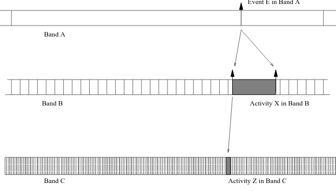
Band B

Band C Band A

Event E in Band A

Activity X in Band B

Activity Z in Band C

Events that are instantaneous in band A maymapto activities that have duration at some lower bandBwith a finer granularity. A key property of a band is theprecision it defines for its time scale. This requires the activity associated with event E (in band A) to have a maximum duration ofρ(the precision of band A - as measured in band B). An illustration of a three band system with the mapping of events to activities is shown in Figure 1. As noted earlier, the start and end of an activity are themselves represented as events.

The link between any two bands is expressed in terms of each band’s granularity and precision. Usually the finer of the two bands can be used to express these two measures for the broader band. Where physical time units are used for both bands these relations are straightforward. For example a band with a granularity of an hour and a precision of two minutes is easily linked to a band with a granularity of ten seconds and precision of half a second. The granularity relation is a link from one time unit (1 hour) in the higher band to 360 units in the lower band. The precision of one minute means that a time reference at the higher band (e.g., 3 o’clock) will map down to the lower band to imply a time reference (interval) between 2.59 and 3.01. In general, two bands are said to beorderedif the precision of one band is larger then the granularity of the other.

If an event,e, maps to an activity, a, then that activity has a unique signature event,sign(a), which corresponds toein the lower band. Behaviours are extended with activities. The mapping preserves the precedence relation between two higher band eventse1ande2by requiring that the signature events of their corresponding activitiesa1anda1in the lower band are similarly related, ie.sign(a1)¹sign(a2).

BehaviourMapping BehaviourActivities

à :E ↔ A sign:A 7→ E

dom(sign)⊆act

∀e:ev; a:act•eÃa⇒

e∈ev∧a∈act∧(band(a)⊏band(e)∧a∈dom(sign))

∀e:ev; a1,a2 :act•

band(a1) =band(a2)∧eÃa1∧eÃa2⇒a1 =a2

∀a:act•a∈dom(sign)⇒sign(a)∈events of(a)

∀e1,e2 :ev; a1,a2 :act•

e1Ãa1∧e2Ãa2∧band(a1) =band(a2)⇒

(e1¹e2⇒sign(a1)¹sign(a2))

3.9 Durations

which is represented by a natural number.

Interval=={I:P

1N|(∀t1,t2 :I; t:N•t1<t<t2⇒t∈I)}

An activity that has not terminated (ie. is not in the domain of “↓”) cannot be given a duration. The duration of a terminating activity is determined from its start and end events.

BehaviourDurations BehaviourMapping

duration: (E × E) 7→Interval act duration:A 7→Interval

dom(duration) ={e,f :ev|e¹f} ∀e,f,g,h:ev•e¹f ¹g¹h⇒

(∀I₁,I₂:Interval•duration(e,h) =I₁∧duration(f,g) =I₂⇒ I₂⊆I₁)

dom(act duration) =dom(↓)

∀a:dom(act duration)•act duration(a) =duration(↑a,↓a)

Any event in the upper band is mapped to an activity in the lower band whose duration is within the precision of the upper band (with respect to the lower band).

Precision is not only important in defining the bounds on what it means for an event to be instantaneous (in a band), it is also used to constrain what is meant by two events to be simultaneous in some band. Ifeandf are simultaneous in bandb (with precisionρwith respect to the lower bandc) then the signature events of the mapped activities must occur withinρin bandc. Similarly, two events can be defined to be ‘not simultaneous’ and may require some component of the system to test that this erroneous situation does not occur. Again, by placing such a requirement in the right band, the necessary tolerance on the implementation of the monitoring task is precisely defined.

BehaviourPrecision BehaviourDurations

∀e:ev; a:act•

eÃa⇒max(act duration(a))≤Precision(band(e),band(a))

∀e1,e2 :ev; a1,a2 :act•e1≃e2∧

e1Ãa1∧e2Ãa2∧band(a1) =band(a2)⇒

max(duration(sign(a1),sign(a2)))≤Precision(band(e1),band(a1))

3.10 Clocks

as external sources of time and temporal triggers abound [34]. So measures such as second, minute, hour, day, week, month, year, decade and century are now universal. But other time scales such as ‘generation’, ‘era’ and ‘age’ are also used in specific domains. In a different context the granularity of a band may relate to a physical property of the system, such as the rotation of the crank shaft for an engine control unit.

A frame of reference defines an abstract clock that counts ticks of the band’s granularity and can be used to give a time stamp to events and activities. A band may have more than one such abstract clock but they progress at the same rate. For example the day band will have a different abstract clock in each distinct geographical time zone.

We develop a consistent model of time by representing certain moments in the dynamics of a band as “clock tick” events, which are modeled just like any other event. When necessary, an event can be situated in absolute time (within the context of a defined band and clock) by stating a precedence relationship between the event and one or more clock ticks. So an event occurred between 2.00 and 3.00 (in the hour band) if the event occurred after the start of hour from 2.00 to 3.00 but before the end of that hour. Note this is different to saying the event occurred ‘at 2.00’. Here the implication is that it is simultaneous with the 2.00 event. So ‘I will arrive at 2.00’ is satisfied by arriving sufficiently close to the 2.00 event (within the precision of the hour band). However ‘I’ll will arrive by 3.00’ is quite different and allows the arrival event to occur anytime up to the 3.00 event.

A clock can be modeled as a sequence of clock-tick events of a given class, and hence a given time band. Successive clock-tick events are separated by one time unit in the granularity of the band. They are therefore never simultaneous.

4 State

In modelling state within the timeband framework there are a number of issues we need to take into account:

observations: within a particular time band, only a subset of the state variables (ob-servations) will be relevant,

nondeterminism: at the time interval corresponding to an event within a band, there may be a set of possible values of a state variable,

change-of-state events: for discrete state observations, changes in value correspond to change-of-state events,

accuracy: for a continuous state observation, there will be a maximum change over a time interval corresponding to the precision of the band, and

rate-of-change: for continuous observations, there will be a maximum rate of change over an interval of size the granularity of the time band.

– at a high time band one can view the door as eitheropenorclosed, with “instan-taneous” events to open or close it;

– at a lower time band the open and close events take time, and there are new activitiesopeningandclosing

– at a lower level still one may model how far open the door is by a percentage between 0% open (i.e., closed) and 100% open; this numeric measurement may either be discrete, with some granularity, or continuous; if it is discrete then, at a still lower time band, it may be discrete with a finer granularity.

This can be modeled by having different observation variables at different time bands.

4.1 States

The state space can be represented by a mapping from variable names, taken from the setV, to values, taken from the setX.

State[V,X] ==V 7→X

The above definition ofStateis generic in the sets of variables and values, for exam-ple, the instantiationState[{x,y},{0,1}]represents states with variable names from the set{x,y}and values from the set{0,1}. A state,σ∈V 7→X, maps each variable name in its domain to its value in that state. For simplicity we use the universal setX for all values, rather than each variable having values of a particular type. The set of observation variables in a particular time band is fixed, and hence it is useful to refer to sets of states, all of which have the same variables (i.e., domain).

StateSet[V,X] =={ss:PState[V,X]|(∀σ1, σ2:ss•dom(σ1) =dom(σ2))}

For example, ifxandyare variables and integers are values thensis a state andssis a state set.

s={x7→0,y7→1}

ss={{x7→0,y7→0},{x7→1,y7→0},{x7→1,y7→1}}

The “sets of states” view is adequate for a single sequential process controlling all the variables in the state, but if there are concurrent processes or an externally evolving environment, observation of the state at a particular time precision may observe one variable at one instant and another at a slightly different instant. Hence, if we don’t determine the order of observation of the variables, there is a set of values that we can observe for each variable at that time “instant”. This leads to a less determined representation of the states, in which each variable is mapped to a set of possible values.

4.2 Values views of the state

the set of states view doesn’t reflect the reality of observing multiple variables, all of which are evolving over time. For example, if we have two variablesxandywhich are both initially zero, and if in quick successionxchanges to one and thenychanges to one, then there is no point at which the state hasxwith value zero andywith value one. The set of states for this transition isss, above. However, a program sampling the two variables may first samplexand get zero and then sampleyand get one, ie. obtain a state{x7→0,y7→1}, which is not inss.

To address this issue we introduce a less determined representation of a set of states, which for each variable records the nonempty6set of values it has accumulated over all the states. This has less information than the equivalent set of states.

VState[V,X] ==V 7→P 1X

Note that a sets of values view, orvalues viewfor short, is a form of state with values replaced by sets of values:

VState[V,X] =State[V,P 1X]

As with states, we define the sets of values views, all of which have the same vari-ables.

VStateSet[V,X] ==StateSet[V,P 1X]

4.3 Relating a set of states to a values view

The set of statesssabove corresponds to the values viewsv.

sv={x7→ {0,1},y7→ {0,1}}

We define a functionvalues to represent this relationship so thatvalues(ss) = sv, where the notation{σ:ss•σ(v)}stands for the set of all values ofσ(v)forσinss.7

[V,X]

values:StateSet[V,X]→VState[V,X]

∀ss:StateSet[V,X]•

letvars=={v:V|(∃σ:ss•v∈dom(σ))} • values(ss) = (λv:vars• {σ:ss•σ(v)})

In the opposite direction, the set of states that may beapparentin a values view of the state can be extracted by considering all possible states such that each vari-able maps to an element of its set of possible values. For the values view sv, the corresponding set of apparent states is

apparent(sv) ={{x7→0,y7→0},{x7→1,y7→1}, {x7→0,y7→1},{x7→1,y7→0}}.

6 _HenceP

1rather thanP.

7 _{This is more commonly written{σ(v)|σ ∈ ss}but Z notation makes the fact thatσis a bound}

The functionapparentis defined as follows.

[V,X]

apparent:VState[V,X]→StateSet[V,X]

∀sv:VState[V,X]•

apparent(sv) ={σ:dom(sv)→X|(∀v:dom(sv)•σ(v)∈sv(v))}

We have two properties that relateapparentandvalues.

Theorem 1 For all values views, sv,

sv=values(apparent(sv)) (1)

and for all sets of states, ss,

ss⊆apparent(values(ss)) (2)

For example,

ss={{x7→0,y7→0},{x7→1,y7→0},{x7→1,y7→1}} sv=values(ss)

={x7→ {0,1},y7→ {0,1}}

apparent(sv) ={{x7→0,y7→0},{x7→1,y7→1}, {x7→0,y7→1},{x7→1,y7→0}} ⊃ss

values(apparent(sv)) ={x7→ {0,1},y7→ {0,1}}

=sv

Hence a set of states has potentially finer information than the corresponding values view.

4.4 Behaviour with state

Each time band has associated with it a set of variables that are observable in that band. Within a behaviour,ev val(e), returns the values view (over the observables of its band) that coincides with evente. For a discrete state variable, there is often a unique value, but if the event occurs close in time to a change of state then multiple values are possible to reflect our lack of knowledge of the actual value. For example, if an event is simultaneous with an hour band clockclkstriking 12 thenev valwill return{clk7→ {11,12}}. If the value of a continuous state variable is changing at the time of the event, then there is a range of values of the variable.

BehaviourState BehaviourPrecision observables:B →PV ev val:E 7→VState[V,X]

interval val:E × E 7→VStateSet[V,X]

dom(ev val) =ev

dom(interval val) ={e1,e2 :ev|band(e1) =band(e2)} ∀e:ev•dom(ev val(e)) =observables(band(e))

∀e1,e2 :ev•(e1,e2)∈dom(interval val)⇒

(∀σ:interval val(e1,e2)•dom(σ) =observables(band(e1)))

∀e1,e2,e3 :ev•e1≺e2≺e3⇒ev val(e2)∈interval val(e1,e3)

∀e1,e2 :ev•e1¹e2⇒interval val(e2,e1) ={} ∀e1,e2,e3,e4 :ev•e1¹e2¹e3¹e4⇒

interval val(e2,e3)⊆interval val(e1,e4)

∀e1,e2 :ev•e1≺e2⇒

(∀e:{e1,e2} •

(∃σ:interval val(e1,e2)•

(∀v:dom(σ)•ev val(e)(v)∩σ(v)6={})))

The values view associated with any event occurring within an interval must be in the values views of the interval. If two eventse2ande3are surrounded by eventse1and e4, the values views of the interval betweene2ande3must be contained in those of the interval betweene1ande4. For a nonempty interval the states corresponding to the end-point events “overlap” in values with some state within the interval.

The set of values views over an activity,a, is given byact val(a), which includes all the states between the start and end events of the activity, including at the start and end events.

BehaviourStateActivities BehaviourState

act val:A 7→VStateSet[V,X]

dom(act val) =act ∀a:act•

(∀σ:act val(a)•dom(σ) =observables(band(a)))∧

(∀e1,e2 :events of(a)• ev val(e1)∈act val(a)∧ interval val(e1,e2)⊆act val(a))

4.5 Change of state events

For discrete state, changes in value can be modeled by events. We can represent a change of state event in which variablevtakes on the new valuex, by the syntax

BehaviourStateChange BehaviourStateActivities

∀e₁:ev; v:V; x:X•e₁.class= (v:=x)⇒ x∈ev val(e₁)(v)∧

(∀e₂:ev•e₁≺e₂∧

¬(∃e:ev; y:X•e₁≺e≺e₂∧e.class= (v:=y))⇒

(∀σ:interval val(e₁,e₂)•σ(v) ={x}))

4.6 Mapping states

If an eventeis mapped to an activityain a lower band, then the values view at the event in the higher band corresponds to the union of the state values for the activity in the lower band.

BehaviourStateMapping BehaviourStateChange

∀e:ev; a:act•eÃa⇒

(∀v:observables(band(e))∩observables(band(a))• ev val(e)(v) ={x:X|(∃sv:act val(a)•x∈sv(v))})

4.7 Accuracy and rates of change

As discussed above, within a single band a numeric-valued variable may have an accuracy and a maximum rate of change. Its accuracy is the maximum amount it can change over a period of size the precision of the band, and its maximum rate of change is the maximum amount it can change over a period of size the granularity of the band.

Within a particular time band, the rate of change of a state variable can be viewed as the change in its value over a time unit within the band. We’ll illustrate this by discussing the maximum rate of change of a state variable,v.

– Within a given time band the maximum rate of change ofvmay ber, i.e.,vcan change by at mostrover one time unit in that band.

BehaviourRates BehaviourStateMapping accuracy:B →(V 7→R₎

rate:B →(V 7→R₎

∀b:B •letvars==dom(accuracy(b))•

vars=dom(rate(b))∧vars⊆observables(b)∧

(∀e:ev; v:vars•band(e) =b⇒

(∀x,y:ev val(e)(v)•abs(x−y)≤accuracy(b)(v)))∧

(∀e1,e2 :ev; v:vars•e1≺e2∧band(e1) =b∧band(e2) =b⇒

(∀σ₁, σ₂:interval val(e1,e2)•(∀x:σ₁(v); y:σ₂(v)• abs(x−y)≤rate(b)(v)∗max(duration(e1,e2)))))

∀e:ev; a:act•eÃa⇒

(∀v:dom(accuracy(band(e)))∩dom(rate(band(a)))•

rate(band(a))(v)∗max(act duration(a))≤accuracy(band(e))(v))

Satisfying the consistency condition has a special case if we consider the state vari-able to be uniform between two levels, oruniformfor short. If the granularity of the upper time band with respect to the lower time band isn, then for a uniform state variable the maximum rate of change in the lower time band will be at mostr/n. At a still lower time band with granularitymwith respect to the above lower band (and hence granularitym∗nwith respect to the upper time band) the maximum rate of change in this still lower time band will be at mostr/(m∗n). With a uniform state variable, as the size of the time unit of the band approaches zero the rate of change approaches the derivative of the state variable with respect to time.

5 Summary

Rather than have a single notion of time, the proposed framework allows a number of distinct time bands to be used in the specification or description of a system. System behaviours are always relative to (defined within) a band.

The above discussion has defined the timeband framework and introduced a num-ber of key notions that are central to the framework. Here we summarize these ideas:

– band– a subset of system behaviours (discrete and continuous) with similar tem-poral properties;

– system– a partially ordered set of bands;

– separation– the property of being able to assume that activities in lower (quicker) bands are instantaneous and the state of higher (slower) bands is unchanging; – granularity– the unit of time defined by a band;

– precision– the constraint on instantaneous behaviour within a band; – event– an instantaneous action within a band;

– activity– an action with duration within a band; – duration– a time interval between events;

– precedence– one event happening after another event; – simultaneous– two events occurring at the same instant;

– immediate– a precedence relation between two simultaneous events;

– mapping– a link between an event in one band to an activity in a lower band; – state– the observations available within a time band;

– set of values view– the observations over the period of an event; – change-of-state events– for discrete observations;

– accuracy– maximum “instantaneous” change in a continuous variable;

– rate-of-change– maximum rate of change of a continuous variable over a unit of time.

6 Towards a Language for Timebands

Having presented a model for the timeband framework it is then necessary to define a language that can be used to specify system requirements and behaviour. Such a language is derived from the abstract model. In this paper we do not attempt to provide a single, or even a complete, timeband language. Rather we illustrate features that such a language could usefully contain. These are used in a short example of the use of time bands in the Section 7.

6.1 Predicates

We represent a predicate over a state space,Σ, via the subset of states inΣthat satisfy the predicate.

Definition 1 (Predicate)For a state spaceΣ, a predicate is represented by a set of states.

Pred[Σ] ==P_Σ

We use the conventional notations, “∧”, “∨”, and “¬” instead of intersection, union, and complement of sets (with respect to the state spaceΣ), respectively, when deal-ing with predicates. As usual, the unary operators have higher precedence than the binary operators. Point-wise implication, denotedp⇒q, is defined as¬p ∨q, and point-wise equivalence is denoted byp⇔q. Universal implication, denotedp⇛q, is defined as (∀σ • σ ∈ p ⇒ σ ∈ q), or more succinctly as p ⊆ q. Universal equivalence is denotedp≡q.

6.2 Predicates on sets of states

Definition 2 (All states and some states)

[Σ]

¤_{* :}Pred[Σ]→Pred[P 1Σ]

⊡:Pred[Σ]→Pred[P 1Σ]

∀p:Pred[Σ]; ss:P 1Σ•

(ss∈(¤_*p)⇔(∀σ:ss•σ∈p))∧

(ss∈(⊡p)⇔(∃σ:ss•σ∈p))

We promote the boolean operators to predicates on sets of states in the obvious way (because they are defined as predicates, but over sets of states rather than states). We have the following properties of “all states” and “some state” when combined with logical operators.

¬ ¤_*p ≡ ⊡(¬p) (3)

¤_*p⇛ ⊡p (4)

¤_*p∧¤_*q ≡ ¤_{* (}p∧q) (5) ⊡p∨⊡q ≡ ⊡(p∨q) (6) ¤_*p∨¤_*q⇛ ¤_{* (}p∨q) (7) ⊡(p∧q)⇛ ⊡p∧⊡q (8)

Note that property (4) is valid because the sets of states must be non-empty.

Theorem 2 Given state predicates p and q,

(⊡p⇒¤_*q)⇛(¤_{* (}p⇒q)) (9)

Proof.

⊡p⇒¤_* q

≡by the definition of implication ¬ ⊡p∨¤_*q

≡by (3) ¤_*¬p∨¤_*q ⇛by (7)

¤_{* (}¬p∨q)

≡by the definition of implication ¤_{* (}p⇒q)

6.3 Predicates on values views

We refer to a predicate on a values view of the state as avalues predicate.

Definition 3 (Values predicate)

VPred[V,X] ==Pred[VState[V,X]]

We promote a predicate,p, on a single state, to a predicate on a values view in two ways. Ifp holds for all apparent states (see Section 4.3) derivable from the values view,sv, we sayp definitelyholds forsv, writtensv∈⊛p, and ifpholds for at least one apparent state derivable fromsv, we sayp possiblyholds forsv, writtensv∈ ⊙p.

Definition 4 (Definitely and possibly)

[V,X]

⊛_:Pred[State[V,X]]→VPred[V,X]

⊙:Pred[State[V,X]]→VPred[V,X]

∀p:Pred[State[V,X]]; sv:VState[V,X]•

(sv∈(⊛p)⇔(∀σ:apparent(sv)•σ∈p))∧

(sv∈(⊙p)⇔(∃σ:apparent(sv)•σ∈p))

We promote the boolean operators to values predicates in the obvious way because values predicates are predicates, but over values views rather than states.

In the example considered in Section 7, if the methane in a coal mine shaft is ever over a critical level, then to avoid causing an explosion, the pump extracting water from the mine must be off. We can formalise this property by the following values predicate.

⊙(methane≥Critical)⇒⊛(pump=Off)

If the methane is possibly critical at some instant (i.e., the values view includes an apparent state in which the methane is critical), then the pump is definitely off (i.e., it is off for all apparent states).

From Definitions 2 and 4, the “definitely” and “possibly” operators are related to “all states” and “some state” as follows for all values views,sv.

sv∈⊛p⇔apparent(sv)∈¤_*p (10) sv∈ ⊙p⇔apparent(sv)∈⊡p (11)

Hence, we have the following properties directly derivable from the properties of predicates on sets of states (3)–(8).

¬ ⊛p ≡ ⊙(¬p) (12)

⊛p⇛⊙p (13)

There are two interesting properties of definitely (⊛) and possibly (⊙) that don’t hold for “all states” (¤_*) and “some states” (⊡).

Theorem 3 If the free variables occurring in the predicates p and q are disjoint, then

⊙p∧ ⊙q≡ ⊙(p∧q) (18) ⊛(p∨q)≡⊛p∨⊛q (19)

If the set of free variables occurring in the predicatepisw, andσ1 andσ2are two

states that agree on all the variables inw, (i.e.,w⊳σ1=w⊳σ2, wherew⊳σis the

stateσrestricted to just those variables in the setw), thenσ1∈p⇔σ2∈p.

Proof. We focus on property (18) because (19) can be derived from it using⊛p =

¬ ⊙ ¬ p. The reverse implication is property (17) above. In the forward direction, if we assumesv∈ ⊙pandsv ∈ ⊙q, then(∃σ:apparent(sv)• σ∈ p)and(∃σ:

apparent(sv)•σ∈q). Hence letσ1∈p∩apparent(sv), andσ2∈q∩apparent(sv).

Ifwis the set of free variables occurring inp, we letσ= (w⊳_σ1)∪(w−⊳_σ2), where w⊳σis the stateσrestricted to just the variables inwandw−⊳σisσrestricted to the variables not inw. Becausepdepends only on variables inwandw⊳σ=w⊳σ₁, it follows thatσ ∈p. Similarly, becauseqonly depends on variables not inw,σ∈q. Finally, because bothσ₁andσ₂are inapparent(sv),σ∈apparent(sv). Hence(∃σ:

apparent(sv)•σ∈p∧q), i.e.,sv∈ ⊙(p∧q). 2

Note that (18) holds for⊙but not⊡. For example, if

ss={{x7→0,y7→0},{x7→1,y7→0},{x7→1,y7→1}}

we havess∈⊡(x= 0)∧⊡(y= 1)but notss∈⊡(x= 0∧y= 1). Using Theorem 3 we can show the following theorem.

Theorem 4 Provided the free variables of p and q are disjoint,

⊛(p⇒q)≡(⊙p⇒⊛q)

Proof.

⊛(p⇒q)

≡⊛(¬p∨q)

≡Theorem 3; free variables in the two disjuncts are disjoint ⊛(¬p)∨⊛q

≡ ¬ ⊙p∨⊛q ≡ ⊙p⇒⊛q

6.4 On the relationship between reality and observation

For each event there is an interval over which the event occurs and a set of actual states,ss, over that interval. The corresponding values view isvalues(ss). From prop-erty (2), i.e.,ss⊆apparent(values(ss)), if we want to show a property,p, holds for all actual states inss, it is sufficient to show the stronger property thatpholds for all states inapparent(values(ss)), i.e.,⊛pholds forvalues(ss). Similarly, if we know a propertypholds for some actual state inss, we can deduce⊙pforvalues(ss). These relationships are captured by the following theorem.

Theorem 5 For any set of actual states, ss,

values(ss)∈⊛p⇒ss∈¤_* p (20) ss∈⊡p⇒values(ss)∈ ⊙p (21)

Consider the simple case in which we are only dealing with one free variable,x, in a predicate, e.g., the predicate is of the form⊛₍x∈ S)or ⊙(x ∈ S), whereSis constant over the observation interval, then⊛(x∈S)in the values view is equivalent to¤_{* (}x∈ S)in reality, and⊙(x ∈ S)in the values view is equivalent to⊡(x ∈ S)

in reality. Special cases of these predicates are comparisons of a variable with an expression,C, that is constant over the observation interval, e.g.,x=Corx<C.

If one samples a variable, x, in the environment, and gets the valueC, one can deduce⊡(x=C), which is equivalent to⊙(x=C). Similarly, by samplingywe may deduce⊡(y =D), which is equivalent to⊙(y =D). By Theorem 3 these samples allow one to deduce ⊙(x = C ∧ y = D)but not the stronger condition ⊡(x =

C ∧y=D). This formalises the property that sampling two boolean variables,top andbottom, introduced in Section 2. Getting two sample values, e.g.,trueandtrue, does not allow one to deduce that the two variables simultaneously have those values (i.e., we can’t deduce⊡(top ∧ bottom)), but we can deduce the weaker property ⊙(top∧bottom). That is

ss∈⊡(top∧bottom)⇒values(ss)∈ ⊙(top∧bottom)

but not the other way around, in general. Note that⊙(top ∧ bottom) ≡ ⊙top ∧ ⊙bottom, but we only have⊡(top∧bottom)⇛ ⊡top∧⊡bottom, in general.

6.5 Application to state model

In this section we develop some notation for using values predicates with the values view model. Given a behaviour and an evente,ev val(e)gives the values view corre-sponding to evente. For a values predicate,p, we introduce the notationp@eto state thatpholds for the values view corresponding toe, i.e.,

p@e⇔ev val(e)∈p