Scheduling divisible loads to optimize the computation time and cost

This is a repository copy of Scheduling divisible loads to optimize the computation time

and cost.

White Rose Research Online URL for this paper:

http://eprints.whiterose.ac.uk/79244/

Proceedings Paper:

Shakhlevich, NV (2013) Scheduling divisible loads to optimize the computation time and

cost. In: Altmann, J, Vanmechelen, K and Rana, OF, (eds.) Economics of Grids, Clouds,

Systems, and Services, 10th International Conference (GECON 2013), Proceedings. 10th

International Conference (GECON 2013), 18-20 Sep 2013, Zaragoza, Spain. Springer ,

138 - 148. ISBN 978-3-319-02413-4

https://doi.org/10.1007/978-3-319-02414-1_10

Reuse

Unless indicated otherwise, fulltext items are protected by copyright with all rights reserved. The copyright exception in section 29 of the Copyright, Designs and Patents Act 1988 allows the making of a single copy solely for the purpose of non-commercial research or private study within the limits of fair dealing. The publisher or other rights-holder may allow further reproduction and re-use of this version - refer to the White Rose Research Online record for this item. Where records identify the publisher as the copyright holder, users can verify any specific terms of use on the publisher’s website.

Takedown

If you consider content in White Rose Research Online to be in breach of UK law, please notify us by

Scheduling Divisible Loads to Optimize the Computation Time

and Cost

Natalia V. Shakhlevich

School of Computing, University of Leeds, Leeds LS2 9JT, U.K.

Abstract

Efficient load distribution plays an important role in grid and cloud applications. In a typical problem, a divisible load should be split into parts and allocated to several processors, with one processor responsible for the data transfer. Since processors have different speed and cost characteristics, selecting the processors order for the transmis-sion and defining the chunk sizes affect the computation time and cost. We perform a systematic analysis of the model analysing the properties of Pareto optimal solutions. We demonstrate that the earlier research has a number of limitations. In particular, it is generally assumed that the load should be distributed so that all processors have equal completion times, while in fact there often exists a dominating schedule with non-simultaneous finishing times of the processors. Moreover, fixing the processor sequence in the non-decreasing order of the cost-characteristic may be appropriate only for Pareto-optimal solutions with relatively large deadlines; Pareto-optimal schedules for tight deadlines may have a different order of processors. We conclude with an efficient algorithm for finding the time-cost tradeoff.

Keywords: scheduling, divisible load, time/cost optimization

1

Introduction

Parallel computer systems have given rise to new scheduling models that go beyond the classical scheduling theory. While in a traditional scheduling model a task can be processed by one machine at a time, a new feature of multiprocessor computations is the ability to split tasks into several parts and to process them simultaneously by different processors, see, e.g., [5, 8]. An additional feature of modern Grid computing and cloud computing systems is the introduction of the cost factor, see, e.g. [2, 6, 10]. This study is motivated by the lack of theoretical research in the area and some inaccuracies which can be found in the earlier research.

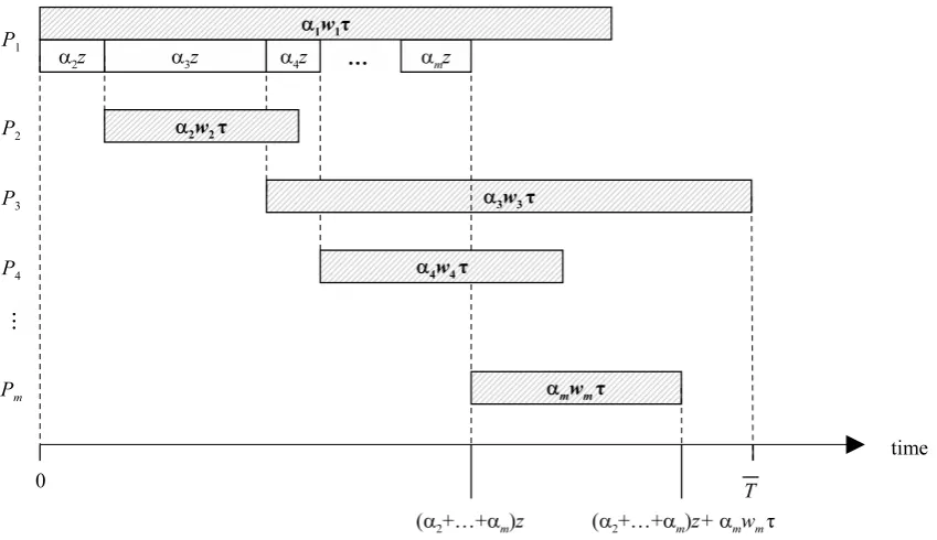
We consider the network model described in [7]. There is a set P = {P1, P2, . . . , Pm}

of m processors connected via a bus type communication medium. One processor of the set P is selected as a master processor to receive a divisible load of size τ and to divide it into portions of size α1τ, α2τ,. . . , αmτ, ∑mk=1αk = 1, which are then transmitted to slave

processors from P to perform required computations.

The processors have different computation speeds and for each processor Pk ∈ P the

inverse of the speedwkis given. This implies that the load of sizeαkτ allocated to processor

Pk requires computation timeαkwkτ.

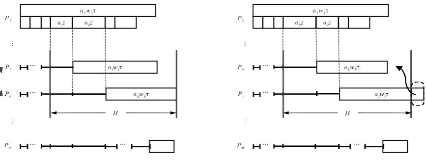
IfP1 is selected as a master processor and the transmission sequence isP2,P3,. . ., Pm,

then P1 can start processing its own load of size α1τ at time 0 and at the same time it can start transmitting the relevant portions of the load first to P2, then toP3, etc., until the last

portion is transmitted to Pm, see Fig. 1. Ifz is the time needed to transmit the whole load

of size τ, then the communication time for transmitting the portion αkτ to processor Pk is

αkz.

Figure 1: An example of a schedule with master processor P1 and transmission sequence P2, . . . , Pm

With the selected transmission order, processorP1 completes its portion of computation at time

T1 =α1w1τ. (1)

Processor Pk, 2≤k≤m, receives its portion of the load at time∑ki=2αiz and immediately

after that it can start computation, which takes αkwkτ time. Thus processor Pk completes

its portion of the load at time

Tk = k

∑

i₌₂

αiz+αkwkτ.

The finish time T of the load is defined as the makespan of the schedule; it is equal to the maximum completion time among all processors,

T = max

1≤k≤m{Tk}. (2)

after “αmz”, and formula (1) should be replaced by

T1 =

m

∑

i₌₂

αiz+α1w1τ. (3)

Processing the load in accordance with the load distributionα1,α2,. . . , αm incurs

com-putation cost which depends on processors’ costs. Following the notation from [7], we denote the cost of using processor Pk∈ P during one time unit byck so that the cost of performing

the portion of the load αkwkτ by processor Pk is ckαkwkτ. The overall cost of using all

processors P is therefore

K=

m

∑

k₌₁

ckαkwkτ.

Thus a scheduleS is given by

- the transmission sequence with the first processor of the sequence selected as a master processor

and

- the load distribution α1,α2,. . . ,αm with∑mk=1αk = 1.

In this paper we assume that the processors are numbered so that

c1w1≤c2w2 ≤ · · · ≤cmwm. (4)

The quality of a scheduled is measured in terms of the two characteristics: maximum completion time T and computation costK. As a solution of a bicriteria problem we accept the set of Pareto optimal points defined by the break-points of the so-calledefficiency frontier. In a pair of the associated single criterion problems,

min K

s.t. T ≤T (5)

and

min T s.t. K≤K

one of the objectives is bounded while the other one is to be minimized. Here T and K are threshold values of the load finish time and computation cost, respectively.

2

Finding the Efficiency Frontier

In the (T, K)-space, the set of Pareto-optimal points represents a time-cost efficiency frontier. We start with an overview of the main outcomes of [7] and then proceed with the description of additional steps needed to find a correct efficiency frontier.

It is claimed in [7] that all break-points correspond to the schedules of a special type: the processor sequence is the same for all break-points and it is (P1, P2, . . . , Pm); only a subset

of the several first processors have a non-zero load, while the remaining processors are idle. Recall that processors are numbered in accordance with (4).

To represent the described schedules formally, introduce notation (P∗

1, P2∗, . . . , Pk∗, −,

. . . ,−) to indicate that processorsP1, P2, . . . , Pk are fully loaded completing computation at

time T, while the remaining processors Pk₊₁, Pk₊₂, . . . , Pm are idle. Then the set of the

break-points established in [7] is of the form:

( P∗

1, −, −, · · ·, −, −, · · ·, −, − ) ( P₁∗, P₂∗, −, · · ·, −, −, · · ·, −, − ) ( P∗

1, P2∗, P3∗, · · ·, −, −, · · ·, −, − ) . ..

( P∗

1, P2∗, P3∗, · · ·, Pk∗, −, · · ·, −, − )

( P∗

1, P2∗, P3∗, · · ·, Pk∗, Pk∗₊₁, −, − )

. .. ( P∗

1, P2∗, P3∗, · · ·, Pk∗, Pk∗₊₁, · · ·, Pm∗−1, − ) ( P₁∗, P₂∗, P₃∗, · · ·, Pk∗, P

∗

k+1, · · ·, Pm∗−1, Pm∗ )

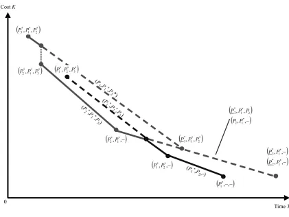
The graphical representation of the efficiency frontier from [7] for the case ofm= 3 pro-cessors is shown in Fig. 2. The three break-points, considered right to left, are (P∗

1,−,−), (P∗

1, P2∗,−) and (P1∗, P2∗, P3∗). When transition from (P1∗,−,−) to (P1∗, P2∗,−) is performed, the load from P1 is re-distributed to P2 until both processors have equal completion time; the intermediate points belonging to that segment of the efficiency frontier are denoted by (P∗

1, P2,−), where notation P2 in the schedule description indicates that processor P2 is partly loaded. Similarly, when transition from (P₁∗, P₂∗,−) to (P₁∗, P₂∗, P₃∗) is performed, the load from P1 and P2 is re-distributed to P3 until all three processors have equal comple-tion time; the intermediate points belonging to that segment are denoted by (P∗

1, P2∗, P3), where notation P3 indicates that processor P3 is partly loaded, while notation P1∗, P2∗ im-plies that the corresponding processors are fully loaded completing their portions of the load simultaneously.

It appears that the efficiency frontier is more complicated than the one presented in [7]. In particular, it includes also the points with the processor order different from (P1, P2, . . . , Pm).

In fact, the efficiency frontier can be found as the set of non-dominating segments of m curves Cℓ, ℓ = 1, . . . , m. Each curve Cℓ consists of linear segments and corresponds to

a processor sequence with a fixed master processor Pℓ. As we prove in the appendix, in

the class of schedules with a fixed master processor Pℓ, an optimal processor sequence is

(Pℓ, P₁, P₂, . . . , Pℓ₋₁, Pℓ₊₁, . . . , Pm). If ℓ >1, then the first ℓ−1 breakpoints (considered in

the (T, K)-space from right to left) correspond to schedules in which the master processor Pℓ performs only data transmission and does not perform ant computation; the next

break-point involves all ℓ processors fully loaded, so that the master processor Pℓ performs both,

data transmission and computation; in the remaining m−ℓ schedules,ℓfirst processors are fully loaded together with an increasing number of additional slave processors with indices larger than ℓ.

Formally, the break-points of the curve Cℓ with a fixed master processor Pℓ are of the

form:

processor Pℓ

does not perform any computation, only data transmission               

( Pℓ, P₁∗, −, −, · · ·, −, −, · · ·, −, − )

( Pℓ, P₁∗, P₂∗, −, · · ·, −, −, · · ·, −, − )

( Pℓ, P₁∗, P₂∗, P₃∗, · · ·, −, −, · · ·, −, − )

. .. −,

( Pℓ, P₁∗, P₂∗, P₃∗, · · ·, Pℓ∗₋₁, −, · · ·, −, − )

processor Pℓ

performs computation (until T) and data transmission

              

( P∗

ℓ, P1∗, P2∗, P3∗, · · ·, Pℓ∗₋₁, −, · · ·, −, − )

( Pℓ∗, P

∗

1, P2∗, P3∗, · · ·, Pℓ∗−1, Pℓ∗+1, · · ·, −, − ) . ..

( Pℓ∗, P

∗

1, P2∗, P3∗, · · ·, Pℓ∗−1, Pℓ∗+1, · · ·, Pm∗−1, − ) ( P∗

Figure 2: Efficiency frontier defined in [7] for the case ofm= 3 processors and the associated schedules (idle processors are omitted)

Here notation Pℓ, which appears in the first ℓ−1 schedules, indicates that processor Pℓ

performs only data transmission and no computation.

The intermediate points of the segments connecting the firstℓ−1 break-points correspond to the re-distribution of the load to one additional slave processor, without involving the master processorPℓin the computation; the previously loaded slave processors complete their

load simultaneously. The transition from the break-point(Pℓ, P₁∗, P₂∗, . . . , Pℓ∗−1,−, . . . ,−

) to

the ℓ-th break-point (P∗

ℓ, P1∗, P2∗, . . . , Pℓ∗₋₁,−, . . . ,−

)

corresponds to the reallocation of the load from the slave processors P₁∗, P₂∗, . . . , Pℓ∗−1 to the master processorPℓ, keeping the slave

processors completing their computation simultaneously. Finally, the intermediate points of the segments the last m−ℓ break-points correspond to the re-distribution of the load to one additional slave processor that follows the current busy processors in the processor sequence (Pℓ, P1, P2, . . . , Pℓ−1, Pℓ+1, . . . , Pm); all previously loaded processors complete their

load simultaneously.

Figure 3: Three curves

C1 coonecting (P1∗,−,−), (P1∗, P2∗,−), (P1∗, P2∗, P3∗)

C2 coonecting (P∗2, P1∗,−), (P2∗, P1∗,−), (P2∗, P1∗, P3∗)

C2 coonecting (P∗3, P1∗,−), (P3∗, P1∗, P2∗), (P3∗, P1∗, P2∗)

and the trade-off curve (in solid lines) consisting of non-dominating segments and their parts

to left:

(i) the right-most segment of the curve C1 that connects (P1∗,−,−) and (P1∗,P2∗,−);

(ii) a part of the second segment ofC1 that connects (P1∗, P2∗,−) and (P1∗, P2∗, P3∗) until its intersection point with the first segment of C2;

(iii) a part of the segment of the curve C2 connecting (P2, P1∗,−) and (P2∗, P1∗,−) starting at the right end with the previously defined intersection with C1;

(iv) the full segment of the curve C2 connecting (P2∗, P1∗,−) and (P2∗, P1∗, P3∗);

(v) a part of the last segment of the curve C3 connecting (P3, P1∗, P2∗) and (P3∗, P1∗, P2∗); its right-most T-value corresponds to the T-value of the left end (P₂∗, P₁∗, P₃∗) of the previous segment.

Notice that the resulting efficiency frontier is not convex and even not continuous. While it is possible to prove that some points of the curvesC1,C2, andCmalways dominate

each other (for example, (P∗

1,−,−, . . . ,−) always dominate (Pk, P₁∗,−, . . . ,−) for any 1 <

k≤m), the dominance relation between other points can vary depending on the specificci

-and wi-values. For example in the three processor case, the may be no intersection point

between curves C1 and C2, so that the whole curve C1 dominates all points of the curve C2. We demonstrate in the full version of the paper that for each curve Cℓ, all its

break-points can be found in O(m2) time since each subsequent break-point can be defined from the previous one in O(m) time by re-calculating the associatedαi-values, 1≤i≤m. Thus

all break-points of the curves C1,C2, . . . , Cm can be found inO(m3) time.

Having constructedm(m−1) segments of the curvesC1,C2, andCm, the required efficiency

frontier is found as the lower boundary among the curves.

3

Conclusions

In this paper, we have performed a systematic analysis of the problem of scheduling a divisible load on m processes in order to minimize the computation time and cost. An efficient algo-rithm for solving the bicriteria version of the problem defines optimal processor sequences for different segments of the efficiency frontier and the corresponding optimal load distribution among the processors.

Our study demonstrates that the earlier research [7] has a number of limitations. Some assumptions result in incorrect major conclusions. In particular, it is generally assumed in [7] that the load should be distributed so that all processors complete their portions simultane-ously, while as we show, there often exists a dominating schedule with non-simultaneous fin-ishing times of the processors. Moreover, fixing the processor sequence in the non-decreasing order of the cost/speed characteristic given by (4) may be appropriate only for Pareto-optimal solutions with relatively large deadlines; optimal schedules for tight deadlines may have a different order of processors with master processor Pℓ, 1 < ℓ ≤ m, moved in front of slave

processors P1, P2, . . . , Pℓ₋₁, Pℓ₊₁, . . . , Pm.

The described model with a single divisible load provides a foundation for more ad-vanced models which better describe various real-world scenarios. Further generalizations include multiple divisible loads, bandwith dependent formulae for calculation transmission times, multi-installment load distribution, multi-round schedules and more complex network

topologies. An attempt to generalize the results for the case of a more complex cost function that includes data transmission costs in addition to computation costs is presented in [3]. Clearly, a study of more complex models should rely on accurate analysis of the simplified model.

Appendix

The validity of the described algorithm follows from a number of properties of optimal schedules. The properties are proved for a single-criterion version of the problem (5) for a fixed makespan parameter T. Since T may take different values, the properties are correct for all schedules of the efficiency frontier.

The first two propositions provide a justification for fixing a processor sequence in an optimal solution; the third proposition establishes how the load should be distributed in an optimal solution.

We assume that processors are numbered in accordance with (4). Initially we consider an arbitrary processor sequence which can be different from the sequences listed in Section 2.

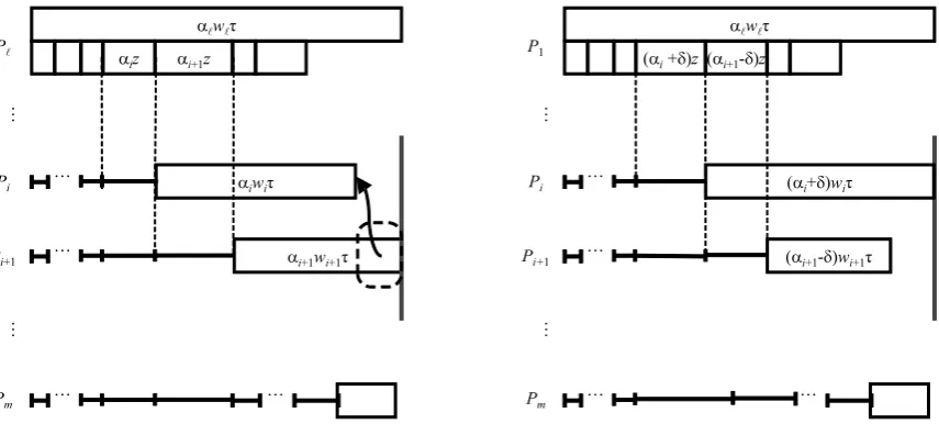
Proposition 1 ‘Swapping Two Neighbour Slave Processors’

Consider schedule S in which two neighbour slave processors Pi and Pk in the processor

sequence compute portions of load αi andαkand have finishing timesTi andTk, respectively.

It is always possible to change the order of Pi and Pk in the processor sequence so that in a

new schedule S′ the loads are α′i and αk′, processor finish times are T

′

i andTk′ and

(a) the loads are re-distributed so that α′

i =αi−δ andα′k=αk+δ for 0≤δ ≤αi;

(b) the load on other processors remains the same;

(c) the maximum finish time of processors Pi andPk does not increase:

max{T′

i, Tk′} ≤max{Ti, Tk}.

Proof. Introduce notation Θ for max{Ti, Tk}. We consider the two cases depending on

whether processor Pi finishes its portion of the load earlier thanPk or not.

Case 1: in the initial schedule S,Ti ≤Tk. This implies that

αiwiτ ≤αk(z+wkτ). (6)

In the initial scheduleS, we denote by H the length of the time interval from the start of αizuntil Θ =Tk,

H =αiz+αk(z+wkτ).

Consider schedule S′ _{obtained from S by swapping P}

k and Pi. If in S′ condition (c) is

satisfied, then Proposition 1 holds. Otherwise we have a schedule shown in the right-hand-side of the figure, with Ti′ >Θ (notice, that Tk′ cannot exceed Θ sinceαk(z+wkτ) < H).

In order to achieve condition (c), we need to move part δ ≤αi of the Pi-load toPk, so that

in the resulting schedule S′ _{the load onP}

i isα′i =αi−δ and the load on Pk is α′k=αk+δ.

The following inequalities should be satisfied:

α′

i ≥0, (load allocated toPi does not become negative),

α′

k(z+wkτ)≤H, (Tk′ does not exceed Θ),

α′kz+α

′

i(z+wiτ)≤H, (Ti′ does not exceed Θ).

Figure 4: Changing the sequence of Pi and Pk in Case 1

It follows that

αi−δ≥0, ⇒ δ ≤ai,

(αk+δ) (z+wkτ)≤αiz+αk(z+wkτ) ⇒ δ ≤ _z+α_wiz

kτ,

(αk+δ)z+ (αi−δ) (z+wiτ)≤αiz+αk(z+wkτ) ⇒ δ ≥αi− αkwk

wi .

The second and the third inequalities imply that

αi−

αkwk

wi

≤δ≤αi−

αiwkτ

z+wkτ

, (8)

while the first condition δ ≤ ai is redundant since _z+α_wiz

kτ ≤ai. Notice, that (8) is feasible

since

αkwk

wi

≥ αiwkτ

z+wkτ

by (6).

Case 2: in the initial scheduleS,Ti > Tk:

αiwiτ > αk(z+wkτ). (9)

In the initial schedule S, we denote by G the length of the time interval from the start of αizuntil Ti,

G=αi(z+wiτ).

After swapping Pk and Pi, if the load is kept unchanged, we obtain schedule S′ with

T′

i >Θ, while Tk′ ≤Θ. Hence we need to move part δ ≤αi of the Pi-load to Pk, so that in

the resulting scheduleS′ _{the load onP}

i isα′i =αi−δ and the load onPk isα′k=αk+δ. We

need to guarantee that inequalities (7) with H replaced by Gshould be satisfied. It follows that

αi−δ≥0, ⇒ δ≤ai,

(αk+δ) (z+wkτ)≤αi(z+wiτ) ⇒ δ≤

αi(z+wiτ)

z+wkτ −αk,

(αk+δ)z+ (αi−δ) (z+wiτ)≤αi(z+wiτ) ⇒ δ≥ αkz

wiτ.

Figure 5: Changing the sequence of Pi and Pk in Case 2

It remains to show that condition

αkz

wiτ

≤δ≤min {

αi,

αi(z+wiτ)

z+wkτ

−αk

}

is feasible. Indeed, if the smallest value in the right hand side is αi, then

αkz

wiτ

< ai

due to (9). Alternatively, if αi is the largest value in the r.h.s., then

r.h.s.−l.h.s.= αi(z+wiτ) z+wkτ

−αk−

αkz

wiτ

= αiwiτ−αk(z+wkτ) wiτ(z+wkτ)

(z+wiτ).

The numerator in the last expression is positive due to (9), so that a feasible δ that lies in-between the l.h.s and the r.h.s. does exist.

Proposition 2 ‘Non-decreasing Sequence of ciwi for Slave Processors’

If the master processor Pℓ is fixed, then an optimal processor sequence is (Pℓ, P1, P2, . . . , Pℓ₋₁, Pℓ₊₁, . . . , Pm).

Proof. Suppose in an optimal schedule there are two neighbour processors Pi and Pk, Pi

precedes Pk and ciwi > ckwk. Then such a schedule is not optimal. Indeed, changing the

order Pi and Pk in the processor sequence, as described in Property 1, leads to a schedule

S′ with the same finish time of the load and α′i = αi −δ, α′_k = αk+δ. Since the load of

other processors does not change, the computation cost changes from KtoK′_andK′_{−K =} (ckwk−ciwi)τ δ <0.

Given a schedule, letT be its makespan, see (2). Depending on processors’ finish times, we classify them as fully loaded, partly loaded or idle. ProcessorPi is busy ifTi≥0, and it

is idle otherwise. To be precise, we call processor Pi fully loaded if Ti = T and it ispartly

loaded if 0< Ti < T. Notice that the master processor can be idle if its performs only data

Proposition 3 ‘Unique Partly Loaded Processor’

Consider a class of schedules with master processor Pℓ and an optimal schedule with

pro-cessor sequence (Pℓ, P1, P2, . . . , Pℓ−1, Pℓ+1, . . . , Pm). Let k be the largest index among busy

processors, 1 ≤ k ≤ m. Then all processors with smaller indices P₁, P₂, . . . , Pk₋₁ are fully

loaded and all processors with larger indices Pk+1, Pk+2, . . . , Pm are idle.

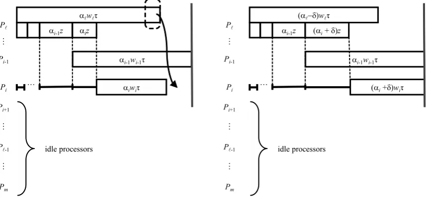
Proof. We first show that there cannot be an idle or partly loaded slave processor, after which there is another (partly or fully) loaded processor. Suppose in schedule S processor Pi is idle or it is partly loaded, whilePi+1 has a non-zero load. Then the load ofPi+1can be re-distributed by moving part δ of that load from Pi₊₁ to Pi, 0 < δ ≤αi₊₁, so that in the

resulting schedule S′,

α′i₊₁ = αi+1−δ, α′i = αi+δ,

see Fig. 6. As a result of this transformation, the finish time of Pi increases (due to the

increase in the transition timeα′

iz > αizand the increase in the computation time α′iwiτ >

αiwiτ) while the finish time ofPi₊₁ decreases (due to the decrease in the computation time

α′

i+1wi+1τ < αi+1wi+1τ; the total transition time does not change since (α′i+α′i+1

) z = ((αi+δ) + (αi₊₁−δ))z= (αi+αi₊₁)z). The finish times of the remaining processorsPi₊₁,

. . . , Pm does not change decrease. The largest feasible value ofδeither makesPi fully loaded

or makesPi+1 idle. Since ciwi≤ci+1wi+1 by (4), the cost of the resulting schedule does not increase.

Figure 6: Re-distributing the load between two slave processors

In what follows we consider an optimal schedule in which the last slave processor with non-zero load is Pk, all slave processors with smaller indices are fully loaded and all slave

processors with larger indices are idle. If index ℓ of the master processor Pℓ satisfiesℓ > k,

so that cℓwℓ ≥ckwk and that processor has a non-zero load, then we re-distribute the load

from Pℓ toPk. In the resulting schedule S′,

α′ℓ = αℓ−δ,

α′k = αk+δ,

where 0< δ≤αℓ. This transformation does not affect other processors with non-zero load,

but decreases the cost, see Fig. 7.

Figure 7: Re-distributing the load from Pℓ toPi,i < ℓ

If inS′_,P

ℓbecomes idle, Proposition 3 is proved. OtherwisePk becomes fully loaded and

we perform a similar transformation by moving the load from Pℓ toPk₊₁, . . . , Pℓ₋₁ untilPℓ

becomes idle or all slave processors with indices smaller than ℓbecome fully loaded.

Finally, consider that case that indexℓof the master processorPℓ satisfiesℓ < k, so that

cℓwℓ ≤ckwk. We re-distribute the load from Pk to Pℓ so that either Pk becomes idle or Pℓ

becomes fully loaded. As a result of this transformation, the finish time ofPkdecreases (due

to the decrease in the transition time α′

kz < αkz and the decrease in the computation time

α′

kwkτ < αkwkτ), and the finish time ofPℓ increases (due to the increase in the computation

time α′ℓwℓτ < αℓwℓτ). The largest feasible value of δ either makes Pℓ fully loaded or makes

Pk idle; the cost of the resulting schedule does not increase.

It follows from Propositions 1-3 that in a class of schedules with a fixed master processor Pℓ all optimal schedules have processor order (Pℓ, P₁, P₂, . . . , Pℓ₋₁, Pℓ₊₁, . . . , Pm) and for a

given makespan threshold valueT, an optimal schedule can be constructed by loading in full processors in the order P1, P2, . . . , Pk−1 until the remaining load can be processed by Pk.

Varying theT-values we conclude that all optimal schedules in that class belong to the curve

Cℓ defined in Section 2.

Acknowledgements

This research was supported by the EPSRC funded project EP/G054304/1 “Quality of Ser-vice Provision for Grid applications via Intelligent Scheduling”.

References

[2] Buyya, R., Abramson, D., Venugopal, S.: The grid economy, Proceedings of the IEEE 93 (2005) 698–714

[3] Charcranoon, S., Robertazzi, G.R., Luryu, S.: Parallel processor configuration design with processing/transmission costs, IEEE Trans. on Computers49 (2000) 987–991.

[4] Chuprat, S., Baruah, S.: Real-time divisible load theory: incorporating computation costs, Proceedings of the 17th IEEE International Conference on Embedded and Real-Time Computing Systems and Applications

[5] Drozdowski, M.: Scheduling for Parallel Processing, Springer, London, 2009

[6] Kumar, S. Dutta, K., Mookerjee, V.: Maximizing business value by optimal assignment of jobs to resources in grid computing, European J. of Oper. Res.194 (2009) 856–872

[7] Sohn, J., Robertazzi, T.G. and Luryi, S.: Optimizing computing costs using divisible load analysis, IEEE Trans. Parallel and Distributed Systems9 (1998) 225–234

[8] Robertazzi, T.G.: Ten reasons to use divisible load theory, IEEE Computer 36 (2003) 63–68

[9] van Hoesel, S., Wagelmans, A., Moerman, B.: Using geometric techniques to improve dynamic programming algorithms for the economic lot-sizing problem and extensions, European J. Oper. Res.75 (1994) 312–331

[10] Yu, J., Buyya, R., Ramamohanarao, K.: Workflow Scheduling Algorithms for Grid Computing. In: F. Xhafa, A. Abraham. eds, Metaheuristics for Scheduling in Distributed Computing Environments, Springer, Berlin, Germany, 2008