Identifying targets of multiple co-regulating transcription factors from expression time-series by Bayesian model comparison

M E T H O D O L O G Y A R T I C L E

Open Access

Identifying targets of multiple co-regulating

transcription factors from expression

time-series by Bayesian model comparison

Michalis K Titsias

, Antti Honkela

, Neil D Lawrence

and Magnus Rattray

Abstract

Background: Complete transcriptional regulatory network inference is a huge challenge because of the complexity of the network and sparsity of available data. One approach to make it more manageable is to focus on the inference of context-specific networks involving a few interacting transcription factors (TFs) and all of their target genes. Results: We present a computational framework for Bayesian statistical inference of target genes of multiple interacting TFs from high-throughput gene expression time-series data. We use ordinary differential equation models that describe transcription of target genes taking into account combinatorial regulation. The method consists of a

trainingand apredictionphase. During the training phase we infer the unobserved TF protein concentrations on a subnetwork of approximately known regulatory structure. During the prediction phase we apply Bayesian model selection on a genome-wide scale and score all alternative regulatory structures for each target gene. We use our methodology to identify targets of five TFs regulatingDrosophila melanogastermesoderm development. We find that confident predicted links between TFs and targets are significantly enriched for supporting ChIP-chip binding events and annotated TF-gene interations. Our method statistically significantly outperforms existing alternatives.

Conclusions: Our results show that it is possible to infer regulatory links between multiple interacting TFs and their target genes even from a single relatively short time series and in presence of unmodelled confounders and unreliable prior knowledge on training network connectivity. Introducing data from several different experimental perturbations significantly increases the accuracy.

Keywords: Bayesian inference, Gene regulation, Transcription factor, Gene regulatory network, Systems biology

Background

A major challenge for computational systems biology is the inference of gene regulatory networks (GRNs) from high-throughput data such as gene expression time-series [1-5]. This is particularly challenging when the available time-series are short (i.e. contain few time points) and multiple regulators interact through cooperative or com-petitive mechanisms. An important first step towards uncovering regulatory networks is the identification of

*Correspondence: [email protected]; antti.honkela@hiit.fi; n.lawrence@sheffield.ac.uk; m.rattray@sheffield.ac.uk †_{Equal contributors}

1The Wellcome Trust Centre for Human Genetics, University of Oxford, Oxford, UK

2Helsinki Institute for Information Technology HIIT, Department of Computer Science, University of Helsinki, Helsinki, Finland

Full list of author information is available at the end of the article

the targets of regulatory factors, particularly transcrip-tion factor (TF) proteins which control the transcriptranscrip-tion rate of their target genes through DNA-binding associa-tions. In this paper we develop a computational method to infer the targets of a set of co-regulating TFs using expression time-series data from a small number of con-ditions. Our method is based on first learning the nature of the TF activities by focussing on a well-characterised subnetwork of targets and then performing genome-wide scans to locate other targets of the TFs. A flexible regula-tion model accounts for non-linear response, TF interac-tions and protein/mRNA degradation. A Bayesian model scoring procedure provides a principled framework for comparing alternative regulation scenarios for each puta-tive target gene and determining the statistical support for direct regulator-target relationships.

An experimental approach to identifying TF targets might involve the design of mutant strains with the TF perturbed (knocked out, knocked down or over-expressed) and differences in the gene expression of all putative targets analyzed [6-8]. When considering mul-tiple regulators such experiments are difficult to design since all combinations of regulators have to be probed. It can also be very difficult to differentiate between direct and indirect regulation from perturbation data. An alter-native or complementary experimental approach is to discover the binding sites of regulating TFs of interest through chromatin immunoprecipitation (ChIP) experi-ments [9,10] (ChIP-chip or ChIP-Seq). This provides an excellent means to identify direct TF regulation. How-ever, not all binding events show a clear relationship with gene regulation [11] and bound enhancers that are not close to a promoter region may be difficult to assign to a particular target gene. To capture transient regulatory events it is necessary to carry out a ChIP experiment in time-series [12] and this may be prohibitively costly and time consuming for multiple TFs. Gene expression time-series data therefore remain an immensely useful resource for uncovering the functional significance of reg-ulatory interactions and to help confirm enhancer-target relationships.

Many computational methods have been introduced to infer or “reverse engineer” GRNs from time-series expres-sion data [1,3-5]. Many of the proposed methods focus on uncovering the regulatory network for a subset of reg-ulatory genes that are assumed to form the core of a regulatory network. This subset is typically identified as a pre-processing step, e.g. all differentially expressed or periodic TFs. Popular methods include state-space mod-els [13], dynamic Bayesian networks [14] and ordinary differential equation (ODE) models [15-17]; see [5] for a recent review and comparative assessment on real and synthetic time-series datasets. A related but more con-strained problem than GRN inference is the identification of the targets of one or a few TFs that are known to be of functional significance [18-20]. Such an approach can be applied to find targets genome-wide without very sub-stantial filtering to reduce the set of putative targets. This target identification problem is often not aimed at iden-tifying the full GRN model since only a limited number of TFs may be considered. However, genome-wide tar-get identification is very useful for identifying regulated pathways or processes, or for prioritizing targets for fur-ther analysis (e.g. integrating with ofur-ther evidence such as ChIP or in situexpression data) or further experiments (e.g. ChIP or perturbation experiments on high-ranking targets). An example is the work of Barencoet al.[18] who used Bayesian inference over a linear activation model to rank targets of a single TF. They considered the case of a TF activated by post-translational modification in

which case a small set of known targets are required to learn the TF activity prior to ranking putative targets. In subsequent work by Gao et al. [21], Gaussian pro-cess inference techniques were developed for the same model and for non-linear generalisations (Hill kinetics activation and repression models) [21]. Honkela et al. [20,22] extended the Gaussian process method for tar-get ranking in the case of a TF under transcriptional control by including a model of TF translation. In this case a set of known targets is not required to fit the model.

The target identification methods of Barencoet al.[18] and Honkelaet al.[20] are restricted to the case of a sin-gle regulating TF. This is a useful simplification when data are limited but often TFs interact to regulate their targets through cooperative or competitive processes. Methods that ignore such interactions may have reduced accu-racy in identifying targets and cannot be used to identify co-regulation of targets by multiple TFs. Other methods have been developed which allow for regulation by mul-tiple regulators. A popular method is the Inferelator [15] which is based on fitting an ODE model with a sigmoidal non-linear regulation function to all putative regulator-target interactions. Sparse regression techniques are used to identify the regulatory network by setting the influ-ence of unsupported links to zero. The Inferelator was one of the top performing methods for GRN inference in recent Dialogue for Reverse Engineering Assessments and Methods (DREAM) competitions for network infer-ence [23] (DREAM 3 [24] and DREAM 4 [25]). Unlike other GRN inference methods for time-series data, such as state-space models [13], dynamic Bayesian networks [14] and other ODE-based methods [17], the Inferelator can be used for the more limited target identification task since it models the single layer target-regulator network in a decoupled manner. The highly efficient methods for inference developed for the Inferelator allows the model to be applied to large sets of regulating TFs, making this an attractive and highly practical tool for target inference from time-series data. The method is also quite general and can incorporate steady-state expression data from perturbation experiments.

2 4 6 8 10 12 time (h)

2 4 6 8 10 12

time (h)

2 4 6 8 10 12

time (h)

2 4 6 8 10 12

time (h)

2 4 6 8 10 12

time (h)

2 4 6 8 10 12

time (h)

2 4 6 8 10 12

time (h)

(a)

(b)

(c)

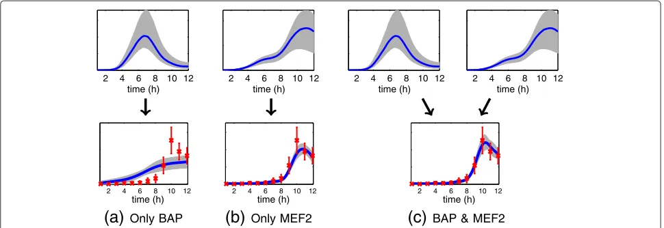
Figure 1Illustration of how two TFs can cooperatively regulate a gene.Results are shown for a putative target gene FBgn0036752 that is highly ranked as a joint target of the TFs Bagpipe (BAP) and Myocyte enhancer factor 2 (MEF2) by the proposed method. Red crosses show target gene expression data (12 time points) from [33] and blue lines show model predictions and associated credible regions. In the top row we show the activity profiles for each TF which are inferred during the training phase by fitting a regulation model on a network of known structure. In the bottom row we show the model fit during genome-wide scanning for this target gene. We show the target mRNA concentration profile inferred by fitted models of (a) regulation by BAP only, (b) regulation by MEF2 only and (c) regulation by BAP and MEF2. The candidate gene is confirmed as a joint target by independent ChIP-chip studies [12].

of 12 time points, thereby providing a practical tool for identifying context-specific regulatory targets. Our results show highly statistically significant enrichment for ChIP-confirmed bindings of the putative regulators in the same system and significantly better enrichment than compet-ing methods.

A confounding aspect when applying target prediction models for a limited number of regulators is the presence of TFs that are unknown or other unmeasurable influ-ences on the system. We show on simulated data that, despite the presence of such confounding influences, our model can reconstruct the influence of multiple regulators of interest. We also show how data from additional con-ditions can easily be incorporated to improve inference when available.

Results and discussion

Overview of the method

Our approach is based on three main components: i) the use of ODEs to model transcription, translation and mRNA/protein decay, ii) a known set of TFs that reg-ulate transcription and iii) data-driven inference of the model parameters and network structures by using a fully Bayesian statistical method [26]. To infer TF activities over time, which can be considered functional parameters in our model, we extend previously developed Gaussian pro-cess inference techniques [20,21] to the case of multiple TFs interacting through a non-linear regulation function. Here we provide a brief description of the methodology and introduce notation that is useful for the presentation of the results. A detailed description is given in Methods and the supplementary information.

Consider the following dynamical models for the time-evolution of mRNA and TF protein abundances driven by gene transcription and TF protein translation,

transcription dmj(t)

dt =bj+sjG

p1(t),. . .,pI(t);θj

−djmj(t).

This ODE model ties together the target gene mRNA concentrationmj(t), and the regulator TF protein activ-ities pi(t). The translation model then relates the TF protein activities to the corresponding TF mRNA levels fi(t),

translation dpi(t)

dt =fi(t)−δipi(t).

with rateδi. We assume that the main rate-limiting step in production of active TF protein is transcription. Thus the TF activity can be considered equivalent to the TF protein concentration. This is thought to be a reasonable assump-tion for TFs in theDrosophilaembryonic developmental system considered later [28] but in other systems TFs may be primarily regulated by post-translational modifi-cations. In theDrosophilasystem there is significant evi-dence for dimerisation of the TFs, see e.g. [29-32], but no evidence of regulation by other post-translational modifi-cations. In systems where TF activity is actively regulated by post-translational modification, e.g. through phospho-rylation by a signalling pathway, then the above translation model would not correctly model changes in the concen-tration of active TF protein in the nucleus. However, the modelling framework that we propose can still be applied by removing the translation equations and modelling the TF protein activity as a driving latent function; see [21] for examples of this approach to TF activity inference.

In many experiments the protein activities, pi(t), will be difficult or impossible to measure. These continuous-time profiles must be inferred along with the parameters

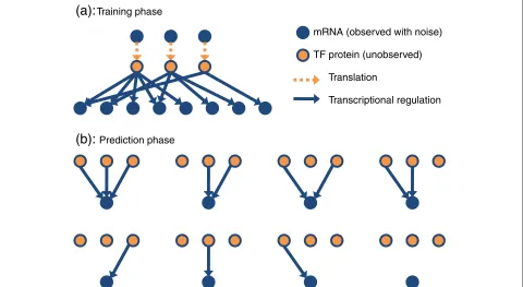
θ_j,dj,bj,sj and δi. Importantly, some individual param-eters in θ_j quantify the interactions between TFs and genes and the estimation of their values allows us to infer the network structure, i.e. to identify the subset of TFs that regulate the transcription of each gene. The full continuous-time mRNA functionsmj(t)andfi(t)are also unobserved. A typical set-up is that we have noisy obser-vations of these functions obtained at a set of discrete time points through gene expression analysis. Fitting the dynamical models to a biological system is carried out by the following two phases (see Figure 2):

1. Training phase: Here, we use the dynamical models to estimate the TF activities,pi(t), by using a small set oftraining genes. The approximate structure of this sub-network is assumed to be given so that for these genes the regulating TFs are known to some degree. All other model parameters are unknown and are inferred from the data. In this phase both the transcription model and the translation model are used to estimate the TFs. Observations associated with both the mRNA of the training genes and the TF mRNAs are required. The training phase could be carried out without the translation model in cases where TF protein activity is regulated by

post-translational modification. Extensive experimentation with artificial data reveals that, when appropriate, combining a translation model with TF mRNA observations greatly aids in estimation of the TF activities.

2. Prediction phase: Once the TF activities have been estimated, eachtest gene (for which the regulating

TFs are unknown) is processed independently and the parameters(θ_∗,d∗,b∗,s∗)are inferred. Here, only the transcription model is needed while the

translation model is irrelevant. This phase is applied on a genome-wide scale and aims to identify the regulating TFs for each test gene.

The above phases can be applied to a situation where prior biological knowledge provides information only about a small set of well-studied genes for which the reg-ulating TFs are known to some degree. These genes are treated as the training data that are used to infer the activ-ity profiles of the TFs. Typically, a full genome-wide list of targets of the TFs is unknown. This is the motivation behind the second phase which applies the trained mod-els for genome-wide prediction of network links between genes and TFs. An important property of the second phase is that it is trivially parallelizable which allows for fast computations. The algorithms for fitting the models are based on Bayesian probabilistic inference and details are given in the supplementary information.

We will illustrate our methodology using mesoderm development in embryonic Drosophila melanogaster. First, though, we create an artificial example that high-lights the difficulties inherent in inference of transcription networks directly from data.

Synthetic data

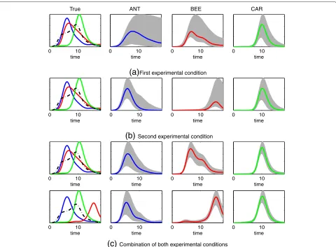
We consider an artificial gene network involvingfour tran-scription factors: ANT, BEE, CAR and UNK. We will sim-ulate data directly from our network, but when modelling the data we will only consider three of these transcrip-tion factors: ANT, BEE and CAR. This reflects a realistic scenario where there is an unacknowledged confound-ing transcription factor (UNK) affectconfound-ing our system. We simulated data associated with two experimental condi-tions. The data are short unevenly sampled time-series of 10 time points. In our first experimental condition there is considerable overlap between the TF concentrations of ANT and BEE as shown in Figure 3(a), while in the sec-ond experimental csec-ondition the overlap of BEE with ANT is far less (Figure 3(b)). In both experimental conditions there is considerable overlap between UNK and the three acknowledged TFs.

mRNA (observed with noise)

TF protein (unobserved)

Translation

Transcriptional regulation

(b):

(a):

Figure 2The proposed procedure for regulatory network inference.The procedure is divided into two phases: (a) The training phase involves learning the differential equation model parameters and inferring the unobserved TF protein activities on a sub-network of approximately known structure. By adopting a Bayesian inference procedure we can determine the posterior distribution over TF protein activities supported by the data. To close the system we place a Gaussian process prior distribution over the TF mRNA concentration functions [21]. (b) The prediction phase involves scoring all alternative regulation models for each putative target gene (2I_{models forITFs). During this phase we assume that TF activities have a} probability distribution given by the posterior distribution inferred during the training phase. The Bayesian evidence score is calculated for each regulation model and the posterior probability of any regulatory relationship of interest, such as TF–target gene associations, is determined by Bayesian model averaging.

the TF profiles. Specifically, to make the training phase more realistic we added 15% noise to the ground-truth network links in these 30 training genes. This resulted in 16 links between TFs and genes (in the initial ground-truth network structure) to change so that some of these links falsely became active and others were removed (i.e. from active they became inactive). Notice that this noise in the network links adds an extra model-mismatch in addition to the presence of the UNK TF which is not part of the model. In the prediction phase these pro-files were used to rank other potential targets of the TFs from the remaining 1000 genes. Full details on how the data have been generated are given in Methods, while the dataset is provided together with software that is available online.

To assess the predictive ability of the model with respect to the amount of information present in the data, we con-sider three experiments. In the first experiment only data from the first experimental condition are used, in the sec-ond experiment only data from the secsec-ond experimental condition are used, while in the third experiment all data from both conditions are considered.

Using data from one experimental condition

Here, we assume the synthetic mRNA data are produced by a single experimental condition, i.e. either the first or the second condition mentioned earlier. When consider-ing the first condition the true TF profiles for ANT, BEE, CAR and UNK are shown in the left plot of Figure 3(a) and the corresponding TF mRNA functions are shown in Additional file 1: Figure S1(a). The remaining three plots in Figure 3(a) show the TF activities estimated in the training phase by using 30 genes with approximately known network connectivity andunknownmodel param-eters. The coloured solid lines show the estimated means and the shaded areas represent 95% posterior credible regions around the estimated means. Plots showing how the model fits the mRNA data in the training phase are presented in Additional file 1: Figures S2 and S6 and all corresponding ODE parameters are shown in Additional file 1: Figures S9 and S10.

True ANT BEE CAR

0 10

time

0 10

time

0 10

time

0 10

time

(a)

0 10

time

0 10

time

0 10

time

0 10

time

(b)

0 10

time

0 10

time

0 10

time

0 10

time

0 10

time

0 10

time

0 10

time

0 10

time

(c)

Figure 3TF concentrations inferred by the model in the synthetic data.The plots in panel (a) (the four plots in the first row) illustrate the estimation of the TF activity using only the first experimental condition. The left plot shows the ground-truth TF activities that generated the observed data. In particular, the coloured solid lines show the three TFs, which were assumed to be known (blue: ANT, red: BEE, green: CAR) and the black dotted line displays the unknown factor UNK. The remaining three plots in panel (a) show the TFs estimated at the training modelling phase. Here, the coloured lines display the estimated means of ANT, BEE and CAR and the shaded areas show 95% credible regions. The plots in panel (b) display the exactly analogous plots with those of (a) with the difference that the second experimental condition was considered instead of the first. The plots in panel (c) illustrate the estimation of TFs by using simultaneously both experimental conditions. The plots in the first row of (c) display the estimates for the first experimental condition, while the plots of the second row display the estimates for the second experimental condition .

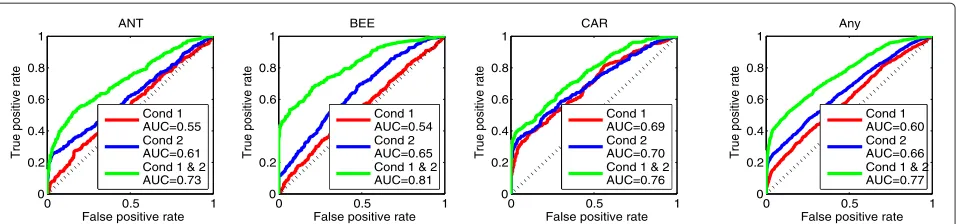
In particular, the estimation of these two TFs, shown in the second and third plot from the left in Figure 3(a), is rather uncertain (as indicated by the very large shaded area that represents uncertainty). Moreover, the fact that the profiles of these TFs overlap significantly with each other yields poor performance when predicting the net-work links. The ROC curves in Figure 4 show accuracy when predicting the individual TF links (first three plots from the left) and overall performance when predict-ing spredict-ingle links (last plot). In all panels the solid red line is the ROC curve associated with the performance of the model when using the first experimental condi-tion. Notice that for ANT and BEE the performance is only slightly better than random (diagonal dotted black

line). For CAR the performance is better since the pro-file of this TF overlaps much less with those of ANT and BEE.

0 0.5 1 0 0.2 0.4 0.6 0.8 1

False positive rate

True positive rate

ANT

0 0.5 1

0 0.2 0.4 0.6 0.8 1

False positive rate

True positive rate

BEE

0 0.5 1

0 0.2 0.4 0.6 0.8 1

False positive rate

True positive rate

CAR

0 0.5 1

0 0.2 0.4 0.6 0.8 1

False positive rate

True positive rate

Any AUC=0.73 Cond 1 AUC=0.55 Cond 2 AUC=0.61 Cond 1 & 2

Cond 1 AUC=0.54 Cond 2 AUC=0.65 Cond 1 & 2 AUC=0.81

Cond 1 AUC=0.69 Cond 2 AUC=0.70 Cond 1 & 2 AUC=0.76 Cond 1 AUC=0.77 AUC=0.60 Cond 2 AUC=0.66 Cond 1 & 2

Figure 4ROC curves for predicting the network connections in the synthetic data.Red curves show the results by using only the first experimental condition, blue curves show the results by using only the second experimental condition, while green curves correspond to the results when both experimental conditions are used. The diagonal black dotted line is the performance based on random prediction. The first three plots from the left show the ROC curves for predicting the individual TF links and the last plot shows the overall performance, i.e. for predicting any link .

We now consider a second series of observed mRNA measurements associated with an alternative simulated experimental condition comprising a perturbation of the biological system that better disambiguates the two (pre-viously overlapping) TFs in terms of their influence in gene transcription. We first use only these new data instead of the data associated with the first experi-mental condition. This alternative perturbation changes significantly the protein activity for BEE as shown on the left plot in Figure 3(b), while ANT, CAR and UNK are assumed to behave similarly to the first experimen-tal condition. The estimated TFs are shown in the plots of the remaining three columns of Figure 3(b) and model fits in the training mRNA data for this second condi-tion are plotted in Addicondi-tional file 1: Figures S3 and S7 and all associated ODE parameters are shown in Addi-tional file 1: Figures S11 and S12. The blue ROC curves in Figure 4 show predictive performance when using this second experimental condition. As the blue curves indicate, the performance now improves compared to the results obtained by using the first condition (red curves). This is expected since the second condition dis-ambiguates more efficiently the TF activities than the first condition. In the next section we will see that the performance can be further improved when the models are fitted simultaneously to data from both experimental conditions.

Combining the data from both experimental conditions In our third experiment we fit the models using all data from both experimental conditions. Figure 3(c) shows the TFs that generated the mRNA data for both experimen-tal conditions (plots in the first column from the left) and the estimated TFs (plots in the remaining three columns). Each row of Figure 3(c) corresponds to each of the two conditions. Model fits in the training mRNA data are plotted in Additional file 1: Figures S4 and S8 and all asso-ciated ODE parameters are shown in Additional file 1: Figures S13 and S14.

Including data from both experimental conditions allows for a more confident estimation of the TF profiles. To see this, we can contrast the second up to fourth plots in the first row of Figure 3(c) with the corresponding plots of Figure 3(a)-(b). The credible regions when simultane-ously using both experimental conditions are significantly smaller, which implies higher confidence.

Furthermore, we obtain a significant increase in the pre-dictive performance when identifying network links. As the green coloured ROC curves in Figure 4 reveal, the performance when predicting single network links is sig-nificantly improved. Finally, we can exploit the ability of the model to predict a simultaneous regulation of the tar-get gene by two or more TFs. Additional file 1: Figure S5 displays the predictive ROC curves for all three TF pairs in this example.

Drosophiladata

2 4 6 8 10 12 time (h)

2 4 6 8 10 12

time (h)

2 4 6 8 10 12

time (h)

2 4 6 8 10 12

time (h)

2 4 6 8 10 12

time (h)

2 4 6 8 10 12

time (h)

2 4 6 8 10 12

time (h)

2 4 6 8 10 12

time (h)

2 4 6 8 10 12

time (h)

2 4 6 8 10 12

time (h)

TIN

BIN

TWI

BAP

MEF2

Figure 5The estimated TF activities and predicted TF mRNAs from the training modelling phase inDrosophiladata.The five plots in the first row display the estimated TFs of the third replica. Each blue solid line represents an estimated mean TF activity and the shaded area represents 95% credible regions around the mean. The five plots in the second row display the predicted TF mRNAs (blue solid lines and shaded areas) together with the observed data represented by red crosses (means) and vertical lines (two-standard deviations around the means provided by the microarray preprocessing stage) .

used in final training with only noise from preprocess-ing included in the model. Figure 5 shows the inferred profiles for all five TFs (first row) together with the corre-sponding predicted TF mRNAs (second row) for the third replica of the time-series. The TF profiles and predicted TF mRNAs for the remaining two replicas are shown in Additional file 1: Figure S15. Model fits in the training mRNA target gene data are shown in Additional file 1: Figure S18 (showing genes included in final training) and Additional file 1: Figure S19 (showing genes excluded from final training) in the supplementary information while ODE parameters are shown in Additional file 1: Figures S20 and S21.

Prediction of network connections

Once the TF activities have been estimated, we use the model to predict the regulator TFs for a set of 6003 test genes which exclude the 92 genes used in the training phase. A web-based browser that displays how the model fits the mRNA data of test genes is available online at [34]. Full posterior probabilities of all alternative models for all test genes are included in Additional file 2. This set includes all genes in the data that are not classified as weakly expressed according to the criterion explained previously [20]. We followed an approach to evaluation of predictive performance similar to one described in [20]. A number of predictions is evaluated by considering for each

50 100 200 400 800 1600 3200 0

20 40 60 80 100

# of top predictions

Enr

ichment (%)

*** _***

*** _***

*** _{*** ***} *** _***

*** _***

*** _***

***

** ****** ****** ***_*** ***_*** ******

Posterior−32 Posterior−2 ML−Baseline Inferelator Uniform prior

50 100 200 400 800 1600 3200 0

20 40 60 80 100

# of top predictions

Enr

ichment (%)

** _{*** *** ***}

*** *** _*** ** *** _{*** *** *** ***}

***

* *** *** *** *** * _{* ** *** ***}

***

Posterior−32 Posterior−4 ML−Baseline Inferelator Uniform prior

(a)

(b)

Table 1 Link-specific ChIP evaluation bootstrap results

Predicting regulation by single TFs

Top 50 Top 100 Top 200

P32 P2 ML Inf P32 P2 ML Inf P32 P2 ML Inf

P32 *** * P32 ** ** P32 ** **

P2 *** ** P2 + *** *** P2 *** **

ML ML ML

Inf Inf Inf

Top 400 Top 800 Top 1600

P32 P2 ML Inf P32 P2 ML Inf P32 P2 ML Inf

P32 * *** P32 + *** P32 * ***

P2 ** *** P2 * *** P2 * ***

ML * ML *** ML ***

Inf Inf Inf

Top 3200

P32 P2 ML Inf

P32 *** *** ***

P2 * ***

ML ***

Inf

Predicting regulation by TF pairs

Top 50 Top 100 Top 200

P32 P4 ML Inf P32 P4 ML Inf P32 P4 ML Inf

P32 ** + P32 * . P32 + *

P4 ** + P4 * + P4 + *

ML ML ML

Inf . Inf Inf

Top 400 Top 800 Top 1600

P32 P4 ML Inf P32 P4 ML Inf P32 P4 ML Inf

P32 * ** P32 + *** P32 **

P4 + ** P4 * *** P4 ** * ***

ML ML . ML +

Inf Inf Inf

Top 3200

P32 P4 ML Inf

P32 *

P4 *** ** ***

ML * ***

Inf

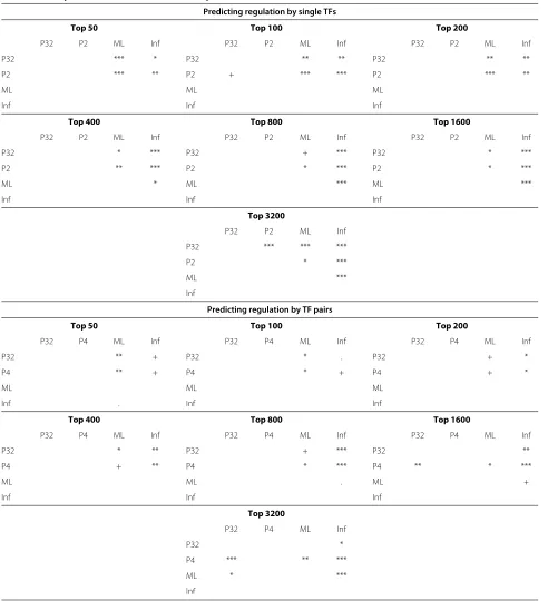
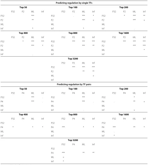
The results of 100,000-fold bootstrap resampling of the data set of observed genes to assess significance of differences in ranking method performance. The methods studied are: P32 = Posterior-32 method, P2 = Posterior-2 method, P4 = Posterior-4 method, ML = ML Baseline method, Inf = Inferelator. For each pair of methods, the marks in the tables show how often the method on the corresponding row dominated the one on the corresponding column. The marks are interpreted as follows: ‘.’: >80%dominance, ‘+’:>90%dominance, ‘*’:>95%dominance, ‘**’:>99%dominance, ‘***’:>99.9%dominance, ‘-’: comparison not applicable.

gene a predicted set of regulators correct if all TFs in the set had evidence of binding within 2000 base pairs of the corresponding gene in the ChIP-chip data in [12]. Differ-ent methods can be compared based on the corresponding

similar evaluation using TF-gene links in the Drosophila Interaction Database (DroID) [35]. This database in not specific to development and may thus include links that are not active in our data. We only include the 5521 test genes with some predicted TF regulators in the database. We compare two variants of our proposed method to a maximum-likelihood-based baseline method, the Infere-lator 1.1 [15] and a simpler sparse regression approach (see Methods).

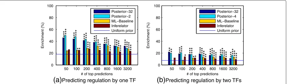
In the plots of Figure 6, we consider inferring single TF and TF-pair regulators with ChIP evaluation. The single-TF ranking is constructed by computing for each gene the marginal posterior probability of the event that a cer-tain TF is a regulator. Since we have five TFs, there are five probabilities of this type for each gene. We compute the posterior probabilities in two ways: either averag-ing over all models weighted by their marginal likelihood (“Posterior-32”) or using just the selected and null mod-els (“Posterior-2”). The resulting 5 × 6003 probabilities are sorted in decreasing order and Figure 6(a) displays the enrichment results at different cutoffs of this list. The predictions of both these methods are significantly bet-ter than random (p < 0.01 or less in all cases using tail probability in a hypergeometric distribution) and clearly outperform the maximum likelihood baseline and the Inferelator. We also carried out empirical bootstrap tests for each pair-wise comparison of methods which confirm that the proposed methods outperform the other methods statistically significantly in most cases (see Table 1).

For the TF-pair regulator rankings, we compute the marginal posterior probabilities for all possible pairs of TFs for each gene. The counterpart of Posterior-2 now

includes four models: the pair, both partners individually and the null, and is denoted by “Posterior-4”. Otherwise the ranking lists are computed exactly as in the case of single-TF regulators but now for the 10 × 6003 possi-ble TF-pair models. Figure 6(b) displays the results. The figure again shows statistically highly significant enrich-ment of binding of predicted regulators near the corre-sponding target genes. The enrichment is lower than it was for single-TF predictions, which is expected since the task of identifying regulating pairs of TFs is harder but may also be partly due to an increased number of false negatives in the validation data. The Bayesian methods based on posterior probabilities are consistently more accurate than the maximum likelihood baseline. In most cases the more restricted set of models seems to yield better results. Nevertheless, there are some TFs for which the opposite is true, as illustrated by the cor-responding results, broken down for each TF, that are shown in Additional file 1: Figures S16 and S17. This may be because the more restricted posterior probabili-ties are less sensitive to misspecification of prior proba-bilities of network links. Currently all TFs are assumed to regulate every gene with prior probability 0.5, which is unrealistic. Unfortunately it is nontrivial to construct better alternatives without significant extra information because the TFs are heavily correlated. We did not wish to use the ChIP data for constructing such a prior since this was required as independent data for validating the results.

We also compute thea posteriorimost probable regu-lator model for each gene, which we refer to as the maxi-mum a posteriori (MAP) model. Figure 7 shows results of

200 400 800 1600 3200 6003 0

20 40 60 80

# of top genes

Enrichment (%)

*** *** *** _***

*** _*** ** ***

***

MAP−32 ML−Baseline Regression

Inferelator (only for 6003 genes) Uniform prior

200 400 800 1600 3200 6003 0

20 40 60 80

# of global top genes Enrichment (%) *** ***

*** *** _***

***

*** *** *** _{*** ***}

***

** *** ***

MAP−32 ML−Baseline Regression

Inferelator (only for 6003 genes) Uniform prior

(a)

(b)

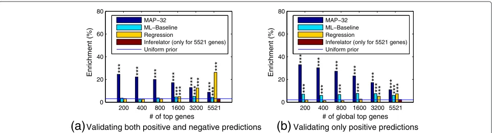
the ChIP evaluation based on the MAP regulator configu-ration for every gene, ranked by the posterior probability of this most probable model. Because there is no clear way to rank the genes with the Inferelator, the accuracy is only shown for the complete list of all genes. Additionally we compare the results against a more straightforward sparse regression method (“Regression”; see Methods for details). Figure 7(a) displays results for full validation of both positive and negative predictions. The results of the pro-posed method are statistically very significantly better than random, while the maximum likelihood baseline and the Inferelator are no better than random guessing. The regression method does poorly at first but ends with a much higher accuracy than all others. The main reason for this is that it makes a higher fraction of negative predictions; all other methods make many fewer predic-tions for genes being unregulated by all TFs while such

cases are fairly common based on our validation data. This behaviour is expected for the probabilistic method, which has a uniform prior over regulating TF combina-tions. Under this prior, the prior probability for a gene to be unregulated is only 1/32. If a more sensible prior is used, for example, by considering the empirical prior from the binding frequencies in the validation data, the pro-posed method can attain even higher accuracy than the regression method (results not shown). According to the bootstrap testing, the proposed method is statistically sig-nificantly better than the alternatives in all cases except regression with≥ 3200 top predictions (p < 0.01; see Table 2 for full results).

Because of frequent non-functional binding [11], it makes sense to ignore additional bound TFs. In this case negative predictions cannot be validated, only posi-tive ones. Figure 7(b) shows the validation results in this

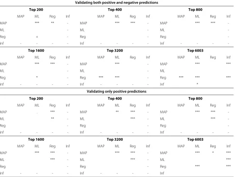
Table 2 Full model ChIP evaluation bootstrap results

Validating both positive and negative predictions

Top 200 Top 400 Top 800

MAP ML Reg Inf MAP ML Reg Inf MAP ML Reg Inf

MAP *** ** - MAP *** *** - MAP *** ***

-ML - ML - ML

-Reg + - Reg - Reg

-Inf - - - - Inf - - - - Inf - - -

-Top 1600 Top 3200 Top 6003

MAP ML Reg Inf MAP ML Reg Inf MAP ML Reg Inf

MAP *** *** - MAP *** - MAP *** ***

ML - ML - ML

Reg * - Reg *** *** - Reg *** *** ***

Inf - - - - Inf - - - - Inf *

Validating only positive predictions

Top 200 Top 400 Top 800

MAP ML Reg Inf MAP ML Reg Inf MAP ML Reg Inf

MAP . *** - MAP ** *** - MAP *** ***

-ML ** - ML *** - ML ***

-Reg - Reg - Reg

-Inf - - - - Inf - - - - Inf - - -

-Top 1600 Top 3200 Top 6003

MAP ML Reg Inf MAP ML Reg Inf MAP ML Reg Inf

MAP *** *** - MAP *** *** - MAP *** * ***

ML *** - ML *** - ML ***

Reg - Reg - Reg *** ***

Inf - - - - Inf - - - - Inf

case. Genes with a MAP model with no regulation were ignored because they would all be judged as “correct” here, biasing the accuracy results. The figure again shows sta-tistically significant enrichment of binding of predicted regulators near the target genes. The proposed Bayesian method based on posterior probabilities is clearly more accurate than the maximum likelihood baseline and also more accurate than the regression method in all cases. According to the bootstrap testing, the proposed method is statistically significantly better than the alternatives in all cases except maximum likelihood baseline 200 top pre-dictions (p < 0.01, exceptp < 0.05 for regression with 6003 top predictions; see Table 2 for full results). The computation times of the different alternatives are listed in Table 3.

Similar evaluation for DroID validation is shown in Figures 8 and 9. In Figure 8 the relative order of the meth-ods is mostly the same as in Figure 6, but the percentage enrichments of all methods are significantly lower. This may be due to incompleteness of the DroID database. The number of annotated TF-gene interactions in DroID is roughly similar to the number of genes with ChIP binding for TWI, but much lower for all other TFs. The num-ber of genes with more than one regulator is even more significantly lower in DroID. As the ChIP data was gath-ered using the same protocol for all TFs, it seems more likely to contain balanced information for all TFs. Never-theless, the most probable regulator combination results in Figure 9 show very high accuracy for our MAP method, which is very clearly superior to all other methods, except regression when using the full list of genes. Bootstrap testing results are presented in Tables 4 and 5.

Parameter estimates

The protein degradation rates and the corresponding pro-tein half-life estimates from the model are presented in Table 6. The estimates are unusually short for proteins in general, but they are in line with recent research demon-strating that Twist homologue has a very short half-life in the mouse [36]. As other studied TFs are from the same protein family, it is plausible they could share simi-lar half-lives. Cell division also contributes to the effective degradation rate and it is also possible that diversification during development can lead to a higher effective decay rate since the proportion of cells with tissue-specific TF

Table 3 Running times

MAP-32 Baseline Regression Inferelator

5911.50 2236.36 0.96 0.25

Running computer times (in seconds) of different methods for scoring all possible 32 models (combinations of five TFs) in a single target gene (out of the 6003 genes) in theDrosophiladata.

activity reduces over time. These effects will also increase the effective target mRNA degradation rates.

Discussion

It may be thought that a typical short time-series expres-sion dataset contains only very limited information about the structure of a GRN. In a meta-analysis of methods proposed in the DREAM 2 competition [37], the authors in [4] found time-series data to be much less informative for network inference than data from a similar number of perturbation experiments. However, in the datasets con-sidered there many of the time-series experiments are rather uninformative about expression changes given the level of noise in the data and uninformative selection of sampled time points. We would argue that the success of a method for analysis of time-series data will depend greatly on how informative the profiles of the regulatory species are. In our synthetic example we clearly demonstrated how inference is sensitive to confounding by highly sim-ilar temporal profiles of regulating TFs, so it is certainly desirable to have access to data from diverse experimental conditions where available. Yet with an animal system the available perturbations may be severely limited and the wild-type under normal conditions is of great interest for understanding healthy function. Methods for learning the structure of a regulatory network from one or a few short time course experiments are of great practical importance for uncovering a condition-specific GRN.

(a)

(b)

0 20 40 60 80

# of top predictions

Enr

ichment (%)

*

***_*** *** *** *** *** _*** *** *** *** _{*** ***}

** *** *** *** *** * _* *** *** *** _{*** ***}

Posterior−32 Posterior−2 ML−Baseline Inferelator Uniform prior

50 100 200 400 800 1600 3200 0

5 10 15 20

# of top predictions

Enr

ichment (%)

* ** _{** ***}

**

** *** *** *** ***

***

**** ****** ****** _******

Posterior−32 Posterior−4 ML−Baseline Inferelator Uniform prior

Figure 8Enrichment of confident regulator predictions for DroID interactions.Similar to Figure 6 but using DroID database TF-gene interactions instead of ChIP binding for validation .

challenging task that is not addressed in [18] and [20]. Additional information, even just independent estimates of decay rates of different transcripts, would certainly make the task easier, as demonstrated in [38] and also our results on synthetic data.

The Inferelator is an effective method for target iden-tification which also uses a non-linear regulation model that accounts for regulation by multiple TFs [15]. The Inferelator is applicable more generally since it uses less prior information about the system than we are assuming. Two important assumptions were made in the analy-sis of the Drosophila data; we assumed knowledge of a well-characterised sub-network of the GRN, which is used to learn the TF activity profiles during the training phase, and in the present application we restrict our-selves to models of activation. Our results demonstrate improved performance over the Inferelator but it should be acknowledged that we are solving a more restricted class of problem. Our method is also much more com-putationally demanding (see Table 3); it is applicable to genome-wide scanning for a small set of TFs but would not be applicable for a very large set of regulating TFs in the current implementation. Nevertheless, our results

demonstrate that the inclusion of additional domain knowledge or prior assumptions, where available, can improve performance over more general methods. Prob-abilistic modelling provides a useful framework for the inclusion of such prior knowledge.

Inference of continuous-time TF activity profiles from short time-series is an ill-posed problem. We resolve this through introduction of a Gaussian process prior that effectively assumes smoothness of the underlying func-tions [21]. While this assumption appears reasonable for the TFs studied here, there are situations where the TF is activated very rapidly through signalling, e.g. in a sen-sory GRN [39]. In these situations an alternative model better suited for fast transitions such as that presented in [40] may be preferable. Alternatively, the Gaussian pro-cess could be transformed to provide a sharper switching behaviour by passing it through a sigmoidal non-linearity (cf. Gaussian process classification [41]) and the current inference methodology would remain applicable.

Carrying out Bayesian inference over non-linear sys-tems with functional parameters is very challenging. For parameter inference we have made use of state-of-the-art methods for Markov chain Monte Carlo (MCMC) over

(a)

(b)

200 400 800 1600 3200 5521

0 20 40 60 80

# of top genes Enrichment (%) *** *** *** _***

***

***

****** *** ***

***

***

MAP−32 ML−Baseline Regression

Inferelator (only for 5521 genes) Uniform prior

200 400 800 1600 3200 5521

0 20 40 60 80

# of global top genes

Enrichment (%)

*** _***

***

***

***

***

*** *** *** *** ****** ******

MAP−32 ML−Baseline Regression

Inferelator (only for 5521 genes) Uniform prior

Table 4 Link-specific DroID evaluation bootstrap results

Predicting regulation by single TFs

Top 50 Top 100 Top 200

P32 P2 ML Inf P32 P2 ML Inf P32 P2 ML Inf

P32 *** P32 . *** * P32 * *** **

P2 ** P2 *** + P2 *** +

ML ML ML

Inf * Inf * Inf .

Top 400 Top 800 Top 1600

P32 P2 ML Inf P32 P2 ML Inf P32 P2 ML Inf

P32 * *** *** P32 *** *** *** P32 *** *** ***

P2 *** * P2 *** ** P2 *** ***

ML ML ML *

Inf . Inf Inf

Top 3200

P32 P2 ML Inf

P32 *** *** ***

P2 ** **

ML +

Inf

Predicting regulation by TF pairs

Top 50 Top 100 Top 200

P32 P4 ML Inf P32 P4 ML Inf P32 P4 ML Inf

P32 *** . P32 *** P32 *

P4 *** . P4 *** . P4 . ** +

ML ML ML

Inf Inf . Inf +

Top 400 Top 800 Top 1600

P32 P4 ML Inf P32 P4 ML Inf P32 P4 ML Inf

P32 P32 P32

P4 * * * P4 *** * * P4 *** ** *

ML ML ML .

Inf Inf Inf *

Top 3200

P32 P4 ML Inf

P32

P4 *** ** **

ML +

Inf *

Same as Table 1 but for DroID evaluation.

functional degrees of freedom [42]. We have developed a novel fast method for calculating the Bayesian evidence score that allows us to carry out genome-wide model scor-ing (see supplementary information). Our method is very easily parallelizable within the prediction phase and can

therefore be considered a practical contribution to the functional genomics toolkit.

Table 5 Full model DroID evaluation bootstrap results

Validating both positive and negative predictions

Top 200 Top 400 Top 800

MAP ML Reg Inf MAP ML Reg Inf MAP ML Reg Inf

MAP *** *** *** MAP *** *** *** MAP *** *** ***

ML ML ML . .

Reg Reg Reg

Inf Inf Inf

Top 1600 Top 3200 Top 6003

MAP ML Reg Inf MAP ML Reg Inf MAP ML Reg Inf

MAP *** *** *** MAP *** *** MAP

ML ** ML *** ML

Reg ** Reg *** *** Reg

Inf Inf Inf

Validating only positive predictions

Top 200 Top 400 Top 800

MAP ML Reg Inf MAP ML Reg Inf MAP ML Reg Inf

MAP *** *** *** MAP *** *** *** MAP *** *** ***

ML ** + ML *** * ML *** ***

Reg Reg Reg

Inf Inf + Inf *

Top 1600 Top 3200 Top 6003

MAP ML Reg Inf MAP ML Reg Inf MAP ML Reg Inf

MAP *** *** *** MAP *** *** *** MAP

ML *** *** ML *** *** ML

Reg Reg *** Reg

Inf Inf Inf

Same as Table 2 but for DroID evaluation.

analysis of expression data can be combined with evi-dence from complementary sources (ChIP data, in situ expression data, sequence motifs) to identify a confident regulatory network structure. For example, [20] show how the accuracy of model-based prediction improves greatly when additional evidence from spatial expression data is considered. The Bayesian framework presented here pro-vides a very natural means for integrating other sources of data or prior knowledge for network inference. For example, it would be straightforward to associate alterna-tive regulatory structures (e.g. those in Figure 2(b)) with different prior probabilities derived from ChIP-chip bind-ing patterns. These priors could be used to re-weight the Bayesian model averaging scheme used to calculate the probability of network structures. We do not pursue this approach here because we want independent ChIP-chip validation of our method’s performance. Alternatively,

given time-series ChIP data, one could include binding observations directly in the model. This would have the advantage that one could model measurement errors for both the expression and ChIP experiments.

Conclusion

Table 6 Inferred protein degradation rates

Degr. (1/h) half-life (h) TIN (0.81, 1.19, 1.66) (0.42, 0.58, 0.86)

BIN (0.62, 0.80, 1.08) (0.64, 0.87, 1.12)

TWI (3.79, 4.62, 5.79) (0.12, 0.15, 0.18)

BAP (3.08, 5.41, 8.27) (0.08, 0.13, 0.23)

MEF2 (0.57, 0.80, 1.67) (0.41, 0.86, 1.20)

Inferred protein degradation rates (first row) for the five TFs and the

corresponding estimates for the half-life of each protein (second row). Recall that the formula for the half-life islog(2)/δwhereδis protein degradation rate. Each triple(a,b,c)of values corresponds to 5% percentile, median and 95% percentile.

of TF protein activity given a small subnetwork of mostly known structure. Subsequently we score alternative tar-get gene regulation models to make genome-wide tartar-get predictions. By using a fully Bayesian procedure we are able to automatically balance model complexity with data fit when scoring alternative models. Our method is readily parallelizable in the prediction phase, making it a practical tool for genome-wide network inference. On artificial data we showed that our method is able to cope with the existence of unknown regulating TFs that are not modelled and we showed that data from more diverse experimental conditions can help disambiguate between TFs that have similar profiles in a single condi-tion. However, as our Drosophila example shows, even a single wild-type time course can be highly informative about the underlying regulatory network if the TFs of interest are changing over time. By combining the model predictions with other independent sources of evidence, e.g. from ChIP and spatial expression patterns, it will be possible to identify a confident condition-specific regulatory network.

Availability

Software and a web-based browser displaying results in the Drosophila experiment are both available online at [34].

Methods

Dynamical models

The transcription and translation equations are ordinary differential equations (ODEs) having the general form given in the beginning of the Results section. The response function G(·) non-linearly transforms the TF protein activities{pi(t)}Ii=1, and has the following sigmoidal form:

G(p1(t),. . .,pI(t);wj,wj0)=

1

1+e−wj0−iI=1wjilogpi(t) .

Here, the I-dimensional real-valued vector wj =

wj1. . .wjI

stores the interaction weights between the

jth target gene and theI TFs. These interaction weights quantify the network links so that when wji = 0 the link between thejthgene and theithTF is absent. When wji is negative or positive the TF acts as a repressor or activator respectively.wj0is a real-valued bias parameter. The set of scalar parametersθ_j in the response function G(·)is defined to beθj = {wj,wj0}. Since the transcrip-tion ODE model is linear with respect to mj(t), it can be solved explicitly as shown in the supplementary infor-mation. The above transcription ODE model generalizes previous single-TF models that were used to estimate the concentration function of a single latent TF [18,21,43]. While a sigmoidal form for the response functionG(·)was considered in all our experiments, our algorithms could easily be adapted to handle different forms forG(·).

Furthermore, the simple linear translation equation can be solved explicitly as shown in the supplementary infor-mation. Finally, the parameters{θ_j,dj,bj,sj,δi}are model parameters in the ODEs which need to be estimated under the constraint that {dj,bj,sj,δi} attain non-negative real values, whileθ_j = {wj,wj0}can attain both positive and negative real values. When we search for TFs that act only as activators,wjis constrained to be non-negative.

A more detailed description of the ODE models is given in section 2 of the supplementary information.

Training modelling phase

The dynamical models contain a set of unknown quanti-ties: the transcription model parameters {θ_j,dj,bj,sj}Jj=1, where J is the number of target genes, the unobserved TF protein activities{pi(t)}Ii=1and the TF protein degra-dation rates {δi}Ii=1. To estimate these quantities in the training modelling phase we consider a Bayesian prob-abilistic approach. More precisely, the observed mRNA data are used to construct likelihood functions that explain how the data are generated from the dynamical models. Together with the mRNA data for each train-ing gene j we also have a binary vector xj ∈ {0, 1}I that specifies the regulatory network structure for that gene so that xji = 1 indicates the presence of the link between the gene and the i TF, while xji = 0 indi-cates the absence of the link. Prior distributions are assigned to all unknown quantities. The prior over each protein activity pi(t) was defined through the transla-tion ODE and the placement of a suitable prior on the TF mRNA function, fi(t), through the use of Gaussian processes; see e.g. [41]. Bayesian inference in the train-ing modelltrain-ing phase was performed by Markov chain Monte Carlo (MCMC) techniques [44] where all the above unknown quantities were inferred using suitable MCMC updates.

Prediction modelling phase

The prediction phase involves independently processing each test gene and probabilistically predicting its regulat-ing TFs. Let∗denote a test gene so thaty_∗is the associated vector of observed mRNA measurements. This gene can be regulated by any combination ofITFs. Letx∗∈ {0, 1}I be the binary vector that indicates the subset of the TFs that regulate gene ∗which takes 2I possible values. To infer the network links, it suffices to compute the posterior probability for each value of the discrete random variable x∗. Using Bayes’ rule this probability is

p(x∗|y_∗,Y)= p(y∗|x∗,Y)p(x∗|Y)

xp(y∗|x,Y)p(x|Y)

, (1)

whereYindicates the data used in the training modelling phase. To obtain the above, we need to compute the pre-dictive density p(y_∗|x∗,Y) for any possible combination of regulating TFs, i.e. any value of x∗, together with the associated probabilitiesp(x∗|Y). Whilep(x∗|Y)could be computed by the frequencies of the known connectivity vectors in the training genes, this is unreliable since the small set of training genes may not be representative about the prior distribution of links between TFs and genes. Therefore, we set these probabilities to uniform values so that the posterior probability in Equation (1) becomes proportional to its predictive density value p(y∗|x∗,Y). This latter quantity is intractable since it requires an inte-gration over the parameters(θ_∗,d∗,b∗,s∗). We approxi-mate it using a novel fast approximation to a marginal likelihood, described in detail in section 4.1 in the supple-mentary information, that follows ideas similar to Chib’s approximation [45].

Given the estimated probabilitiesp(x∗|y_∗,Y), withx∗∈

{0, 1}I, any query related to the regulating TFs of target gene ∗can be answered. For instance, in the results we made use of the following quantities:

• Maximum a posteriori (MAP) network configuration: This is the most probable settingxMAP_∗ for the network links obtained by

xMAP_∗ =arg max

x∗ p(x∗|y∗,Y). (2)

• Marginal probability of a single link: The link between the test gene and theithTF is present with posterior probability

p(x∗i=1|y∗,Y)=

x∗:x∗i=1

p(x∗|y_∗,Y). (3)

Similarly we can compute the marginal probability

p(x∗i=1,x∗j=1|y∗,Y)for a pair of links.

A more detailed description of the prediction mod-elling phase is given in section 4 of the Supplementary Information.

The “Maximum Likelihood Baseline” method

This method, that was used in the experiments in Drosophila, follows exactly the same structure as the Bayesian approach with the following two differences. Firstly, the model parameters (such as kinetic parameters in the ODEs) were not treated using a Bayesian man-ner and instead they were obtained based on maximum likelihood which provides point estimates. Secondly, each protein function,pi(t), was deterministically estimated by the translation ODE model and by setting the driving TF mRNA function,fi(t), to a piece-wise linear interpo-lation function computed from the TF mRNA observa-tions. Apart from the above differences, prediction using the baseline method is done exactly analogously to the Bayesian case.

The “Regression” method

In the experiments inDrosophila(Figure 7), we made use of a simple method for predicting the regulators of a target gene based on linear regression that predicts the mRNA of target gene from the TF mRNA. In particular, for a target genejthis linear model is

mjn= I

i=1

wjifin+wj0+n, ∀n,

where mjn is the observed mRNA of the target gene at timetn, {fin}I_i=1 the corresponding observed TF mRNA values,({wji}I_j=1,wj0) are parameters to be inferred and _n is Gaussian noise. Notice that,{wji}Ij=1are interaction weights andwj0is a bias parameter. Network inference in this linear model reduces to finding the non-zero interac-tion weights. This problem would typically require sparse optimization methods based on1regularization as con-sidered in [46]. However, in our case such algorithms are not needed since the number of TFs is small (I = 5) and hence we can enumerate all possible 32 regression mod-els and select the best model using cross-validation. In the results reported in Figure 7, we firstly computed for each gene the MSE scores on held-out data (using 12-fold cross validation) for all 32 models. Subsequently, we selected the model with the smallest MSE score for each gene and finally we ranked all genes based on the latter MSE scores (in ascending order) to produce the rankings shown in Figure 7.

Application of the Inferelator 1.1

new data. We set each gene in its own cluster but other-wise used the default settings. We interpreted the maxi-mum of the absolute values|βi|of all weights correspond-ing to a specific regulator alone or in combination with another as the counterpart of the posterior probability for ranking the predictions. For pairs, the corresponding value was max(|β3|, min(|β1|,|β2|)), whereβ1andβ2are the weights of the components(x1,x2)of the pair andβ3 is the weight of min(x1,x2)(see Eq. (6) in [15]). Combin-ing information from independent and interaction terms like this significantly increased the performance of the method. Ranking by|β_i|was also used in DREAM3 chal-lenge submission of the Inferelator team [47].

Preprocessing of theDrosophiladata

As previously described [20].

Training set for theDrosophiladata

The training set was constructed from the training set of 310 ChIP cis-regulatory modules (CRMs) collected in [12] (Additional file 1: Table S8). The modules were mapped to genes using the CRM activity database in [12] (Additional file 1: Table S4). Multiple CRMs for a gene were combined by taking the union of detected binding. Weakly expressed genes as defined in [20] were excluded, leaving a training set of 92 genes with well-characterised TF binding profiles.

Bootstrap significance testing of ranking method performance differences

100, 000-fold bootstrap resampling was used to assess sta-tistical significance of performance differences between different ranking methods. For each fold, the set of testing genes was resampled with replacement from the full set of 6003 genes. Top-ranked predictions within the resampled set were evaluated as usual and the fraction of folds where each method outperformed each other was tabulated.

Reduced training set for theDrosophiladata using a robustified model

Since in the Drosophila data the target genes can be influenced by unknown factors that are not part of the model, we considered a robustified training procedure that filtered out genes not explained by the model. This procedure allowed us to reduce the initial set of 92 genes to 25 genes and was carried out as follows. Firstly, we performed a training phase using all 92 genes so that the likelihood functions had both preprocessing noise vari-ances and additive gene-specific adaptive varivari-ances. Then, genes having large inferred adaptive variances, which indi-cates that these genes cannot be explained well by the five-TF model, are excluded so that finally a subset of 25 genes was retained. Then, the whole training phase was repeated using only the selected genes and without the

additive variances this time. The selection involved setting a threshold, which was set to 0.01, so that genes hav-ing estimated adaptive variance larger than this threshold were excluded. The threshold value was chosen to be smaller than the average value of the preprocessing vari-ances, which represent estimates of the actual observation noise in the gene expression measurements.

Robust fitting was also used in the prediction phase so that each test gene was fitted using a likelihood function in which the variance parameter was the sum of a fixed pre-processing noise variance and an adaptive variance. Again this allowed us to compensate for the model mismatch and the presence of other confounding factors which, while they could regulate the gene expression, are not part of the model. More details on the robustified fitting are given in Section 3 and 5.2 of the Supplementary Material.

DroID validation

We downloaded the TF-gene interaction database from DroID (http://www.droidb.org, release 2011 11). Genes with no interactions in the database were excluded from the validation to avoid possible problems due to annota-tion incompatibilities.

Generation of the synthetic data

We generated synthetic mRNA time-series data that cor-respond to 1030 target genes and four transcription fac-tors: ANT, BEE, CAR and UNK. The TF activities are depicted in the first column of Figure 3(c). For both experimental conditions, the TF activities have been gen-erated by simulating the translation ODE equation by assuming certain profiles for the TF mRNA functions,

{fi(t)}4_i=1, which were chosen to have the profiles shown in Additional file 1: Figure S1, and with protein degradation rates 0.994, 0.945, 0.640, 1.2 for the four TFs respectively. ANT, BEE and CAR are assumed to be known factors for which observations of their TF mRNA activities are available. UNK is assumed to be a confounding factor whose presence and origin is not known. Given these TF mRNA functions,{fi(t)}3i=1, noisy “observations” were obtained at ten non-uniformly spaced time points,tk ∈

{0, 1, 2, 3, 5, 7, 9, 11, 14, 18}, by adding zero-mean Gaussian noise with variance 0.025fi(tk)to the valuefi(tk). Negative values were truncated to zero.

Table 7 mRNA degradation rates

mRNA degrad. rates Protein degrad. rates (5%,median,95%) (ANT, BEE, CAR, UNK) (0.123, 0.610, 4.807) (0.994, 0.945, 0.640, 1.200)