Validating protein structure using kernel density estimates

This is a repository copy of

Validating protein structure using kernel density estimates

.

White Rose Research Online URL for this paper:

http://eprints.whiterose.ac.uk/74736/

Article:

Taylor, CC, Mardia, KV, Di Marzio, M et al. (1 more author) (2012) Validating protein

structure using kernel density estimates. Journal of Applied Statistics, 39 (11). 2379 - 2388

. ISSN 0266-4763

https://doi.org/10.1080/02664763.2012.710898

[email protected] https://eprints.whiterose.ac.uk/ Reuse

See Attached Takedown

If you consider content in White Rose Research Online to be in breach of UK law, please notify us by

Validating protein structure using kernel density estimates

Charles C. Taylora_{, Kanti V. Mardia}a_{, Marco Di Marzio}b_{, and Agnese Panzera}b

a_{Department of Statistics, University of Leeds, Leeds LS2 9JT, UK;}

b_{Universit`a di Chieti-Pescara, Viale Pindaro 42, 65127 Pescara, Italy}

Abstract

Measuring the quality of determined protein structures is a very important problem in bioinformatics. Kernel density estimation is a well-known nonparametric method which is often used for exploratory data analysis. Recent advances, which have extended previous linear methods to multi-dimensional circular data, give a sound basis for the analysis of conformational angles of protein backbones, which lie on the torus. By using an energy test, which is based on interpoint distances, we initially investigate the dependence of the angles on the amino acid type. Then by computing tail probabilities which are based on amino-acid conditional density estimates, a method is proposed which permits inference on a test set of data. This can be used, for example, to validate protein structures, choose between possible protein predictions and highlight unusual residue angles.

Keywords: Circular kernel; Conformational angle; Probability contour; Variable bandwidth;

von Mises density.

1

Introduction

Determination of protein structures is often carried out using X-ray crystallography, which leads

to a set of co-ordinates of all the atoms — measured within some resolution. Such structures are typically made available in the Protein Data Bank, but they can be of variable quality.

Currently, there is a validation suite [Laskowski et al., 1993] of software which provides a set of tools to validate and check structure data. A more recent approach, based on conformational

angles, has also been proposed by Lovell et al. [2003], and this paper builds on their approach. A circular observation can be seen as a point on the unit circle, and represented by an angle

θ ∈ [−π, π). It is periodic, i.e. θ = θ+ 2mπ for m ∈ Z, which sets apart circular statistical

analysis from standard real-line methods. Recent accounts are given by Jammalamadaka and SenGupta [2001] and Mardia and Jupp [1999]. Concerning nonparametric density estimation,

there exist a few contributions focused on data lying on the circle or on the sphere (Bai et al. [1988], Beran [1979], Klemel¨a [2000], Taylor [2008]). Recently, Di Marzio et al. [2010] obtained

general results for kernel estimation of densities (and their partial derivatives) defined on the

Data on the (two-dimensional) torus are commonly found in descriptions of protein structure.

Here, the protein backbone is given by a set of atom co-ordinates in R3 which can then be converted (without any loss of information) to a sequence ofconformation angles. The sequence

of angles can be used to assign [Kabsch and Sander, 1983] the structure of that part of the backbone (for example α-helix, β-sheet) which can then give insights into the functionality of

the protein. A potential higher-dimensional example is provided by NMR data which will give replicate measurements, revealing a dynamic structure of the protein. For shorter peptides the modes of variability could be studied by an analysis of the replicates, requiring density

estimation on a high-dimensional torus. In Section 2.1 we introduce toriodal kernels for kernel density estimation and review a simple way to select the smoothing parameter. Our application,

of conformational angles in a protein backbone, is introduced in Section 3, and in Section 4 we investigate whether the bivariate distributions of angles are dependent on the amino acid type. Various validation scores, which can be used for “new” proteins, are introduced in Section 5.

We conclude with a discussion.

2

Density estimation on the torus

2.1 Toroidal kernels

Akernel density estimateon the circle is easily constructed by adopting a circular density (with mean zero, and concentration parameter λ) for the kernel function. In this case, given angles

θ1, . . . , θn, the kernel density estimate is simply

ˆ fλ(θ) =

1 n

n

X

i=1

Kλ(θ−θi)

where λ > 0 is the (inverse of the) smoothing parameter, and Kλ(·) is a circular (symmetric)

probability density function.

On the torus, we can use a d-fold product KC := Qd_s=1Kλs, where C := (λs ∈ R+, s =

1, . . . , d) is a set of smoothing parameters. Most kernels are continuous and symmetric about the origin, so thed-fold products of von Mises, wrapped normal and wrapped Cauchy distributions are all valid. However, we note that the cardioid density (which was used by Lovell et al. [2003]):

(2π)−1{1 + 2λcos(·)} with|λ|<1/2, θ ∈T gives a very inefficient kernel (see [Di Marzio et al., 2009]) relative to the von Mises and wrapped normal kernels. This can be seen by considering

the Fourier series representations of the probability density function and the cardioid kernel. Indeed, this kernel function was excluded in the definition of [Di Marzio et al., 2009] because it failed to satisfy a limiting “concentration” criterion.

2.2 A plug-in rule for the von Mises kernel

The performance of a kernel density estimate is usually measured by the integrated mean squared

error

IMSE = Z

Efˆλ(θ)−f(θ)

which seeks a trade-off between the bias-squared and variance. In the case that d = 2 and a

multiplicative von Mises kernel function is adopted, we have a kernel density estimate off(φ, ψ) given by

ˆ

fλ(φ, ψ) =n(2π)2I0(λ)2 −1 n

X

i=1

exp{λcos(φ−φi) +λcos(ψ−ψi)}

where

• the bivariate data is given by (φi, ψi), i= 1, . . . , n

• Ir(λ) is the modified Bessel function of order r

• λ ≥ 0 is the concentration parameter of the von Mises density. In this case λ = 0 cor-responds to a uniform density, and as λ→ ∞ the density concentrates around the mean

(φi, ψi). Hence, when used in the kernel functionλis (inverse of the) smoothing parameter

(assumed — for simplicity — to be equal for both variables).

Note that distance between two angles is measured by taking the cosine of the difference, which is important when the data may be distributed around the torus.

When f is assumed to be a bivariate von Mises distribution, with independent components, and common concentration κ, then we can approximate the asymptotic integrated variance of the kernel density estimate (see [Di Marzio et al., 2010]) as

λ/(4nπ)

with asymptotic integrated bias-squared as

κ

3κI0(2κ)2−I0(2κ)I1(2κ) +κI1(2κ)2 (32π2I0(κ)4λ2).

As usual, we see a trade-off between bias-squared and variance: as λincreases (corresponding to less smoothing) the bias decreases whilst the variance increases, but when λ decreases the

bias increases whilst the variance decreases. In this setting (assuming von Mises data) we can obtain an asymptotic choice for λ to minimize the asymptotic IMSE (integral of bias-squared

plus variance). We obtain a plug-in rule

λ∗=

nˆκ

3ˆκI0(2ˆκ)2−I0(2ˆκ)I1(2ˆκ) + ˆκI1(2ˆκ)2

(4πI0(ˆκ)4) (1/3)

(1)

where ˆκ is an estimate of the concentration of the data.

As will be seen in the next section, angles associated with protein structure do not follow a von Mises distribution so we will not adopt (1). In some cases they can be modelled by a

mixture of von Mises densities with an EM algorithm being used to fit the components [Mardia et al., 2007]. In the case of data which are not von Mises, Taylor [2008] investigates robust ways

to obtain useful estimates ofκwhich can be used in (1), though cross-validation provides a more objective approach to the choice ofλ. In this case, we choose

λCV= arg min λ

n

Y

i=1 ˆ

where

ˆ

f_λ(i)(φi, ψi) =n(2π)2I0(λ)2 −1

n

X

j6=i

exp{λcos(φj−φi) +λcos(ψj−ψi)}.

3

Conformational Angles

The backboneof a protein comprises a sequence of atoms

N1−Cα1−C1−N2−Cα2−C2−. . .−Np−Cαp−Cp,

By choosing 4 atoms A1, . . . , A4 with A3 directly behind A2, A1 directly below A2 and A4 as shown in the figure below, we can specify 3dihedral angles: φ, ψ, ω.

θ A1 A2 A3 A4

φi Ci−1 Ni Cαi Ci

ψi Ni Cαi Ci Ni+1

ωi Cαi−1 Ci−1 Ni Cαi

The angleωis usually restricted to be about zero. The remaining angles (φ, ψ) are measured

between−πandπ. Scatter plots of the (φ, ψ) angles for a given protein are known as

Ramachan-dran plots; for further details, see Lesk [2010]. For any protein, it would be possible to compute

a kernel density estimate with λbeing chosen by cross-validation. The kernel density estimates

can be used: (i) to indicate sub-groups in the data; (ii) for classification purposes [Kabsch and Sander, 1983]; (iii) for estimation of quantiles; and (iv) for clustering. However, it should be

noted that — in general — the observations (φi, ψi), i = 1, . . . , n will not be independent, and

so the usual considerations of IMSE, and general principles underlying cross-validation, may not

hold. This lack of independence has been investigated by Berkholz et al. [2009] and has also been modelled by Boomsma et al. [2008] using a Markov model — with bivariate von Mises mixture components; a similar approach might be possible here.

4

Amino acid dependence and inference

Note that each pair (φi, ψi) is associated with an amino acid. There are twenty amino acids,

each coded by a single letter — for example Alanine (A) — and we use the letter Z to denote a pre-proline amino acid. For a large database of proteins we can collect all bivariate angles associated with each amino acid. Then we can estimate the probability density for each, say

ˆ

fA(φ, ψ),fˆC(φ, ψ),fˆE(φ, ψ),fˆF(φ, ψ), . . .

To make formal comparisons between the densities of angles for two amino acids is feasible

using booststrap methods, or circular analogues of the Kolmogorov-Smirnov test [Mardia and Jupp, 1999]. Such tests reveal that it is possible to detect (statistically significant) differences

in the distribution between most amino acids. That is, for most pairs of amino acids we can formally reject the hypothesis H0 :fk(φ, ψ) =fj(φ, ψ), k6=j. In an all-against-all comparison

we can obtain a test statistic based on “energy” [Rizzo, 2007], and associated p-value for each pair of amino acids. (Note that in such a multiple comparison situation, the threshold for an interesting p-value would be much less than the usual 0.05.) These matrices have the potential

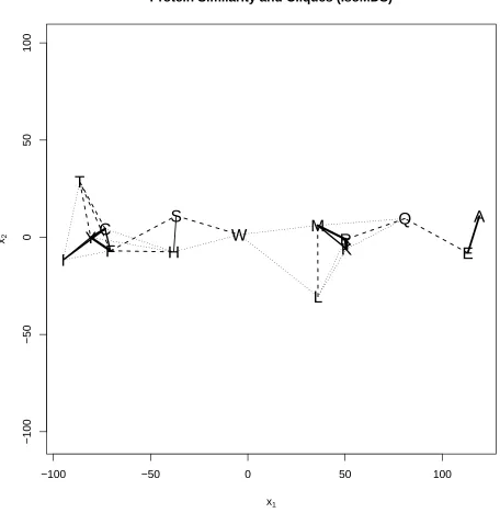
for use as additional information within a substitution matrix. Here we use the test statistics as a distance matrix to which multi-dimensional scaling [Mardia et al., 1979] can be applied. This

allows a graphical representation of which amino acids are more similar; the results are shown in Figure 1. It is interesting to note that the energy test cannot detect a difference between the distributions of Alanine (A) and Glutamic Acid (E) even though these have different side-chain

polarities and charges. We have tried, with some difficulty, to intepret the two axes in Figure 1. Although it is quite straightforward to describe the difference (or similarity) between any pair,

we have found it almost impossible to characterize the meaning of either dimension. We have observed that the amino acids towards the left of the plot tend to have more complex contours

in the region corresponding to theβ sheet. However, given that very few pairings are found to have similar distributions, it seems important not to pool together angles from different amino acids.

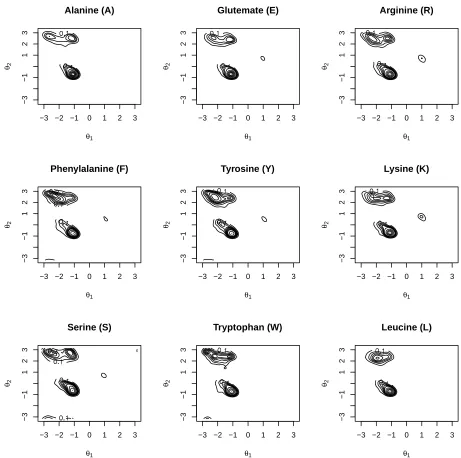
The kernel density estimate can be converted to probabilitycontours, orlevel setsas follows. Givenα, with (0≤α ≤1) define the setBα={(φ, ψ)|fˆ(φ, ψ) ≥t(α)}wheret(α) is a threshold

determined so that

Z Z

(φ,ψ)∈Bα

ˆ

f(φ, ψ)dφdψ= 1−α.

Aα−probability contour can then be drawn at the boundary ofBα. Some examples are shown in

Figure 2 (for similarities refer to Figure 1). Conversely, given a specific point (φ0, ψ0) a contour passing through this point will have a specific value ofα=α0, say which can be interpreted as a

measure of likelihood of occurrence at that location. It should be noted that these numbers are not probabilities but correspond to the usual p-value in a hypothesis test in the sense that, if the

null hypothesis is true, then the values will be uniformly distributed in [0,1]. These numbers can be used for validation as described in the next section.

5

Validation for new proteins

Given existing density estimates for each amino acid: ˆfA(φ, ψ),fˆC(φ, ψ), . . . these can be

con-verted (as above) to “probability functions”, say ˆPA(φ, ψ),PˆC(φ, ψ), . . .. Then for a “new” n-residue protein (which did not contribute training data to the density estimates) with{(Ai, φi, ψi), i=

1, . . . , n} we can compute a measure for the ith residue conditional on the amino acid type Ai,

−100 −50 0 50 100

−100

−50

0

50

100

Protein Similarity and Cliques (isoMDS)

x1

x2

A

C

E

F

H

I

K

L

M

Q

R

S

T

W

Y

Figure 1: Kruskal’s multidimensional scaling for the bootstrap test statistic to measure similarity

between the distributions of each pair of amino acids. Those connected by a continuous line have distributions which are not significantly different at 5%; dashed lines are similar at 1%, and dotted lines at 0.1%. Those amino acids which are not connected — and those which are not

Alanine (A)

θ1 θ2

−3 −2 −1 0 1 2 3

−3

−1

1

2

3

Glutemate (E)

θ1 θ2

−3 −2 −1 0 1 2 3

−3

−1

1

2

3

Arginine (R)

θ1 θ2

−3 −2 −1 0 1 2 3

−3

−1

1

2

3

Phenylalanine (F)

θ1 θ2

−3 −2 −1 0 1 2 3

−3

−1

1

2

3

Tyrosine (Y)

θ1 θ2

−3 −2 −1 0 1 2 3

−3

−1

1

2

3

Lysine (K)

θ1 θ2

−3 −2 −1 0 1 2 3

−3

−1

1

2

3

Serine (S)

θ1 θ2

−3 −2 −1 0 1 2 3

−3

−1

1

2

3

Tryptophan (W)

θ1 θ2

−3 −2 −1 0 1 2 3

−3

−1

1

2

3

Leucine (L)

θ1 θ2

−3 −2 −1 0 1 2 3

−3

−1

1

2

3

Figure 2: Contour (probability) plots of kernel density estimates for some example amino acids. Comparison with Figure 1 shows that the distributions of pairs (A,E), (R,K), (F,Y) are

mean. In practice, if there is a very small quantity, then the geometric mean, which is given by:

 



Y

jth amino acid type Y

{i:Ai=j}

ˆ

Pj(φi, ψi)

 

 1/n

(3)

is more likely to reveal this through a formal test. As is well-known, if the ˆP satisfy the null

hypothesis, then they will be uniformly distributed. Alternatively (or in addition), we can consider mini,jPˆj(φi, ψi), or the list p= (p1, . . . , p21) where

pj = min

{i:Ai=j}

ˆ

Pj(φi, ψi).

When a previously validated training dataset is used, a leave-one-out approach can be adopted

to provide a benchmark for the above quantities, by which future data can be compared. The proposed validation is formally intended to check both the labels (amino acids) and the angles.

Since the angles are derived from a set of 3-D ordinates, this would imply that the (relative) co-ordinates have been accurately determined. So, in the event that a protein “fails” the validation

test, this could be due to an incorrect amino acid label or inaccurate co-ordinates obtained from the X-ray technology. To distinguish between these two situations could be possible in some cases. However, in practice, the situation is a little more complicated as the sequence of

labels is assumed to be known, and often used (with prior knowledge) to suggest the co-ordinate structure. Note that this that this is a somewhat circular argument!

Using a cleaned up subset [Lovell et al., 2003] of the top 500 proteins from the Kinemage1 database, we can obtain a validation probability (using leave-one-protein-out cross-validation) for each protein. This dataset has 74,414 bivariate angles, with frequencies for each amino acid

given in Table 1.

A 7506 C 1299 D 4711

E 4132 F 3313 G 6865 H 1579 I 3772 K 3482

L 5968 M 1399 N 3083 P 1898 Q 2177 R 2621

S 4767 T 4639 V 5607 W 1153 Y 2838 Z 1605

Table 1: Frequencies of amino acids in the database of Lovell et al. [2003], with “Z” denoting pre-proline

The probabilities can be plotted (vs number of residues to improve clarity) and this plot,

together with a histogram, is shown in Figure 3. Given the nature of the data, it is not surprising that the smallest probability is about 0.158 (for protein 1tgsIH), which gives no cause for concern.

It is also reassuring that these probabilities do not seem to depend on size.

0 100 200 300 400 500 600 0.0 0.2 0.4 0.6 0.8 1.0

protein database: cross−validation probabilities

number of amino acids

fitted probability 119lH 153lH 16pkH 19hcAH 1a12AH 1a1yIH 1a28BH 1a2pAH 1a2zAH 1a3aDH _1a4iBH 1a62H 1a6mH 1a73AH 1a7sH 1a8dH 1a8eH 1a8iH 1aacH 1aayH 1abaH 1adsH 1agjAH 1ah7H 1ahoH 1aieH 1ajjH 1ajsAH 1ak0H 1akoH 1akrH 1amfH 1ammH 1ampH 1aohBH 1aopH 1aqbH 1aquAH 1aqzAH 1arbH 1aruH 1atgH 1atlACH 1atzAH 1auoAH 1avwBH 1axnH 1ay7BH 1aylH 1b0uH 1b0yH 1b16AH 1b3aAH 1b4kAH 1b4vH 1b5eAH 1b67AH 1b6aH 1b6gH 1b8oH 1b9wH 1babBH 1bb1AH 1bbhAH 1bbzEFH 1bd0AH 1bdmBH 1bdoH 1becH 1behBH 1benABH 1bf4AH 1bf6BH 1bfdH 1bfgH 1bg2H 1bg6H 1bgcH1bgfH 1bhpH 1bi5H 1bj7H 1bk0H 1bk7H 1bkbH 1bkjAH 1bkrH 1bm8H_1bpiH 1bqcH 1bqkH 1brtH 1bs0H 1bs9H 1bsmAH 1bteAH 1btkAH 1btyH 1bu7AH 1bu8H 1bueH 1bw9AH 1bx4H 1bx7H 1bxoH 1byiH 1byqH 1c02AH 1c1kH 1c1lH 1c24H 1c3dH 1c3pH 1c3wH 1c52H 1c5eAH 1c75H 1c90AH 1cb0H 1cc8H 1cczH 1cemH 1ceqH 1cexH 1cf9BH 1cgoH 1chdH 1cipH 1cjwH 1ckaH 1ckeH 1cl8H 1cmbAH 1cnvH 1cnzBH 1cpqH 1cruAH 1cs1AH 1ctfH 1ctjH 1cv8H 1cvlH 1cxcH 1cxqH 1cxyH 1cy5H 1cydAH 1cyoH 1czfAH 1czpAH 1d2nH 1d3vAH 1d7pH 1dbgH 1dbwBH 1dciAH 1dcsH 1df4H 1dfuPH 1dgfAH 1dhnH 1di6H 1difAH 1dinH 1dlfH 1dnlH 1dosAH 1dozH 1dp7PH 1dpsDH 1dptAH 1dqsAH 1dvjAH 1dxgAH 1ecoH 1edgH 1egwAH 1ejgH 1ek0H 1ek6AH 1elkAH 1ervH 1erxH 1es5H 1etnH 1euwH 1evhABH 1ezmH 1fdrH 1fdsH 1fkjH1flmBH 1flpH 1fmbH 1fnaH 1fncH 1ftrAH 1fusH 1fvkAH 1fxdH 1g3pH 1gaiH 1gcaH 1gceH 1gciH 1gd1OH 1gdjH 1gdoBFH 1gofH 1gpeAH 1gsoH 1guqAH 1gvpH 1h2rLH 1h2rSH 1hclH 1hfcH 1hfeSLH 1hkaH 1hmtH 1hpmH 1htrH 1hxnH 1iabH 1idoH 1iibAH 1isuAH 1ixhH 1jerH 1jetH 1jhgABH 1kapH 1koeH 1kp6H1kpfH 1kptAH 1kuhH 1kveABH 1lamH 1lbuH 1lclH 1lkkH 1lmb4H 1lstH 1lucBH 1m6pAH 1mbaH 1mctIH 1mdcH 1mfiAH 1mfmH 1mgtH 1mjhBH 1mlaH 1mmlH 1mofH 1molAH 1moqH 1mpgBH 1mrjH 1mroBH 1mroCH 1msiH 1mskH 1mugH 1munH 1narH 1nbcAH 1nddBH 1nfnH 1nifH 1nkdH 1nkrH 1nlsH 1notH 1noxH 1npkH 1nulBH 1nwpAH 1nzyBH 1oaaH 1oncH 1opdH 1orcH 1osaH 1pcfAH 1pdaH 1pdoH 1pefH 1penH 1pgsH 1phnAH 1plcH 1pmiH 1poaH 1psrAH 1ptfH 1pymAH 1qauH 1qb7H 1qcxH 1qczH 1qd1BH 1qddH 1qe3H 1qf9H 1qfmH 1qftAH 1qgiH 1qgqH 1qgwBDH 1qh4AH 1qh5AH 1qh8AH 1qh8BH 1qhfAH 1qhvH 1qipBH 1qj4H 1qjdH 1qk5AH 1qksAH 1ql0AH 1qlwAH 1qnfH 1qnjH 1qq4H 1qq5AH 1qqqH 1qreH 1qrrH 1qs1AH 1qsaH 1qsgGH 1qtsH 1qtwH 1qu9AH 1qupAH 1qusH 1ra9H 1rb9H 1rcfH 1rgeAH 1rhsH 1rieH 1rzlH 1sbpH 1sluH 1smdH 1smlH 1stnH 1svfABH 1svyH 1swuBH 1t1dH 1taxH 1tc1BH 1tcaH 1tenH 1tfeH 1thvH 1tifH 1tmlH 1toaAH 1tph1H 1ttbAH 1tudH 1tx4AH 1tyvH 1uaeH 1ubpH 1uchH 1ugiDH 1uroH 1ushH 1uteH1uxyH 1vcaAH 1vccH 1vfrAH 1vfyH 1vhhH 1vieH 1vjsH 1vnsH 1vsrH 1wabH 1wapBH 1whiH 1xikAH 1xjoH 1xnbH 1xwlH 1yacBH 1ygeH 1ytbAH 1yveIH 1zinH 256bAH 2a0bH 2actH 2acyH 2ahjCH 2ahjDH 2arcBH 2ayhH 2baaH 2bbkHH 2bbkLH 2bc2AH 2bopAH 2cbaH 2cbpH 2cpgAH 2cplH 2cppH 2ctcH 2cuaAH 2cypH 2dpmH 2driH 2endH 2engH 2erlH 2fdnH 2garH 2hbgH 2hftH 2hmzAH 2igdH 2ilkH 2kntH 2lisH 2mcmH 2mhrH 2msbAH 2myrH 2nacAH 2nlrH2porH 2pthH 2pvbH 2qwcH 2rn2H 2sakH 2sn3H 2spcAH 2tgiH 2tnfAH 2tpsAH 2trxAH 3btoAH 3chbDH 3chyH 3claH 3cyrH 3eipAH 3ezmH 3grsH 3htsBH 3nulH 3proCH 3pteH 3pviAH 3pypH 3sdhAH 3sebH 3silH 3stdAH 3vubH 451cH 4eugH 4lztH 4pgaAH 4xisH 5cytH 5hpgAH 5icbH 5nulH 5p21H 6celH 6gsvBH 7a3hH 7atjH 7fd1H 7odcH 7rsaH 8abpH 8rucAIH 9wgaAH 1fasH 1fltVH 1fltYH 1tgsIH 3ebxH 1edmBH 1tgxAH 1a92AH Frequency

0.0 0.2 0.4 0.6 0.8 1.0

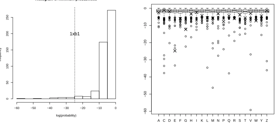
We now consider a hypothetical “new” protein1xb1— which is not in the training database

— using the proposed validation procedure, and compare the outcomes with Procheck [Laskowski

Histogram of minimum probabilities

log(probability)

frequency

−60 −50 −40 −30 −20 −10 0

0

50

100

150

200

250

1xb1

A C D E F G H I K L M N P Q R S T V W Y Z

−60

−50

−40

−30

−20

−10

0

Figure 4: Left: Histogram of log of the minimum tail probabilities for each of the Kinemage proteins, with minimum of the “test” protein 1xb1_{. Right: Boxplots of the log of the minimum}

tail probabilities by amino acid for the database, with extra points (×) corresponding to1xb1_.

et al., 1993], which is a commonly used tool for the validation of protein structures. (Procheck,

as well as MolProbity [Lovell et al., 2003] are used as part of a bigger validation tool provided by the Protein Data Bank.) The geometric mean for the angles is 0.28, which is well within a “normal” range of overall validation probabilities (Figure 3). The minimum ˆP is 1.7×10−11_,

which — at first sight — does look significant, and it is a particular residue (E) that Procheck associates with a “disallowed region”. However, if we consider a similar calculation for each of

the 500 Kinemage proteins, then this minimum ranks 14 — see Figure 4. Boxplots for each logpj

over the Kinemage database, with a comparison of the corresponding values for protein 1xb1

provides another visual check (Figure 4). More formal tests which compare the distribution of

the minimum amino acid tail probabilities of the Kinemage proteins with 1xb1 _{give p-values}

ranging around 0.1.

6

Discussion

The above probabilities all critically depend on the choice of smoothing parameter — λfor the von Mises kernel. In general, the smaller isλ(which corresponds to more smoothing), the larger is the validation probability, and the less sensitive is the test.

In principle, the above method could be used on any dataset. Ideally, one would liketraining

data which consists of a large database of independent bivariate observations which are known

of the λ’s which could be obtained by cross-validation (or a plug-in rule). Having stored the ˆ

P’s (on a reasonably fine grid on the torus) then formula (3) could be used to validate any new protein structure.

An alternative to cross-validation for selection of the λ’s is to consider an adaptive kernel bandwidth. Theoretical results — see, for example Terrell and Scott [1992] — suggest that using

a separate bandwidth for each observation, with a bandwidth that depends on density, will have better theoretical properties. This approach has been adopted by Lovell et al. [2003], although they have used an inefficient Cardioid kernel, and an adaptation that is not consistent with theory

which suggests that, for a von Mises kernel with concentration λ, the adaptive bandwith for observationishould satisfyλi ∝f(φi, ψi). However, limited simulation experiments suggest that

λi ∝f(φi, ψi)γ with γ ≈0.7 may work better for large datasets. Further work will investigate

this more closely, as well as examining which of the above proposed scores are more useful.

Acknowledgements

We are grateful to Simon Lovell for providing the filtered data from the “top 500” proteins. The

paper was improved after initial discussions with Andy Neuwald and Wally Gilks, both of whom also made helpful comments on an early draft.

References

Z. D. Bai, R. C. Rao, and L. C. Zhao. Kernel estimators of density function of directional data.

Journal of Multivariate Analysis, 27 (1988), 24–39.

R. Beran. Exponential models for directional data.The Annals of Statistics, 7 (1979), 1162–1178.

D. S. Berkholz, M. V. Shapovalov, R. L. Dunbrack, Jr. and P. A. Karplus. Conformation

dependence of backbone geometry in proteins. Structure, 17 (2009), 1316–1325.

W. Boomsma, K. V. Mardia, C. C. Taylor, J. Ferkinghoff-Borg, A. Krogh, and T. Hamelryck. A generative, probabilistic model of local protein structure. PNAS, 105 (2008), 8932–8937.

M. Di Marzio, A. Panzera and C.C. Taylor. Local polynomial regression for circular predictors.

Statistics and Probability Letters, 79 (2009), 2066–2075.

M. Di Marzio, A. Panzera and C.C. Taylor. Kernel density estimation on the torus. Journal of

Statistcal Planning and Inference, 141 (2011), 2156–2173.

S. R. Jammalamadaka and A. SenGupta. Topics in Circular Statistics. World Scientific, Singa-pore, 2001.

J. Klemel¨a. Estimation of densities and derivatives of densities with directional data. Journal

of Multivariate Analysis, 73 (2000), 18–40.

R. A. Laskowski, M. W. MacArthur, D. S. Moss, J. M. Thornton, PROCHECK - a program to check the stereochemical quality of protein structures. J. App. Cryst, 26 (1993), 283–291.

A. M. Lesk, ntroduction to protein science : architecture, function, and genomics. 2nd edition Oxford: Oxford University Press, 2010.

S.C. Lovell, I.W. Davis, W.B. Arendall III, P.I.W. de Bakker, J.M. Word, M.G. Prisant, J.S.

Richardson, and D.C. Richardson. Structure Validation by Cα Geometry: φ, ψ and Cβ Deviation. Proteins: Structure, Function and Genetics, 50 (2003), 437–450.

K. V. Mardia and P. E. Jupp. Directional Statistics. John Wiley, New York, NY, 1999.

K. V. Mardia, J. T. Kent and J. M. Bibby. Multivariate Analysis. London: Academic Press, 1979.

K.V. Mardia, C.C. Taylor, and G.K. Subramaniam. Protein bioinformatics and mixtures of

bivariate von mises distributions for angular data. Biometrics, 63 (2007), 505–512.

M. L. Rizzo Statistical Computing with R. Boca Raton: Chapman & Hall, 2007.

C. C. Taylor. Automatic bandwidth selection for circular density estimation. Computational

Statistics & Data Analysis, 52 (2008), 3493–3500.