An inverse problem of finding the time-dependent diffusion coefficient from an integral condition

This is a repository copy of An inverse problem of finding the time-dependent diffusion coefficient from an integral condition.

White Rose Research Online URL for this paper: http://eprints.whiterose.ac.uk/84756/

Version: Accepted Version

Article:

Hussein, M, Lesnic, D and Ismailov, MI (2016) An inverse problem of finding the

time-dependent diffusion coefficient from an integral condition. Mathematical Methods in the Applied Sciences, 39 (5). pp. 963-980. ISSN 0170-4214

https://doi.org/10.1002/mma.3482

[email protected] https://eprints.whiterose.ac.uk/ Reuse

Unless indicated otherwise, fulltext items are protected by copyright with all rights reserved. The copyright exception in section 29 of the Copyright, Designs and Patents Act 1988 allows the making of a single copy solely for the purpose of non-commercial research or private study within the limits of fair dealing. The publisher or other rights-holder may allow further reproduction and re-use of this version - refer to the White Rose Research Online record for this item. Where records identify the publisher as the copyright holder, users can verify any specific terms of use on the publisher’s website.

Takedown

If you consider content in White Rose Research Online to be in breach of UK law, please notify us by

An inverse problem of finding the time-dependent

diffusion coefficient from an integral condition

M.S. Hussein1,2_{, D. Lesnic}1 _{and M.I. Ismailov}3

1_{Department of Applied Mathematics, University of Leeds, Leeds LS2 9JT, UK}

2_{Department of Mathematics, College of Science, University of Baghdad, Baghdad, Iraq} 3_{Department of Mathematics, Gebze Institute of Technology, Gebze-Kocaeli 41400, Turkey}

E-mails: [email protected] (M.S. Hussein), [email protected] (D. Lesnic), [email protected] (M.I. Ismailov).

Abstract

We consider the inverse problem of determining the time-dependent diffusivity in the one-dimensional heat equation with periodic boundary conditions and nonlocal over-specified data. The problem is highly nonlinear and it serves as a mathematical model for the technological process of external guttering applied in cleaning admixtures from silicon chips. First, the well-posedness conditions for the existence, uniqueness and continuous dependence upon the data of the classical solution of the problem are established. Then, the problem is discretised using the finite-difference method and recast as a nonlinear least-squares minimization problem with a simple positivity lower bound on the unknown diffusivity. Numerically, this is effectively solved using the lsqnonlin routine from the MATLAB toolbox. In order to investigate the accuracy, stability and robustness of the numerical method, results for a few test examples are presented and discussed.

Keywords: Inverse problem; Thermal diffusivity; Integral condition.

1

Introduction

Parameter identification from over-specified data plays an important role in applied mathematics, physics and engineering. The problem of identifying the diffusivity was investigated by many researchers under various boundary and overdetermination condi-tions, [5–8, 14]. It is important to note that in [12], the time-dependent diffusion coef-ficient has been determined from different over-determination conditions in the case of self-adjoint auxiliary spectral problems.

2

Mathematical Formulation

In the rectangle QT = {(x, t)|0 < x < 1, 0 < t ≤ T} = (0,1)×(0, T], we consider the

inverse problem given by the heat equation

∂u

∂t(x, t) = k(t) ∂2_u

∂x2(x, t), (x, t)∈QT, (1)

with unknown concentration/temperatureu(x, t) and unknown time-dependent diffusivity k(t)>0, subject to the initial condition

u(x,0) =φ(x), 0_≤x_≤1, (2)

whereφ is a given function, the periodic and heat flux boundary conditions

u(0, t) = u(1, t), t_∈(0, T], (3)

ux(1, t) = 0, t∈(0, T], (4)

and the over-determination condition, [9, 10],

p(t)u(0, t) +

∫ 1

0

u(x, t)dx=E(t), t_∈[0, T], (5)

with p(t) = α+βk−γ_{(t), where α, β, γ > 0 are segregation coefficients. This problem}

arises in the mathematical modelling of the technological process of external guttering applied, for example, in cleaning admixtures from silicon chips, [10]. In this case, φ(x) is the distribution of admixture in the chip for x _∈(0,1) at the initial time t = 0, while u(x, t) is its distribution at time t. Condition (3) means that the admixtures in the left and right boundaries of the chip are the same. The adiabatic condition (4) means that the right boundaryx= 1 of the chip is perfectly insulated. Condition (5) means that part of the substance is concentrated (segregated) on the left side x= 0 of the chip, [9, 10].

When α=β = 0 then, the resulting inverse problem has been previously investigated in [5], and it is the purpose of this paper to investigate the non-trivial case when α and β are non-zero.

3

Mathematical Analysis

3.1

Existence and Uniqueness

The pair (k(t), u(x, t)) from the class C[0, T]_×(

C2,1_(Q

T)∩C1,0

( Q_T))

for which condi-tions (1)-(5) are satisfied andk(t)>0 on the interval [0, T],is called the classical solution of the inverse problem (1)-(5).

The analysis is similar to that of [4] for the identification of the time-dependent blood perfusion coefficient in the bio-heat equation. Consider the spectral problem

X′′(x) +λX(x) = 0, 0_≤x_≤1, (6)

X(0) =X(1), X′(1) = 0. (7)

It is easy to show that the problem (6) and (7) has the eigenvalues

λn = (2πn)2, n= 0,1,2, ...

and the system of eigenfunctions and associated functions

X0(x) = 2, X2n−1(x) = 4 cos(2πnx), X2n(x) = 4(1−x) sin(2πnx), n = 1,2, ... (8)

The system of functions Xn(x), n= 0,1,2, ... is a basis inL2[0,1], [3].

The adjoint problem to (6) and (7) has the form

Y′′(x) +λY(x) = 0, 0_≤x_≤1, (9)

Y(0) = 0, Y′(0) = Y′(1). (10)

Analogously to the problem (6) and (7), the system of eigenfunctions and associated functions of the problem (9) and (10) is given by

Y0(x) =x, Y2n−1(x) = xcos(2πnx), Y2n(x) = sin(2πnx), n= 1,2, .... (11)

It is easy to show that the systems (8) and (11) form a bi-orthonormal system on the interval [0,1], i.e.

(Xi, Yj) =

∫ 1

0

Xi(x)Yj(x)dx=δij,

whereδij is the Kronecker delta tensor.

The following lemmas are important for the mathematical analysis of the inverse problem.

Lemma 1. If ϕ(x) _∈ C3_{[0,1] satisfies the conditions ϕ(0) = ϕ(1), ϕ}′_{(1) = 0, ϕ}′′_{(0) =} ϕ′′_{(1) then the inequalities}

∞

∑

n=1

n2_|ϕ2n| ≤c1∥ϕ∥C3_[0,1],

∞

∑

n=1

n_|ϕ2n−1| ≤c2∥ϕ∥C3_[0,1], (12)

(c1 and c2 are constants)

hold, where ϕn= 1

∫

0

ϕ(x)Yn(x)dx.

Proof. Because ϕ(0) =ϕ(1), ϕ′′_{(0) =ϕ}′′_{(1), the equality}

ϕ2n = 1

∫

0

ϕ(x) sin (2πnx)dx =₋ 1 8π3_n3

1

∫

0

ϕ′′′_{(x) cos (2πnx)dx}

holds by three times integrating by parts. Analogously, by integrating by parts twice and using that ϕ(0) =ϕ(1), ϕ′_{(1) = 0 we obtain that}

ϕ2n−1 = 1

∫

0

ϕ(x)xcos (2πnx)dx=₋ 1 4π2_n2

1

∫

0

From the above, by using the Schwarz and Bessel inequalities we obtain

∞

∑

n=1

n2_|ϕ2n| ≤

1 8π3

[ _∞

∑

n=1

1 n2

]1₂    ∞ ∑ n=1   1 ∫ 0

ϕ′′′(x) cos (2πnx)dx   2   1 2

≤c1∥ϕ′′′∥L₂[0,1]≤c1∥ϕ∥C3_[0,1]

and

∞

∑

n=1

n_|ϕ2n−1| ≤

1 4π2

[ _∞

∑

n=1

1 n2

]1₂    ∞ ∑ n=1   1 ∫ 0

[xϕ′′(x) + 2ϕ′(x)] cos (2πnx)dx   2   1 2

≤ c₂2 ∥xϕ′′+ 2ϕ′_{∥L2[0,1] ≤}c2∥ϕ∥C3_[0,1]

for some constantsc1 and c2.

Lemma 2. If km(t) ∈ C[0, T] satisfies the condition 0 < a ≤ km(t), m = 1,2 then for ∀n_∈N _{and ∀t ∈[0, T] the inequality}

e−n

t ∫

0

k1(s)ds

−e−n

t ∫

0

k2(s)ds

≤ 1

ae∥k1 −k2∥C[0,T], (13)

holds.

Proof. For arbitrary fixedt _∈[0, T] and n_∈ N_{, by using the mean value theorem for the} functione−x _{we obtain that there exists θ betweenn}∫t

0

k1(s)ds and n t

∫

0

k2(s)ds such that

e−n

t ∫

0

k1(s)ds

−e−n

t ∫

0

k2(s)ds

=e−θ n t ∫ 0

k1(s)ds−n t

∫

0

k2(s)ds

.

By using thatxe−bx _≤ 1

be;x≥0, b=const. >0, we obtain that

ne−θ t ∫ 0

(k1(s)−k2(s))ds

≤e−natnt_∥k1−k2∥C[0,T]≤

1

ae∥k1 −k2∥C[0,T],

and this proves (13).

The main result of subsection 3.1 is in the following theorem.

Theorem 1. Let the functions φ(x)_∈C3_{[0,1], E(t)∈C[0, T] satisfy the conditions}

φ(0) =φ(1), φ′(1) = 0, φ′′(0) =φ′′(1), (14a)

φ2k ≥0, φ2k−1 ≤0, k = 1,2, ..., φ0+ 2φ1 <0, E(t)<2φ0,∀t∈[0, T], (14b)

where φn = 1

∫

0

φ(x)Yn(x)dx for n = 0,1,2,· · ·. Then, there exist positive numbers α0

and γ0 such that the inverse problem (1)-(5) with the parameters α < α0 , γ > γ0 has a

Proof. For arbitrary positivek(t)_∈C[0, T], using thatφ _∈C3_{[0,1] satisfies the conditions}

(14a), by applying the standard procedure of the Fourier series method we obtain the solution of the direct problem (1)-(4) in the following form:

u(x, t) =φ0X0(x) +

∞

∑

n=1

φ2ne

−(2πn)2∫t

0

k(s)ds

X2n(x)

+ ∞

∑

n=1

(φ2n−1−4πnφ2nt)e

−(2πn)2∫t

0

k(s)ds

X2n−1(x). (15)

The series in (15) and its x₋partial derivative are uniformly convergent in ¯QT since

their majorizing sums are absolutely convergent by Lemma 1. Therefore, their sums involved in expressingu(x, t) and ux(x, t) are continuous in ¯QT. Because the majorizing

sum ∑∞

n=1

n3_e−K(2πn)2_ε

(K =const. >0) is convergent, the t₋partial derivative and the xx₋second-order partial derivative series of (15) are uniformly convergent for t _≥ ε >0 (ε is an arbitrary positive number). Thus, we have u(x, t)_∈C2,1_(Q

T)∩C1,0

(¯ QT

)

which satisfies conditions (1)–(4) for arbitrary positivek(t)_∈C[0, T].

Applying the over-determination condition (5), we obtain

p(t) =̥_{[p(t)], (16)}

where

̥_{[p(t)] =}

2φ0 +_π2

∞

∑

n=1 1 nφ2ne

−(2πn)2∫t

0

k(s)ds

−E(t)

−2φ0+ 4

∞

∑

n=1

[4πnφ2nt−φ2n−1]e

−(2πn)2∫t

0

k(s)ds

,

k(t) =

[ β p(t)₋α

]1_γ

. (17)

Denote

α0 =

2φ0−Emax

−2φ0+ 4

∞

∑

n=1

(4πnφ2nT −φ2n−1)

, α1 =

2φ0+ 2_π

∞

∑

n=1 1

nφ2n−Emin −2φ0−4φ1

, (18)

where Emax = max

t∈[0,T]E(t), Emin = mint∈[0,T]E(t). Then, from (14b), (16) and (17) it follows

that

0< α0 ≤p(t)≤α1, t∈[0, T]. (19)

Under condition α0 > α, the inequalities

0< [

β α1−α

]_γ1

≤k(t)_≤

[ β α0−α

]1_γ

(20)

Let us denote

Cα0,α1[0, T] := {p(t)∈C[0, T]|α0 ≤p(t)≤α1,∀ t∈[0, T]}.

It is easy to verify that

̥_{:Cα0,α1[0, T]→Cα0,α1[0, T].}

Let us show that ̥ _{is a contraction mapping in Cα0,α1[0, T], for small α and large γ.} Indeed, _∀p1(t), p2(t)∈Cα0,α1[0, T] we have

̥_[p1(t)]−̥_{[p2(t)] =} 1

−2φ0+α1,2(t)

(

2φ0+α0,1(t)−E(t)

−2φ0+α1,1(t) (α1,2(t)−α1,1(t))−(α0,2(t)−α0,1(t))

)

, (21)

where

α0,m(t) =

2 π ∞ ∑ n=1 1 nφ2ne

−(2πn)2∫t

0

km(s)ds

,

α1,m(t) = 4

∞

∑

n=1

(4πnφ2nt−φ2n−1)e

−(2πn)2∫t

0

km(s)ds

,

km =

[ β pm(t)−α

]1_γ

, m= 1,2.

Lemma 2 and inequalities (20) imply

e−(2πn)

2∫t

0

k1(s)ds

−e−(2πn)

2∫t

0

k2(s)ds

≤ (α1−α)

1

γ

β1γe ∥

k1−k2∥C_[0,T].

Then, we obtain

|α0,2(t)−α0,1(t)| ≤

(α1−α)

1

γ

β1γe

( 2 π ∞ ∑ n=1 1 nφ2n

)

∥k1 −k2∥C[0,T],

|α1,2(t)−α1,1(t)| ≤

(α1−α)

1

γ

β1γe

(

16πT ∞

∑

n=1

nφ2n−4

∞

∑

n=1

φ2n−1

)

∥k1−k2∥C_[0,T].

From these inequalities and (21), we obtain

max

0≤t≤T|̥[p1(t)]−̥[p2(t)]| ≤

(α1−α)

1

γ

βγ1

δ_∥k1−k2∥C[0,T], (22)

where

δ = 2

πe

(8π2_{T α} 1+ 1)

∞

∑

n=1

nφ2n−2πα1

∞

∑

n=1

φ2n−1

−2φ0 −4φ1

. (23)

By using the mean value theorem and (20), it is easy to show that

|k1(t)−k2(t)| ≤

βγ1

γ(α0−α)1+

1

γ |

Thus, from (22) and (24) we obtain

∥̥_[p1]−̥_[p2]∥C [0,T]≤

δ (α0−α)

1 γ

(

α1−α

α0−α

)1/γ

∥p1−p2∥C_[0,T].

Let us fix a sufficiently large number γ0 >0 such that

K := δ

(α0−α)

1 γ0

(

α1−α

α0−α

)1/γ0

≤1. (25)

Thus, in the case γ > γ0, equation (16) has a unique solution k(t)∈ Cα0,α1[0, T], by the

Banach fixed point theorem.

We therefore obtain a unique positive function k(t), continuous on [0, T], which, to-gether with the solution of the problem (1)–(4) given by the Fourier series (15), form the unique solution of the inverse problem (1)–(5). This concludes the proof of the theo-rem.

3.2

Continuous Dependence Upon the Data

The following result on continuously dependence on the data of the solution of the inverse problem (1)–(5) holds.

Theorem 2. Consider the (input) data in the form of Φ = _{φ, E_} which satisfy the assumptions of Theorem 1 with

2φ0−Emax≥N1 >0, φ0+ 2φ1 ≤ −N2 <0 (26)

and let

∥φ_∥C3_[0,1]≤N3, ∥E∥C[0,T]≤N4 (27)

for some positive numbers N1, N2, N3 and N4. Then the solution (k(t), u(x, t)) of the

inverse problem (1)–(5) depends continuously upon the data for sufficiently small α and large γ.

Proof. Let Φ = _{φ, E_} and Φ = { φ, E}

be two sets of the data, which satisfy the conditions of Theorem 1. Let us denote _∥Φ_∥:=_∥φ_∥C3_[0,1]+∥E∥C_[0,T].

Let (k, u) and( k, u)

be solutions of the inverse problem (1)–(5) corresponding to the data Φ and Φ, respectively. According to (17),

p(t) =

2φ0+ 2_π

∞

∑

n=1 1 nφ2ne

−(2πn)2∫t

0

k(s)ds

−E(t)

−2φ0+ 4

∞

∑

n=1

[4πnφ2nt−φ2n−1]e

−(2πn)2

t ∫

0

k(s)ds

, k(t) =

[ β p(t)₋α

]1_γ ,

p(t) =

2 ¯φ0+ 2_π

∞

∑

n=1 1 nφ¯2ne

−(2πn)2∫t

0

¯ k(s)ds

−E¯(t)

−2 ¯φ0+ 4

∞

∑

n=1

[4πnφ¯2nt−φ¯2n−1]e

−(2πn)2∫t

0

¯ k(s)ds

, k¯(t) =

[ β ¯

p(t)₋α ]1_γ

First, let us estimate the differencep₋p¯. Using (12), (13) and (27), we obtain ∞ ∑ n=1 1 nφ2ne

−(2πn)2∫t

0

k(s)ds

≤ c_∥φ_∥

C3[0,1] ≤cN3,

∞ ∑ n=1

(4πnφ2nt−φ2n−1)e

−(2πn)2∫t

0

k(s)ds

≤ 4πc(1 +T)N3,

∞ ∑ n=1 1 nφ2ne

−(2πn)2∫t

0

k(s)ds −

∞

∑

n=1

1 nφ¯2ne

−(2πn)2∫t

0

¯ k(s)ds

≤ M1∥φ−φ∥

C3[0,1]+M2

k−k

C[0,T],

∞ ∑ n=1

(4πnφ2nt−φ2n−1)e

−(2πn)2∫t

0

k(s)ds −

∞

∑

n=1

(4πnφ¯2nt−φ¯2n−1)e

−(2πn)2∫t

0

¯ k(s)ds

≤ M3∥φ−φ∥

C3[0,1]+M4

k−k

C[0,T],

where Mk, k = 1,4 are some positive constants. By using these inequalities, simple

manipulations yield the estimate

|p(t)₋p(t)_{| ≤}

M5∥φ−φ∥

C3[0,1]+M6

k−k

C[0,T] +M7

E−E

C[0,T]

4N2 2

, (28)

whereMk, k= 5,7 are some constants that are determined by c1, c2 and Nk,k = 1,4.

It is known from (24) that, forα < α0,

k(t)−k¯(t)

≤

βγ1

γ(α0−α)1+

1

γ |

p(t)₋p¯(t)_|, (29)

with α0 ≥ _M2₈φ_∥0_φ−_∥Emax

C3[0,1] ≥

N1

M8N3, for some positive constant M8. If α is sufficiently small

such thatα < N1

M8N3, using (29) in (28) we obtain

(1₋M9)∥p−p∥_C[0,T] ≤M10

(

∥φ₋φ_∥

C3[0,1]+

E−E

C[0,T]

)

, (30)

for some positive constantsM10 and M9 := ₄M_N62 2

β1γ γ( N1

M₈N₃−α )1+ 1_γ.

The inequality M9 <1 holds for sufficiently largeγ. This means that p continuously

depends upon the data. Then, the equality k(t) = [_p(tβ_)−α]1/γ implies the continuous dependence of k upon the data. Similarly, we can prove that u, which is given in (15), depends continuously upon the data. This concludes the proof of the theorem.

4

Numerical Solution of Direct Problem

The discrete form of the direct problem is as follows. Take two positive integer M and N and let ∆x = 1/M and ∆t = T /N be step lengths in space and time directions, respectively. We subdivided the domain QT = (0,1)×(0, T) into M ×N subintervals

of equally step length. At the node (i, j) we denote ui,j = u(xi, tj), k(tj) = kj, where

xi = i∆x, tj = j∆t, for i = 0, M, j = 0, N. Considering the general partial differential

equation

ut=G(x, t, uxx), (31)

equation (31) subject to (2)–(4) can approximated as: ui,j+1−ui,j

∆t =

1

2(Gi,j+Gi,j+1), i= 1, M , j = 0,(N −1), (32)

ui,0 =φ(xi), i= 0, M , (33)

u0,j =uM,j, j = 0, N , (34)

uM+1,j =uM−1,j, j = 0, N , (35)

where

Gi,j =G

( xi, tj,

ui+1,j−2ui,j+ui−1,j

(∆x)2

)

, i= 1, M , j = 0,(N ₋1). (36)

For our problem, equation (1) can be discretised in the form of (32) as

−Aj+1ui−1,j+1+ (1 +Bj+1)ui,j+1−Aj+1ui+1,j+1 =

Ajui−1,j + (1−Bj)ui,j +Ajui+1,j, (37)

fori= 1, M,j = 0,(N ₋1), where

Aj =

(∆t)kj

2(∆x)2, Bj =

(∆t)kj

(∆x)2.

At each time step tj+1, for j = 0,(N −1), using the periodic boundary conditions (34),

the above difference equation can be reformulated as aM_×M system of linear equations of the form,

Duj+1 = Euj, (38)

where

uj+1 = (u1,j+1, u2,j+1, ..., uM,j+1)T,

D=



     

1 +Bj+1 −Aj+1 0 · · · 0 0 −Aj+1 −Aj+1 1 +Bj+1 −Aj+1 · · · 0 0 0

... ... ... . .. ... ... ...

0 0 0 _{· · · −}Aj+1 1 +Bj+1 −Aj+1

0 0 0 _{· · ·} 0 ₋2Aj+1 1 +Bj+1



     

M×M

,

and

E =



     

1₋Bj Aj 0 · · · 0 0 Aj

Aj 1−Bj Aj · · · 0 0 0

... ... ... ... ... ... ...

0 0 0 _{· · ·} Aj 1−Bj Aj

0 0 0 _{· · ·} 0 2Aj 1−Bj



     

M×M

4.1

Example

As an example, consider the direct problem (1)–(4) with T = 1 and

k(t) = 1 +t

2π2 , u(x,0) = φ(x) =−cos(2πx). (39)

The exact solution is given by

u(x, t) =₋cos(2πx)e−t2−2t. (40)

The required output (5) is

E(t) =p(t)u(0, t) +

∫ 1

0

u(x, t)dx=₋

(

α+β (

1 +t 2π2

)−γ)

e−t2−2t. (41)

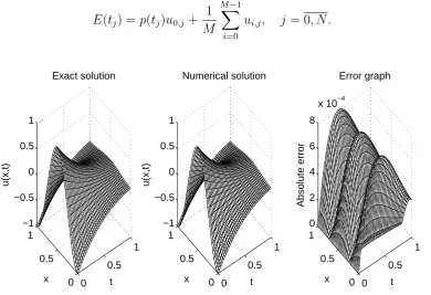
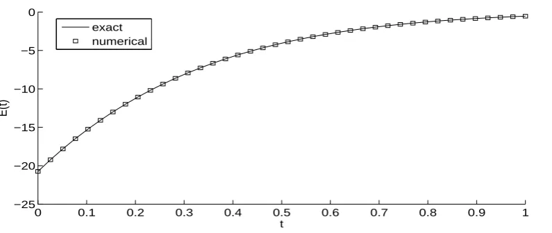
The numerical and exact solutions foru(x, t) at the interior points are shown in Figure 1 and also the absolute error between them is included. One can notice that an excellent agreement is obtained. Figure 2 shows the numerical solution in comparison with the exact one for E(t) for α = β =γ = 1. The numerical values for E have been calculated using equation (34) and the trapezoidal rule approximation to the integral in (41) to result in the formula

E(tj) =p(tj)u0,j+

1 M

M−1

∑

i=0

ui,j, j = 0, N . (42)

0 0.5

1

0 0.5 1 −1 −0.5 0 0.5 1

t Exact solution

x

u(x,t)

0 0.5

1

0 0.5 1 −1 −0.5 0 0.5 1

t Numerical solution

x

u(x,t)

0 0.5

1

0 0.5 1 0 2 4 6 8

x 10−4

t Error graph

x

Absolute error

0 0.1 0.2 0.3 0.4 0.5 0.6 0.7 0.8 0.9 1 −25

−20 −15 −10 −5 0

E(t)

t exact

numerical

Figure 2: Exact and numerical solutions for E(t) with α = β = γ = 1 for the direct problem obtained withM =N = 40.

5

Numerical Solution of Inverse Problem

We wish to obtain stable and accurate reconstructions of the time-dependent thermal conductivityk(t) and the temperatureu(x, t) satisfying the equations (1)–(5). We reduce the inverse problem to a nonlinear minimization of the least-squares objective function

F(k) :=

u(0, t)(α+βk−γ(t)) + ∫ 1

0

u(x, t)dx₋E(t)

2

L2_[0,T]. (43)

The discretised form of (43) is

F(k) =

N

∑

j=1

[

u(0, tj)(α+βkj−γ) +

1 M

M−1

∑

i=0

ui,j −E(tj)

]2

, (44)

where k = (kj)j=1,N, the values ui,j are computed from (38) and, for simplicity, we have

dropped the time-step multiplier T /N. It is worth mentioning that if the compatibility condition u(0,0) =φ(0) is satisfied then (5) applied at t= 0, yields

k(0) =

(

βφ(0) E(0)₋∫1

0 φ(x)dx−αφ(0)

)1/γ

. (45)

The minimization of the objective functional (44), subjected to the physical simple bound constraints k > 0 is accomplished using the MATLAB optimization toolbox routine lsqnonlin, which does not require supplying (by the user) the gradient of the objective function, [11]. Furthermore, within lsqnonlin we use the Trust-Region algorithm which is based on the interior-reflective Newton method, [2]. Each iteration involves a large linear system of equations whose solution, based on a preconditioned conjugate gradi-ent method, allows a regular and sufficigradi-ently smooth decrease of the objective functional (44), [1].

In the numerical computation, we take the parameters of the routine lsqnonlin as follows:

• Maximum number of iterations = 102_{×(number of variables).}

• Maximum number of objective function evaluations = 103_{×(number of variables).}

• Solution tolerance = 10−10_.

• Object function tolerance = 10−10_.

• Nonlinear constraint tolerance = 10−6_.

The inverse problem (1)–(5) is solved subject to both exact and noisy measurements (5). The noisy data is numerically simulated as

Eϵ(tj) =E(tj) +ϵj, j = 1, N , (46)

whereϵj are random variables generated from a Gaussian normal distribution with mean

zero and standard deviation σ given by

σ=ρ_× max

t∈[0,T]|E(t)|, (47)

where ρ represents the percentage of noise. We use the MATLAB function normrnd to generate the random variablesϵ= (ϵj)_j=1,N as follows:

ϵ=normrnd(0, σ, N). (48)

The total amount of noise ϵis given by

ϵ=ϵ

=

v u u t

N

∑

j=1

(Eϵ_(t

j)−E(tj))2. (49)

In the case of noisy data (46), we replace E(tj) by Eϵ(tj) in (44).

6

Numerical Results and Discussion

In this section, we present and discuss a few test examples in order to illustrate the accuracy, stability and robustness of the numerical scheme based on the FDM combined with the minimization of the least-squares functional (44), as described in Section 5.

6.1

Example 1

In this example, we consider the inverse problem (1)-(5) with T = 1 and the input data

u(x,0) = φ(x) =₋cos(2πx)

e , E(t) = − (

and α = β = γ = 1. One can easily check that E(t) _∈ C[0,1] and that C3_{[0,1] ∋ φ(x)}

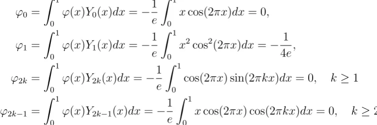
satisfies the conditions in (14a). Moreover, using (11) we have

φ0 =

∫ 1

0

φ(x)Y0(x)dx=−

1 e

∫ 1

0

xcos(2πx)dx= 0,

φ1 =

∫ 1

0

φ(x)Y1(x)dx=−

1 e

∫ 1

0

x2cos2(2πx)dx=₋ 1 4e,

φ2k =

∫ 1

0

φ(x)Y2k(x)dx=−

1 e

∫ 1

0

cos(2πx) sin(2πkx)dx= 0, k_≥1

φ2k−1 =

∫ 1

0

φ(x)Y2k−1(x)dx=−

1 e

∫ 1

0

xcos(2πx) cos(2πkx)dx= 0, k_≥2

and hence, one can easily check that the conditions in (14b) are also satisfied. We can also calculate from (18) and (23) that

α0 =

Emax

4φ1 ≃

74.45, α1 =

Emin

4φ1 ≃

79.95, δ = α1

e ≃29.41, (51)

where

Emax= max

t∈[0,1]E(t) = E(1) =−

1 + 8π2√₂

e√2 ≃ −27.38,

Emin = min

t∈[0,1]E(t) = E(1) =−

1 + 8π2

e ≃ −29.41.

Then the quantity K in equation (25) is given by K = 0.4004_{γ0 ×}(1.0749)1/γ0_{, and K ≤ 1}

if γ0 ≥ 0.5 for example. Anyway, our choice α = γ = 1 satisfies α < α0 = 74.45 and

γ > γ0 = 0.5 and hence according the Theorem 1 the solution of the inverse problem exits

and is unique. In fact, it can easily be checked by direct substitution that the analytical solution is given by

k(t) = 1

8π2√_{1 +t}, u(x, t) =−cos(2πx) exp(− √

1 +t). (52)

We take the initial guess for the unknown thermal diffusivityk(t) equal to the constant k(0) = 1/(8π2_{) which is known from expression (45).}

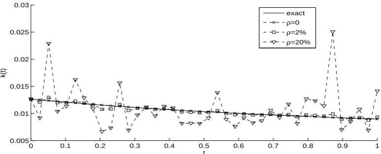
First, we attempt to retrieve the unknown diffusivity k(t) and the concentration/ temperature u(x, t) for exact input data, i.e. ρ = 0, as well as for ρ _{∈ {}2%,20%_} noisy data. The objective function (44) is plotted, as a function of the number of iterations, in Figure 3. From this figure, it can be seen that a very fast convergence is achieved in 4 to 8 iterations to reach a very low value of O(10−25_{). The associated numerically obtained}

0 1 2 3 4 5 6 7 8

10−30

10−25

10−20

10−15

10−10

10−5

100

105

Number of Iterations

Objective function

ρ=0 ρ=2% ρ=20%

Figure 3: Objective function (44), for Example 1 withρ_{∈ {}0,2%,20%_} noise.

0 0.1 0.2 0.3 0.4 0.5 0.6 0.7 0.8 0.9 1

0.005 0.01 0.015 0.02 0.025 0.03

t

k(t)

exact ρ=0 ρ=2% ρ=20%

0 0.5 1 0 0.5 1 −0.4 −0.2 0 0.2 0.4 t Exact solution x u(x,t) 0 0.5 1 0 0.5 1 −0.4 −0.2 0 0.2 0.4 t Numerical solution x u(x,t) 0 0.5 1 0 0.5 1 0 0.5 1

x 10−4

t Error graph x Absolute error (a) 0 0.5 1 0 0.5 1 −0.4 −0.2 0 0.2 0.4 t Exact solution x u(x,t) 0 0.5 1 0 0.5 1 −0.4 −0.2 0 0.2 0.4 t Numerical solution x u(x,t) 0 0.5 1 0 0.5 1 0 0.5 1

x 10−3

t Error graph x Absolute error (b) 0 0.5 1 0 0.5 1 −0.4 −0.2 0 0.2 0.4 t Exact solution x u(x,t) 0 0.5 1 0 0.5 1 −0.4 −0.2 0 0.2 0.4 t Numerical solution x u(x,t) 0 0.5 1 0 0.5 1 0 1 2 3 4

x 10−3

t Error graph

x

Absolute error

(c)

6.2

Example 2

Consider the inverse problem (1)-(5) withT = 1 and the input data

u(x,0) =φ(x) = ₋cos(2πx), E(t) = ₋

(

1 +

(

1 +t 2π2

)−1)

e−t2−2t, (53)

and α = β = γ = 1. As in Example 1, it is easy to check conditions (14a) and (14b) of Theorem 1 are satisfied. We also obtain that φk = 0 for all k ∈ N\ {1}, φ1 = −1/4,

Emin = E(0) = −(1 + 2π2) ≃ −20.73, Emax = E(1) = −(1 +π2)e−3 ≃ −0.516, and

α0 = Emax/(4φ1) = 0.516. As the condition 1 < α < α0 = 0.516 of Theorem 1 is not

satisfied we can not conclude the unique solvability of the inverse problem. However, the solution at least exists and is given by

k(t) = 1 +t

2π2 , u(x, t) = −cos(2πx) exp(−t 2

−2t). (54)

which can easily be verified by direct substitution.

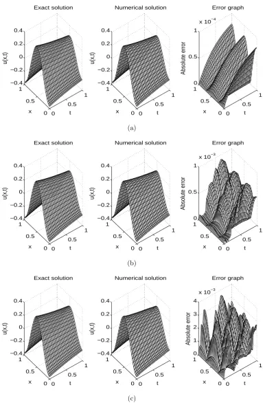
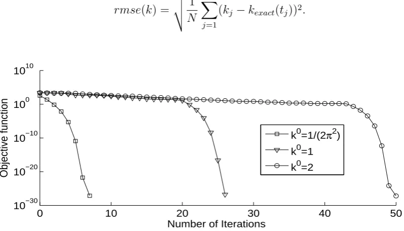
The FDM numerical solution of the direct problem associated to this example has already been presented and discussed in subsection 4.1. The uniqueness of solution (54) is not guaranteed from theory, but numerically we can at least investigate the obtained results from various initial guesses for the unknown diffusivity vector k which initiate the minimization of the objective function (44). This will also test the robustness of the iterative method with respect to the independence on the initial guess. This investigation is illustrated in Figures 6, 7 and Table 1 for exact data with various initial guesses

k0(t)_{∈ {}1/(2π2),1,2_}, t_∈[0,1]. (55)

Note that from (54) the initial guess k0(t) = 1/(2π2) corresponds to the value of k(0), which can be assumed to be known from (45). In Table 1, the root mean square error rmse value ofk is calculated as

rmse(k) =

v u u t

1 N

N

∑

j=1

(kj −kexact(tj))2. (56)

0 10 20 30 40 50

10−30 10−20 10−10 100 1010

Number of Iterations

Objective function

k0=1/(2π2)

k0=1 k0=2

0 0.1 0.2 0.3 0.4 0.5 0.6 0.7 0.8 0.9 11 0.05

0.06 0.07 0.08 0.09 0.1 0.11

t

k(t)

exact

k0=1/2π2

k0=1

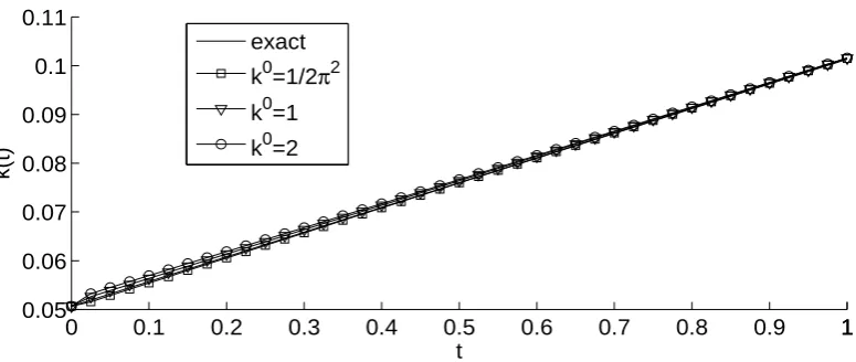
k0=2

Figure 7: Exact and numerical solutions for k(t), for Example 2 with no noise and various initial guesses (55).

Table 1: Number of iterations, number of function evaluations, value of the objective function (44) at final iteration,rmsevalue (56) and the computational time, for Example 2 with no noise and various initial guesses (55).

ρ= 0 k0 ₌ 1

2π2 k0 = 1 k0 = 2

No. of iterations 7 26 50

No. function evaluations 336 1134 2142

Value of objective function (44) at final iteration 7.3E-28 1.7E-27 6.2E-28

rmse(k) 1.6E-4 4.4E-4 7.6E-4

Computational time 31 sec 105 sec 198 sec

From Figure 6 and Table 1 it can be seen that, as expected, the farther the initial guess is the more iterations and larger computational time are required to achieve convergence. However, for all initial guesses (55) the objective function (44) converges to the same minimum low value ofO(10−28_{). This shows robustness with respect to the independence}

on the initial guess. Furthermore, from Figure 7 and Table 1 it can be seen that the agreement between the exact and the numerically obtained solutions with various initial guesses is very good being of O(10−4_{). There is also a slightly better accuracy for the}

closer initial guessk0 _{= 1/(2π}2_{) to the exact solution for k(t) from (54).}

In what follows, we take the initial guess for the unknown diffusivity k(t) equal to the constantk(0) = 1/(2π2_{) which is known from expression (45).}

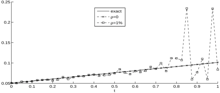
Figure 8 shows the objective function (44) forρ_{∈ {}0,1%_}as a function of the number of iterations. From this figure, it can be seen that the objective functional (44) decreases rapidly to a very low level of O(10−28_{) in about 7 to 8 iterations. The corresponding}

to add some regularization term λ_∥k_∥2

L2_[0,T] with λ >0 some regularization parameter to

the nonlinear least-squares function (43), but the stability of the numerical solution did not improve.

We also mention that for higher amounts of noise, such as ρ = 2%, the lsqnonlin minimization routine did not make significant progress after a large number of over 1000 iterations probably becoming trapped in a local minimum. One possible reason could be that the expressions fork(t) given by equations (52) and (54) yield a stronger nonlinearity ink−γ_{(t) in (43) for Example 2 than for Example 1.}

0 1 2 3 4 5 6 7 8

10−30

10−25

10−20

10−15

10−10

10−5

100

105

Number of Iterations

Objective function

ρ=0 ρ=1%

Figure 8: Objective function (44), for Example 2 withρ_{∈ {}0,1%_}noise.

0 0.1 0.2 0.3 0.4 0.5 0.6 0.7 0.8 0.9 1

0.05 0.1 0.15 0.2 0.25

t

k(t)

exact ρ=0 ρ=1%

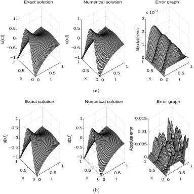
0 0.5 1 0 0.5 1 −1 −0.5 0 0.5 1 t Exact solution x u(x,t) 0 0.5 1 0 0.5 1 −1 −0.5 0 0.5 1 t Numerical solution x u(x,t) 0 0.5 1 0 0.5 1 0 1 2 3

x 10−3

t Error graph x Absolute error (a) 0 0.5 1 0 0.5 1 −1 −0.5 0 0.5 1 t Exact solution x u(x,t) 0 0.5 1 0 0.5 1 −1 −0.5 0 0.5 1 t Numerical solution x u(x,t) 0 0.5 1 0 0.5 1 0 0.005 0.01 0.015 t Error graph x Absolute error (b)

Figure 10: Exact and numerical solutions for u(x, t), for Example 2 with (a) no noise, and (b) ρ= 1% noise. The absolute error between them is also included.

6.3

Example 3

The previous examples possessed analytical solutions available for the pair (k(t), u(x, t)), as given by equations (52) and (54). In this subsection, we investigate an example for which an explicit analytical solution for u(x, t) is not available. We take the initial con-dition (2) given by

u(x,0) =φ(x) =

        

0, 0_≤x <1/4,

1

4 −x, 1/4< x≤1/2,

x₋ 3₄, 1/2< x <3/4, 0, 3/4< x_≤1.

(57)

given by

k(t) = 1

1 +t, t∈[0,1], (58)

in order to provide the data (5). This is performed numerically using FDM described in Section 4.

The numerical results for E(t) (with α = β = γ = 1) are shown in Figure 11, for various mesh sizes M = N _{∈ {}20,40,80_}. From this figure it can be seen that that numerical solution is convergent as the FDM mesh sizes decreases. Also, there is only a small difference between the numerical results obtained with various mesh sizes showing that the independence on the mesh has been achieved. Consequently, we take the results forE(t) simulated from solving the direct problem with M =N = 80 as our exact input data (5) in the inverse problem (1)–(5). In order to avoid committing an inverse crime, in the inverse problem the number of space intervals is taken asM = 70 (different than 80), whilst the number of time steps N is kept the same 80.

0 0.1 0.2 0.3 0.4 0.5 0.6 0.7 0.8 0.9 1

−0.3 −0.25 −0.2 −0.15 −0.1 −0.05

t

E(t)

(M,N)=(20,20) (M,N)=(40,40) (M,N)=(80,80)

Figure 11: Numerical solution forE(t), for the direct problem of Example 3 with various mesh sizes.

We take the initial guess k0 = 1, noting at the same time that since φ(0) = 0 and E(0) =₋1/16 equation (45) cannot be directly applied as it yields the non-determination 0/0 division.

Figure 12 shows the objective function evolution (44), as a function of the number of iterations for no noise in the input data (5). From this figure it can be seen that a fast convergence is achieved in 20 iterations to reach a very low value of O(10−12_{). The}

0 2 4 6 8 10 12 14 16 18 20

10−15

10−10

10−5

100

Number of Iterations

Objective function

Figure 12: Objective function (44), for Example 3 with no noise.

0 0.1 0.2 0.3 0.4 0.5 0.6 0.7 0.8 0.9 1

0.5 0.6 0.7 0.8 0.9 1

t

k(t)

exact numerical

0 5 10 15 20 25 30 35 40

10−15

10−10

10−5

100

Number of Iterations

Objective function

ε2

=7.05E−04

(a)

0 5 10 15 20 25 30 35 40

0 0.1 0.2 0.3 0.4

Number of iterations

rmse(k)

rmse=0.0587 rmse=0.0358 rmse=0.2110

(b)

Figure 14: (a) Objective function (44) with horizontal noise thresholdϵ2=7.05E-4, and (b) the rmse(k) values (56), for Example 3 with ρ= 1% noise.

Next we add ρ = 1% noise in the input data (5) numerically simulated as in (46). Figure 14(a) presents the objective function (44), as a function of the number of iterations together with the horizontal noise thresholdϵ2_{=7.05E-4 computed by (49). This threshold}

is useful when applying the discrepancy principle in order to stop the iteration process before the instability of solutions sets in. According to Figure 14(a) this criterion yields the iteration under iterdiscr. = 2. Figure 14(a) also shows that the objective function (44)

has converged after iterconv. = 38. Thermse(k) values (56) for unknown k(t) are plotted,

versus the number of iteration in Figure 14(b). Form this figure it can be remarked that the best retrieval occurs at iteropt. = 6. For more clarity, the results of Figure 14 are

summarised in Table 2 where the computational time is also included.

Finally, Figure 15 shows the exact solution (58) for k(t) in comparison with the nu-merical solutions obtained after the iterations given by stopping criteria of Table 2. From this figure it can be seen that if the iterative process is not stopped, after iterconv. = 38

we obtained a numerical approximation with rmse(k) = 0.2110 which moreover is not so accurate in the region t _∈ [0,0.2]. However, if we stop the iterative process after iterdiscr. = 2 iterations given by the discrepancy principle, which is graphically illustrated

associated numerically obtained results fork(t) plotted according to stopping criterion in Figure 15. From this figure it clear that the best retrieve for k(t) is the (--) lines which meets the minimumrmse value.

Table 2: The number of iterations, the rmse(k) values (56) and the computational time based on several stopping criteria, for Example 3 withp= 1% noise.

Criterion No. of iterations rmse(k) Computational time

to achieve convergence iterconv.= 38 0.2110 41 min

to achieve minimum rmse(k) iteropt.= 6 0.0358 8 min

discrepancy principle iterdiscr.= 2 0.0587 3 min

0 0.1 0.2 0.3 0.4 0.5 0.6 0.7 0.8 0.9 1

0 0.5 1 1.5

t

k(t)

Figure 15: Exact (—) and the numerical solutions for k(t) obtained after iterconv.=38 (- - -),

iteropt.=6 (--), and iterdiscr.=2 (-△-), for Example 3 with ρ= 1% noise.

7

Conclusions

An inverse nonlinear problem which requires identifying the time-dependent diffusivity with periodic boundary condition and non-local boundary measurement has been inves-tigated. The unique solvability and continuous dependence upon the input data have all been proved. Numerically, the resulting inverse problem has been reformulated as a nonlinear least-squares optimization problem which has been solved using the MATLAB toolbox routine lsqnonlin. Numerical results show that accurate, robust and reasonably stable solutions have been obtained. This problem seems rather stable and hence, in general, no regularization was found necessary to be employed. However, for more severe examples which violate the sufficient conditions under which the well-posedness of the inverse problem hold, as expected, some regularization needs to be applied. For example, in Subsection 6.3 for the minimization of the lsqnonlin routine used, the discrepancy principle has been applied in order to terminate the iterative process before instability sets in and this in turn has produced stable and accurate numerical solution.

References

[1] Baranger, T.N., Andrieux, S. and Rischette, R. (2014) Combained energy method and regularization to solve the Cauchy problem for the heat equation, Inverse Prob-lems in Science and Engineering, 22, 199-212.

[2] Conn, A., Gould, N. and Toint, P. (1987)Trust Region Methods, SIAM, Philadelphia. [3] Ionkin, N.I. (1977) Solution of a boundary-value problem in heat conduction with a

nonclassical boundary condition,Differential Equations, 13, 204-211.

[4] Ismailov, M.I. and Kanca, F. (2011) An inverse coefficient problem for a parabolic equation in the case of nonlocal boundary and overdetermination conditions, Math-ematical Methods in the Applied Sciences, 34, 692–702.

[5] Ismailov, M.I. and Kanca, F. (2012) The inverse problem of finding the time-dependent diffusion coefficient of the heat equation from integral overdetermination data, Inverse Problems in Science and Engineering, 20, 463–476.

[6] Ivanchov, M.I. (1994) Some inverse problems for the heat equation with nonlocal boundary conditions, Ukrainian Mathematical Journal,45, 1186-1192.

[7] Kanca, F. (2013) Inverse coefficient problem of the parabolic equation with periodic boundary and integral overdetermination conditions,Abstract and Applied Analysis, Vol. 2013, Article ID 659804, (7 pages).

[8] Lesnic, D., Yousefi, S.A. and Ivanchov, M. (2013) Determination of a time-dependent diffusivity form nonlocal conditions, Journal of Applied Mathematics and Computa-tion,41, 301-320.

[9] Muravei, L.A. and Petrov, V.M. (1987) Some problems of control of diffusion techo-logical process, In: Current Problems of Modelling and Control of System with Dis-tributed Parameters, Kiev, 42-43, (in Russian).

[10] Muravei, L.A. and Filinovskii, A.V. (1993) On a problem with nonlocal boundary condition for a parabolic equation,Math. USSR Sbornik, 74, 219-249.

[11] Mathworks R2012 Documentation Optimization Toolbox-Least Squares (Model Fit-ting) Algorithms, available from www.mathworks.com/help/toolbox/optim/ug /brnoybu.html.

[12] Namazov, G.K. (1984)Inverse Problems of the Theory of Equations of Mathematical Physics, Baku, Azerbaijan, (in Russian).

[13] Smith, G.D. (1985)Numerical Solution of Partial Differential Equations: Finite Dif-ference Methods, Clarendon Press, Oxford Applied Mathematics and Computing Sci-ence Series, Third Edition.