Signal Processing 86 (2006) 3496–3504
Fast communication
A nonlinear variational method for signal segmentation and
reconstruction using level set algorithm
Sasan Mahmoodi
a,, Bayan S. Sharif
baPsychology Department, School of Biology, Henry Wellcome Building Newcastle University, Newcastle upon Tyne NE2 4HH, UK bSchool of Electrical, Electronic and Computer Engineering, Merz Court, Newcastle University, Newcastle upon Tyne NE1 7RU, UK
Received 14 October 2005; received in revised form 19 June 2006; accepted 23 June 2006 Available online 18 July 2006
Abstract
A nonlinear functional is considered in this letter for segmentation and noise removal of piecewise continuous signals containing binary information contaminated with Gaussian noise. A discontinuity is defined as points in time scale that separates two signal segments with different amplitude spectra. Segmentation and noise removal of a piecewise continuous signal are obtained by deriving equations minimising the nonlinear functional. An algorithm based on the level set method is employed to implement the solutions minimising the functional. The proposed method is robust in noisy signals and can avoid local minima.
r2006 Elsevier B.V. All rights reserved.
Keywords:Level set method; Signal segmentation; Signal reconstruction; Nonlinear optimisation
1. Introduction
Variational methods in image and signal proces-sing have attracted considerable attention in recent years. Segmentation using variational methods was initially introduced by Kass et al.[1]and was further developed as the Geodesic Active Contours Model and the Level-Set Method [6]. On the other hand, Mumford et al.[12]introduced a nonlinear functional for segmentation and smoothing of images which was modelled as piecewise continuous functions that are surrounded by discontinuities represented by con-tours. This functional was further approximated for implementation using various approaches (e.g. see
[2–6,13–15]). However, it is well known that the optimal solution of nonlinear functionals considered in [12] is not unique [15] which results in the algorithms falling into local minima. A nonlinear functional similar to the one proposed in [12] was also considered by Mahmoodi et al.[8–11]for signal and image segmentation and noise reduction. In[9], the optimal solution to this functional for continuous and discrete signals is obtained and an algorithm based on this solution is proposed. A geometrical approach is employed in [8,10] to implement this functional for signal and image segmentation which leads to a robust algorithm in a noisy environment. Two terms are introduced in the functional consid-ered in[8–10]acting on the desired signal (or image): (1) fidelity which causes the desired signal to be as close as possible to the original noisy signal (2) smoothing the desired signal in proportion to a
www.elsevier.com/locate/sigpro
0165-1684/$ - see front matterr2006 Elsevier B.V. All rights reserved. doi:10.1016/j.sigpro.2006.06.012
Corresponding author. Tel.: +44 191 222 6246;
fax: +44 191 222 5622.
coefficient embedded in the functional. The compet-ing terms operate over a time segment where the original signal is considered continuous. It is demon-strated in [9] that points corresponding to disconti-nuities are minimisers of the functional. Therefore, the minimisation of such a functional leads to a unique solution representing the segmented and the smoothed signals. However, the smoothing term in
[8–10]introduces a low-pass filter whose bandwidth is related to the coefficient of the smoothing term. In this case, the desirable frequencies of a band pass input signal may be filtered by the smoothing term leading to the distortion of the smoothed signal. To overcome this problem, a modification to the functional considered in [8–10] is proposed in this letter to enable the algorithm to segment and reconstruct band pass signals containing high-frequency fluctuations. It is demonstrated that this method finds the global minimum by considering only the first variation of the functional. The level set method is employed to implement this func-tional and the results show that the proposed method is robust for signals with low SNRs. The basic principles are investigated in Section 2 whilst analysis and implementation based on the level set framework are considered in Section 3. Results are presented in Section 4 and finally conclusions are drawn in Section 5.
2. Basic principles
Discontinuities in a signal gðtÞ are defined as points in time scale separating segments over which the corresponding signals have different amplitude spectrums. If fiðtÞis a smooth continuous function of class Cn nX2 in the ith segment, a functional is
then considered as
Eðf;SÞ ¼X i
Z xi
xi1
½ðfiðxÞ gðxÞÞ2SiðxÞdx, (1)
whereSiðxÞis a windowed function representing the ith segment in whichgðxÞhas no discontinuities. In order to find the points corresponding to disconti-nuities, SiðxÞ has to be determined so that the ith
segment over which there is no discontinuity, is as long as possible. In this letter, we assume thatfiðxÞ
can be written as a linear combination of finite numbers of eigenfunctions of class Cn such as sin and cos functions, i.e.:
fiðxÞ ¼
X
m
ðAimcosðmoxÞ þBimsinðmoxÞÞ, (2)
where gðxÞ is considered periodic with a base frequency o¼2p=T and T is the entire time segment over which the whole signal is defined. Restriction imposed by (2) guarantees that fi is of class Cn over time segment i. A similar functional has been investigated in [4,8,9]; however, a major difference in the functional considered in this letter is that the continuity offifor theith time segment in functional (1) is imposed by the restriction presented in (2), whilst a smoothing term is explicitly introduced in the functional investigated in [4,8,9]. Let us now assume that gðxÞ is an even periodic function over the entire time length of the input signal, i.e., gðxÞ ¼gðxÞ. This assumption is used to reduce the number of calculated parameters by half without loss of generality. A half range expansion for fiðxÞ can then be employed [7], i.e.,
Bim¼0 and
Aim¼
Z xi
xi1
fiðxÞcosðmoxÞdt. (3)
Our minimisation problem is now reduced to determine the coefficients Aim and function SiðxÞ
minimising functional (1). In order to find the most optimised Aim, functions SiðxÞ are initially considered fixed. In the next section, equations leading to these coefficients are obtained in the level set framework. On the other hand, to find the most optimised SiðxÞ, variations of functional (1) should vanish by changing SiðxÞ.This requires that we consider the appropriate changes in fiðxÞ
as well.
3. Analysis and implementation
The proposed model by Chan et al.[4]in the level set formulation involves minimising functional (4):
Eðfi;fo;jÞ¼
Z T
0
ðfiðxÞ gðxÞÞ2þm dfi
dx
2
" #
HðjðxÞÞdx
þ
Z T
0
ðfoðxÞ gðxÞÞ2þm dfo
dx
2
" #
ð1HðjðxÞÞÞdx
þn
Z T
0
dHðjðxÞÞ dx
dx, ð4Þ
wherejis a Lipschitz function whose zero level set
with respect tofi,foand jare derived as:
md
2
fi
dx2 ¼fig for j40, (5)
md
2f
o
dx2 ¼fog for jo0, (6) qj
qt ¼ddðjÞ n
q qx
qj=qx jqj=qxj
ðgfiÞ2
þðgfoÞ2m dfi
dx
2
þm dfo
dx
2#
, ð7Þ
whereddðjÞis the regularised Dirac delta function.
Functional (4) is the one-dimensional Mumford– Shah functional in the level set framework. The Mumford–Shah functional and hence Chan–Vese model is based on the calculation of the first variation as discussed above. The solutions of the above differential equations are the segmented, and smoothed signals, i.e., discontinuities are the solutions of differential equation (7). Let us now assume a point atx¼xp corresponding tojðxpÞ ¼
0 which is not in a neighbourhood of any discontinuity. In this point, fiðxpÞ ¼foðxpÞ and
dfi=dxjx¼xp ¼dfo=dxjx¼xp, since we assume that gðxÞ is piecewise continuous of the class Cn, n42. It should also be noted that at such a point in the frontqjqx=jqjqxj ¼1 or1 and henceqðqjqx=jqjqxjÞ=qx¼0. Therefore, atx¼xp Eq. (7) vanishes. This analysis indicates that the point atx¼xpis a local minimum
of functional (4). In fact, the reason that the Chan–Vese model is trapped in local minima in piecewise continuous cases is due to an intrinsic feature in their model. This feature is introduced by treating Eq. (7) globally to detect discontinuities, whereas this equation should be treated as an equilibrium equation which is approximated in a neighbourhood of discontinuities [9]. The model proposed in [8,9] considers the second variation of a functional similar to (4) with respect to the fronts. It is proved in [9] that discontinuities are the minimisers of the functional and points away from any discontinuities that are saddle points of the functional and therefore should be discarded. In this short letter, however, we demonstrate that it is also possible to avoid local minima by considering only the first variation in the cases where a signal is composed of a finite number of frequency components so that each time segment contains a number of complete cycles of each frequency. The advantage of using only the first
variation is that less numerical complexity is introduced, since the second variation calculations are not required.
Let us now consider functional (1) in the level set framework:
EðAi;Ao;jÞ
¼a
Z T
0
X
m
AimcosðmoxÞ gðxÞ
!2 2
4
3
5HðjðxÞÞdx
þb
Z T
0
X
m
AomcosðmoxÞ gðxÞ
!2
2 4
3 5
ð1HðjðxÞÞÞdx, ð8Þ
where j is a Lipschitz function whose front (jðxÞ ¼0) represents discontinuities. Hð:Þ in (8) represents the regularised Heaviside function and thereforeHðjÞand 1HðjÞforjðxÞ40 represent intervals over which signals are characterised with different amplitude spectrums. Functional (8) in the level set formulation is equivalent to functional (1) with the restriction indicated in (2). Optimal values for the coefficients in (2) are obtained by vanishing the derivative ofEwith respect toAipforpX0 (i.e.,
qE=qAip¼0Þ.
Z T
0
cosðpoxÞgðxÞHðjðxÞÞdx
¼
Z T
0 X
m
AimcosðpoxÞcosðmoxÞHðjðxÞÞdx. ð9Þ
A similar linear system to (9) can be derived forAom.
Functional (8) is also minimised with respect to the signed distance function j. This therefore leads to the following Euler–Lagrange equation:
qj
qt ¼ddðjÞ a g
X
m
AimcosðmoxÞ
!2 2
4
þb gX
m
AomcosðmoxÞ
!23
5, ð10Þ
whereddðjÞis the regularised Dirac delta function.
Differential equation (10) coupled with a linear system such as (9) for different time intervals should be solved iteratively.jand hence discontinuities are iteratively evolved to converge to the desired solution. Upon convergence, the discontinuities corresponding to jðxÞ ¼0 represent the segmented signal (segmentation) and Fourier coefficients Aim
reduction). For the simplicity of the analysis in this short letter, we assume that signal gðxÞconsists of only one frequency component with two different amplitudes. As demonstrated in the next section, the numerical simulations indicate that the proposed algorithm in this letter can be applied to signals with
any number of frequency components. However, a mathematical argument for signals containing multiple frequencies is not presented here. It is noted that the proposed method in this letter is only applicable to signals with time segments containing a number of complete cycles of a frequency or a set
[image:4.544.35.497.168.647.2](a) (b) (c)
(a)
(b)
[image:5.544.109.440.61.631.2](c)
of frequencies. A signal with a single carrier frequency is usually considered in communications. In this case, Eq. (10) is written as
qj
qt ¼ddðjÞ½aðgAicosðo0xÞÞ
2
þbðgAocosðo0xÞÞ2. ð11Þ
CoefficientsAiandAo are then calculated as
Ai¼
RT
0 cosðo0xÞgðxÞHðjÞdx RT
0 cos2ðo0xÞHðjÞdx
, (12)
Ao¼
RT
0 cosðo0xÞgðxÞð1HðjÞÞdx RT
0 cos2ðo0xÞð1HðjÞÞdx
. (13)
(a)
(b)
[image:6.544.106.443.69.527.2](c)
In a signal with only one discontinuity, we assume a pointPatx¼xpwhich is not in a neighbourhood
of a discontinuity atx¼xdso thatxd4xp. It is also
assumed that point P is in the time domain over which the sinusoidal signal has amplitude Gi.
The other part of signal is characterised with a sinusoidal signal with amplitudeGoaGi. From the above equations,Ai andAo are calculated as
Ai¼
Rxp
0 cosRðo0xÞðGicosðo0xÞÞdx
xp
0 cos2ðo0xÞdx
¼Gi (14)
or
Ao ¼Goþ ðGiGoÞ I0
I0þI1
, (16)
where I0¼Rxxpdcos2ðo0xÞdx and
I1¼RxTdcos2ðo0xÞdx. Therefore, Eq. (11) can be
written as
qj
qt ¼ddðjÞ b
ðGiGoÞ2I20
ðI0þI1Þ2
cos2ðo0xÞ
. (17)
The right-hand side of Eq. (17) corresponds to a force driving the front (j¼0) towards the discontinuity. This driving force exists as long as the front does not correspond to the discontinuity. However, in a discontinuity xp¼xd hence I0¼0 implying Ai¼ GiandAo¼Go. Therefore, Eq. (11) representing the
first variation vanishes only in a discontinuity. In the presence of noise, Eq. (11), still vanishes, although the front might be slightly shifted with respect to the discontinuity in the original signal. This analysis demonstrates that a point corresponding to disconti-nuity is a minimiser of functional (8). This property prevents the algorithm from falling into a local minimum. The above analysis applies to a signal with any number of discontinuities, i.e., if a segment of the input signal is in the ‘wrong’ part ofj(j40), it produces a negative term in Eq. (10) and hence creates two new discontinuity points (or zero cross-ings in j). This argument is also true for the case where the ‘wrong’ part of j corresponds to jo0. This fact is due to the well-known property of the level set formulation based on which the algorithm can be adjusted to the topology of the
input data. It is also noted that the minimisation of functional (8) leads to the segmentation and recon-struction of signals with binary information where the original signal consists of a time sequence of two types of signals with different amplitude spectra. The described evolution procedure occurs only if the signed distance function is correctly initialised. This is because the right side in iterative equation (10) should be comparable to the initial signed distance function to be able to change the level set function for the evolution of the
algorithm. Throughout this letter, the signed distance functionjðxÞis initialised as
jðxÞ ¼1
4 2 T x T 2 , (18)
where T is the total length of the input signal. The above signed distance function initially corresponds to only two discontinuities. However during the evolu-tion of the algorithm, the number of discontinuities changes to match the number of discontinuities in the input signalgðxÞ. In this letteraandbin Eq. (10) are set to 1. These coefficients can, however, be set to a value corresponding to the maximum absolute ampli-tude of the input signal. For signals with low absolute amplitude, higher values for these coefficients should be chosen to allow Eq. (10) to evolve. The algorithm proposed in this letter, is summarised in pseudo-code below. The signed distance function j is firstly initialised by using Eq. (18). Differential equation (10) is then solved to updatejðxÞand hence evolve the fronts representing discontinuities. In each iteration, a one-dimensional Gaussian filter is applied tojðxÞto regularise the differential equation (10), which im-proves the robustness of our algorithm.
1. Initialisej0 for n¼0
Loop:
2. Compute Aim and Aom
3. Solve differential equation forjto obtain jnþ1
4. Apply Gaussian low pass filter tojnþ1
If convergence is not reached,
Thenn¼nþ1and goto step 2;
Otherwiseend theLoopand goto step 5 5. Reconstruct the signal using Aimand Aom Ao ¼
Rxd
xp cosðo0xÞðGicosðo0xÞÞdxþ
RT
xdcosðo0xÞðGocosðo0xÞÞdx
RT xpcos
2ðo 0xÞdx
¼ GiI0þGoI1 I0þI1
4. Results
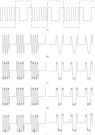
A synthetic signal with eight discontinuities is shown inFig. 1(first row). The level set functionj, segmented and reconstructed signals in four different iterations of the algorithm are depicted in the second to the fifth row of Fig. 1. The dashed curves in all figures show the different segments of the signals. In this example, the bandwidth of the Gaussian
low-pass filter is set top=3. Fig.2compares the proposed method for segmentation and reconstruction of signals with a method in which the optimised functional contains an explicit smoothing term (see e.g.[4]). The original signal is shown inFig. 2a. The proposed method in this letter is applied to the original signal and the segmented and reconstructed signals are presented inFig. 2b. The segmented and reconstructed signals using the traditional methods in
(a)
(b)
(c)
(d)
[image:8.544.106.435.188.654.2](e)
the literature (e.g.[4]) are depicted inFig. 2c. As can be seen from this figure, the Chan–Vese algorithm converges to a local minimum, i.e., segmented and reconstructed signals do not correspond to the original signal. In this example,m¼10 and n¼10. If m increases, the reconstructed signal becomes smoother and hence more distorted, whereas if the value of m is reduced, the algorithm over-segments the signal. This problem becomes more severe when noise is added to the original signal. In the third example, a synthetic noiseless signal depicted in
Fig. 3a is contaminated with a Gaussian noise to produce the noisy signal shown in Fig. 3b with SNR¼1. The segmented and reconstructed signals are demonstrated in Fig. 3c. A signal containing several discontinuities with two different frequencies is shown inFig. 4. In this example, we aim to show that the proposed method can segment and recon-struct the signal based on discontinuities in frequency rather than those in the signal itself. Fig. 4a shows the original signal. As shown in this figure, the signal is composed of two square waves with different frequencies. The segmentation is achieved based on the first harmonic. Having segmented the signal, more harmonics can be employed for reconstruction. The segmented and reconstructed signals using only the first frequency harmonic is shown inFig. 4b, and using three, five and 30 harmonics in Figs. 4c–e, respectively. It is interesting to note that in this example discontinuous signals are reconstructed by using a set of continuous eigenfunctions. The fluctuations and oscillations in the reconstructed signals in Fig. 4e are due to Gibbs phenomenon. Segmentation and reconstruction of signals of the type shown inFig. 4a are not possible by minimising any functional containing an explicit smoothing term of the desired reconstructed signal, since the desired signal contains discontinuities.
5. Conclusion
A new method is proposed in this letter to find the global minimum in a minimisation problem leading to signal segmentation and noise reduction of a given noisy signal. A functional is considered for this purpose and continuity of each segment of the signal is implicitly imposed in comparison with the previous functionals in which continuity was explicitly presented. Numerical comparison has been made between the proposed method and the traditional method. The level set method is em-ployed to implement this functional. The algorithm
presented in this letter converges very easily, is robust in the presence of noise and can reconstruct desired signals containing discontinuities.
Acknowledgements
Authors would like to thank the anonymous reviewers for their constructive and interesting comments.
References
[1] M. Kass, A. Witkin, D. Terzopoulos, Snakes: active contour models, Internat. J. Comput. Vis. 1 (1988) 321–331. [2] T.F. Chan, B.Y. Sandberg, L.A. Vese, Active contours
without edges for vector-valued images, J. Vis. Commun. Image Representation 11 (2000) 130–141.
[3] T.F. Chan, L.A. Vese, Active contours without edges, IEEE Trans. Image Process. 10 (2) (2001) 266–277.
[4] T.F. Chan, L.A. Vese, Level set algorithm for minimising the Mumford–Shah functional in image processing, in: Proceed-ings IEEE Workshop on Variational and Level Set Methods in Computer Vision, 2001, pp. 161–168.
[5] M. Hintermuller, W. Ring, An inexact-CG-type active contour approach for the minimization of the Mumford– Shah functional, J. Math. Imaging Vis. 20 (2004) 19–42. [6] G. Aubert, P. Kornprobst, Mathematical Problems in Image
Processing: Partial Differential Equations and Calculus of Variations, Springer, New York, 2002.
[7] E. Kreyszig, Advanced Engineering Mathematics, Wiley, New York, 1999.
[8] S. Mahmoodi, B.S. Sharif, Signal segmentation and denois-ing algorithm based on energy optimisation, Signal Proces-sing 85 (9) (2005) 1845–1851.
[9] S. Mahmoodi, B.S. Sharif, Noise reduction, smoothing, and time interval segmentation of noisy signals using an energy optimisation method, IEE Proc. Vis. Image Signal Process. 153 (2) (2006) 101–108.
[10] S. Mahmoodi, B.S. Sharif, Nonlinear optimisation method for image segmentation and noise reduction using geome-trical intrinsic properties, Image Vis. Comput. 24 (2006) 202–209.
[11] S. Mahmoodi, B.S. Sharif, Unsupervised texture segmenta-tion using a nonlinear energy optimisasegmenta-tion method, J. Electron. Imaging 15 (3) (2006) in press.
[12] D. Mumford, J. Shah, Optimal approximations by piecewise smooth functions and associated variational problems, Comm. Pure Appl. Math. 42 (4) (1989) 577–688.
[13] A. Tsai, A. Yezzi, A.S. Willsky, Curve evolution implemen-tation of the Mumford–Shah functional for image segmen-tation, denoising, interpolation and magnification, IEEE Trans. Image Process. 10 (8) (2001) 1169–1186.
[14] L.A. Vese, Multiphase object detection and image segmenta-tion, in: S. Osher, N. Paragios (Eds.), Geometrical Level Set Methods in Imaging, Vision, and Graphics, Springer, Berlin, 2003, pp. 175–194.
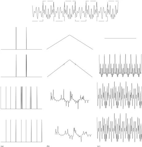
![Fig. 2. Original noiseless signal (a) segmented and reconstructed signal using the proposed method in this letter (b) segmented andreconstructed signals using the methods of differential equations considered previously in literature with m ¼ 10 and n ¼ 10 (e.g., [4]) (c).](https://thumb-us.123doks.com/thumbv2/123dok_us/8503139.348077/5.544.109.440.61.631/noiseless-reconstructed-andreconstructed-differential-equations-considered-previously-literature.webp)