TECHNICAL DOCUMENTATION OF I3E MODEL VERSION 2 ESRI SURVEY AND STATISTICAL REPORT SERIES NUMBER 77 September 2019

EV

IDENCE FOR POLIC

Y

TECHNICAL DOCUMENTATION OF I3E MODEL

VERSION 2

KELLY

DE BRUIN

AND

AYKUT MERT YAKUT

ESRI

Technical Documentation of I3E Model, Version 2

Kelly de Bruin

Aykut Mert Yakut

September 2019

ESRI SURVEY AND STATISTICAL REPORT SERIES

NUMBER 77

Available to download from www.esri.ie

©_{The Economic and Social Research Institute}

Whitaker Square, Sir John Rogerson’s Quay, Dublin 2

ISBN 978-0-7070-0501-0

DOI https://doi.org/10.26504/sustat77

This Open Access work is licensed under a Creative Commons Attribution 4.0 International License (https://

ABOUT THE ESRI

The mission of the Economic and Social Research Institute is to advance evidence-based policymaking

that supports economic sustainability and social progress in Ireland. ESRI researchers apply the highest

standards of academic excellence to challenges facing policymakers, focusing on 12 areas of critical importance to 21st Century Ireland.

The Institute was founded in 1960 by a group of senior civil servants led by Dr T. K. Whitaker, who

identified the need for independent and in-depth research analysis to provide a robust evidence base for policymaking in Ireland.

Since then, the Institute has remained committed to independent research and its work is free of any expressed ideology or political position. The Institute publishes all research reaching the appropriate

academic standard, irrespective of its findings or who funds the research.

The quality of its research output is guaranteed by a rigorous peer review process. ESRI researchers are experts in their fields and are committed to producing work that meets the highest academic standards

and practices.

The work of the Institute is disseminated widely in books, journal articles and reports. ESRI

publica-tions are available to download, free of charge, from its website. Additionally, ESRI staff communicate

research findings at regular conferences and seminars.

The ESRI is a company limited by guarantee, answerable to its members and governed by a Council,

com-prising 14 members who represent a cross-section of ESRI members from academia, civil services, state

agencies, businesses and civil society. The Institute receives an annual grant-in-aid from the Department of Public Expenditure and Reform to support the scientific and public interest elements of the Institute’s

activities; the grant accounted for an average of 30 per cent of the Institute’s income over the lifetime

of the last Research Strategy. The remaining funding comes from research programmes supported by government departments and agencies, public bodies and competitive research programmes.

THE AUTHORS

Kelly de Bruin is a Research Officer at the Economic and Social Research Institute (ESRI). Aykut Mert

Yakut is a Postdoctoral Research Fellow at the Economic and Social Research Institute (ESRI).

ACKNOWLEDGEMENTS

The research carried out in this report was funded by the Department of Communications, Climate Action

and Environment (DCCAE) and is part of an ongoing modelling project.

EXECUTIVE SUMMARY

This paper provides a technical description of the Ireland Environment, Energy and Economy (I3E)

model. The I3E model is an intertemporal computable general equilibrium model with multiple firms, one representative household group, multiple commodities, government, enterprises, and rest of the world

accounts. It describes the Irish economy in sectoral detail. This model includes a detailed description of

1

Introduction

Climate change and the associated challenges are at the forefront of current policy debates. For example,

all countries have committed to the Paris Climate agreement (with the exception of the US). In line with this, climate policy is becoming increasingly important domestically, as Ireland is obliged to decrease

its emissions under the EU Commission’s Climate and Energy Package. Ireland is required to deliver a

20% reduction in non-ETS greenhouse gas emissions by 2020 relative to 2005 levels, increasing to 30% in 2030. Designing appropriate energy policies is imperative to ensure a smooth and least-cost transition

to a low-carbon economy. Furthermore, a better understanding of the implications of such a transition

is necessary, especially on a sectoral level, to identify those sectors most hit by climate policies. In this sense data-based economic models can be very useful to advise policy, giving insights into the

real-world effects of different policy measures. Such models can investigate the economic costs and sectoral

implications of reaching the EU goals and which specific climate policies (e.g., carbon tax, energy tax or quotas) can be implemented to reach these goals, accounting for the economic behaviour of producers

and consumers.

To analyse the impacts of energy-related policies on the Irish economy, a model with sectoral details and various energy inputs and technologies is needed. With this objective in mind, the Ireland

Environ-ment, Energy and Economy model (I3E model) is developed. This model focusses on the relationship

between the economy, energy inputs and environmental impacts in the form of greenhouse gas (GHG) emissions. The I3E model is an intertemporal computable general equilibrium (CGE) model with

mul-tiple firms, one representative household group (RHG), mulmul-tiple commodities, government, enterprises,

and rest of the world accounts.

This paper serves as a reference document concerning the technical details of the I3E model. In what

follows, the model structure and equations will be presented

This document is structured as follows. In the next section, the sets, which represent the dimensions of the model, will be defined and clarified. Section3 presents the equations dictating the behaviour

of each agent in turn. Section4 discusses the description of commodities in the model. In Section5, the quantities are discussed and in Section 6, the prices. The energy part of the model is discussed

in Section7. Section 8describes how economic growth is incorporated in I3E. Section 9explains the

savings–investment behaviour, and Section10gives the equilibrium conditions. The lists of activities and commodities can be found in AppendixA, the list of endogenous variables is presented in AppendixB,

and finally, AppendixCprovides the list of exogenous variables and parameters. This document describes

2

Sets

The variables and parameters used within the model are defined over various sets, which are collections

of different variables or parameters with common characteristics. Each set has a unique definition and contains elements that meet the defined criteria. The set logic is used to define equations over appropriate

sets and allows us to exclude variables in the solution process. Each set and potential subsets are described

in what follows.

• Activities

All activities are assigned to the set a. This is the broadest set for domestic production activities. Along with several dimensions, activities are assigned to several subsets as follows

– Firm behaviour

An Activity determines its level of investment, i.e. investment by destination, by dividend maximisation as explained in Section3.2.1. This procedure is based on Tobin’sq, which is defined as the market value of a firm’s capital stock divided by the replacement cost of it; in

other words, the marginal value of capital. If a firm’s total investment expenditure is high,

the market value and the replacement cost of its capital stock are of a similar magnitude and Tobin’sqapproaches unity. If it is less than unity, the firm should not invest anymore. In the calibration process, some of the activities’ Tobin’sqvalues are calibrated as less than unity, and these activities are considered non-dividend maximisers. See Section3.2.1for details. Dividend maximising firms are assigned to the subset dma and non-dividend maximising firms tondma.

– Production across commodities

Activities are allowed to produce multiple products, and the quantity of production is

deter-mined by revenue maximisation as explained in Section3.2.4. However, some activities either produce a single commodity or their production of a single commodity exceeds 95% of their

total production. For these activities, total output is a Leontief aggregate of the commodity (if

the activity is the unique producer) or commodities (if the production of a commodity exceeds the cut-off point). Otherwise, the activity’s output is a constant elasticity of transformation

(CET) aggregate of commodities that are produced by the activity in the base-year.

Activities for which the output is defined by CET function are assigned to the subset aceta and activities where the output is defined by a Leontief function are assigned to the subset

aleoa.

– Energy demand

The sets a1a−a4a are created to distinguish activities concerning the composition of their energy demands by setting different elasticity of substitution values. The nested structures of

• Commodities

All commodities are assigned to the setcwhich includes the following subsets:

– Origin

The setcpccontains commodities produced by domestic producers and sold in the domestic market. This set is defined over commodities for which the cells of activity rows and

com-modity columns on the Social Accounting Matrix (SAM) are positive. The setcpnc covers

non-domestically produced commodities

– Exports

The set cec is defined over export commodities, i.e. commodities for which the cells of commodity rows and the rest of the world columns on the SAM are positive. The setcenc is the complementary set that coversnon-exported commodities.

– Imports

The set cmc contains import commodities, i.e. commodities for which the cells of the rest of the world rows and commodity columns on the SAM are positive. The set cmnc covers non-imported commodities.

– Homogeneity

As explained in Section3.2.4, activities are allowed to produce multiple products; however, there are a few commodities produced by a single activity, for instance, public administration.

In this case, the commodity is homogeneous and assigned to the setchc. This set covers com-modities for which the elasticity of substitution for the domestically produced commodity,

σ_c,tqxcs, is zero. The set chnc is the complementary set that coversnon-homogeneous

com-modities, i.e. commodities that are produced by at least two distinct activities and σc,tqxcs is positive.

– Composite goods

The model includes detailed nested structures of private composite consumption and

pro-duction. The primary objective of creating such detailed nested structures is to reflect the compositions of households’ and activities’ demands for energy commodities as accurately

as possible. In this sense, the way the nested structure is defined determines the

substitutabil-ity between inputs to production and between goods for consumption. If goods are nested together, this represents higher substitutability between these goods compared to others. A

Leontief relationship assumes no substitutability, whereas a constant elasticity of substitution (CES) relationship assumes a substitution possibility. The values of the elasticity of

substitu-tion parameter, σ, for different elasticity relations are chosen in order to reflect the low and

high substitution possibilities among the commodities based on expert judgement.

• Margins

• Factors of production

The set f contains factors of production. In this version, it has two elements, Labour and Capital.

– Capital

One type of capital (physical capital) is defined in the model.

– Labour

The set lhas three elements: low skilled labour (LSL), medium skilled labour (MSL), and high skilled labour (HSL). The sectoral composition of employment by skill is retrieved from

the Labour Force Survey (LFS). For each type of households hh, the composition of wage income by skill is retrieved from the Survey on Income and Living Conditions (SILC).

• Households

The set hh is the broadest set for households. In this model version, there are ten RHGs (five groups in urban areas and five groups in rural areas). These RHGs have been generated based on

disposable income by using the Household Budget Survey (HBS). The survey has also been used to derive the composition of consumption expenditures across commodities and the distribution of

household disposable income across different income items.

• Time

The settcomprises the horizon of the model and takes values between 2014 and 2054. In conven-tional CGE modelling, parameters do not have a time index. However, several parameters of the I3E model have a time index to generate a flexible model which allows dynamic simulations to be

run. For instance, if the government wants to implement a policy change in 2020, the value(s) of

3

Agents

This section discusses the behaviour of each agent in the model in turn. The agents in the I3E model

consist of households, activities, commodities, enterprises, and government,

3.1 Households

In this version, it is assumed that there is one RHG that solves the following intertemporal utility

max-imisation problem where the utility function is in the form of Constant Relative Risk Aversion (CRRA):

max

CChh,t

∞

∑

t=1

1+grwt 1+ρhh

t

(CChh,t)1−θhh 1−θhh

s.t

SAV_hh,t +PCC_hh,tCC_hh,t ≤W INC_hh,t +CINC_hh,t +T R_hh,t +

PEN_hh,t+ NFI_hh,t ERt + RCIhh,t RCHHt

(1)

wheregrwt is the economic growth rate in the periodt,ρhhis time preference rate,θhh is intertemporal elasticity of substitution,W INChh,t,CINChh,t,T Rhh,t,PENhh,t, andNFIhh,t are net-of-tax wage income, net-of-tax capital income (distributed dividends of enterprises), transfers from the government, pension income from the government, and net factor incomes from abroad (fixed in real terms), respectively,

ERt is exchange rate,SAVhh,tis savings,CChh,t is household-specific composite consumption andPCChh,t is its price. The termRCIhh,t is the carbon tax recycling income from the government and RCHHt is a parameter (which is equal to zero in the calibration process) that allows for running an experiment in

which the government recycles the carbon tax collection to households. The RHS of the budget constraint represents household disposable income,INChh,t. The components of disposable income are as follows.1

W INChh,t =

_∑

γ_l,hh,twage

_∑

Wl,tW FDISTa,l,t LDa,l,t (1−wtaxl,t) (2)

whereγ_l,hh,twageis the share of householdhhin the total wage income of labour typel, andwtaxl,t is the wage income tax rate of labour typel.

CINChh,t = γhh,tcincDISDIVt (3)

whereγ_hh,tcinc is the share of householdhh in the total dividend (capital / asset) income. In this set-up, household savings are determined endogenously by

SAVhh,t = INChh,t − PCChh,tCChh,t (4)

1 _{For the sake of space saving, explanations of variables and parameters will be given in the relevant subsections. You can see}

Householdhhchooses the level of composite consumption to maximise the present discounted value of intertemporal utility. The first-order condition (FOC) of this problem, eq. (5), is the well-known consumption Euler equation and solves for the sequence of composite consumption wherert is interest rate.

CChh,t+1

CChh,t =

(1+grwt)

1+rt+1

1+ρhh

PCChh,t

PCChh,t+1

_θ1 hh

(5)

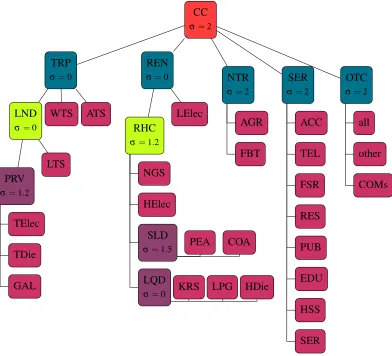
In the second stage, householdhhdisaggregates her composite consumption across commodities by max-imising her intratemporal utility. The nested structure of household composite consumption is depicted by Figure1.

CC

σ=2

TRP

σ=0

LND

σ=0

PRV

σ=1.2

TElec TDie GAL LTS WTS ATS REN

σ=0

RHC

σ=1.2

NGS

HElec

SLD

σ=1.5 PEA COA

LQD

σ=0 KRS LPG HDie

LElec

NTR

σ=2

AGR

FBT

SER

σ=2

ACC TEL FSR RES PUB EDU HSS SER OTC

σ=2

all

other

COMs

Figure 1: Nested Structure of Consumption

Several composite commodities are included in the consumption nest; these are either constant elas-ticity of substitution (CES) or Leontief aggregates of directly observed commodities and/or other

com-posite commodities. For the CES aggregates of the comcom-posite commodities, the values of elasticity of

Household composite consumption,CC, is assumed to be a CES aggregate of composite commodities of Transportation (T RP), Residential Energy (REN), Nourishment (NT R), Services (SER), and other commodities (OTC). As described above, this reflects that different services goods are easier to substitute with each other than, for example substituting services goods with nourishment goods. The logic here

is that consumers are more likely to substitute food products with, e.g., agricultural products if prices of food products increase than to increase their consumption of services as food prices increase.

The composite commodityT RPis a Leontief aggregate of land, air, and water transportation com-modities where land transportation (LND) is also a Leontief aggregate of public and private transportation commodities. The choice of a Leontief relationship here is warranted by the low level of substitutability

between transport types; a consumer will not substitute their daily car commute with air or water transport due to increases in petrol prices. It should be noted that the original land transportation commodity (LT S

with NACE Code 49) covers the public transportation demand of households. In I3E, we assign a share of

household demand energy commodities including gasoline, diesel, and electricity for private transporta-tion purposes. We refer to private transportatransporta-tion energy use as the composite commodityLND, which is assumed to be a Leontief aggregate of that energy commodities.2 TheRENis disaggregated into lighting electricity and residential heating which is further disaggregated into natural gas supply, solid fuel, heat-ing electricity, and liquid fuel. Moreover, solid (liquid) fuel is a CES (Leontief) aggregate of peat and

coal (kerosene, liquid petroleum gas, and diesel for heating purposes). The total electricity consumption

of households, the commodityELC, is known from the SAM, and it is disaggregated into electricity de-mand by transportation, lighting, and heating purposes by using the data provided bySEAI(2013, Table

19). Similarly, total private consumption of diesel is disaggregated into diesel demand for transportation

and heating by using the energy balances. The composite commodityNT Ris a CES aggregate of the commodities agriculture and food, beverage, and tobacco while the composite commoditySERis a CES aggregate of several service commodities. The composite commodityOTC is a CES aggregate of all remaining commodities that are demanded by households.

The compositions of electricity and diesel demands across their sub-components are assumed to be

identical across households as there are no data available to make a further distinction. Moreover, the

values of elasticity of substitution shown in Figure1are also assumed to be the same across households.

3.2 Activities

3.2.1 Investment by Destination

The term “investment by destination” refers to investment expenditures of firms / sectors. In the model

we distinguish between dividend maximisers and non-dividend maximisers; we discuss each in turn. In a fully intertemporal setting, the investment decision can be endogenised via a dividend maximisation

2 _{According to the energy balances, the private consumption of liquid petroleum gas is devoted both to private transportation}

problem where a firm maximises the present discounted value of its dividend stream,DIVdm,t (i.e. the present value of firm,Vdm,t) by choosing the level of physical investment,PSIdm,t, and levels of factors of production (i.e. capital,K_dm,t, and composite labour,CLD_dm,t).

max

PSIdm,t,Kdm,t,CLDdm,t

V_dm,t =

∞

∑

t=1

1+grwt 1+rt

t

DIV_dm,t s.t (6)

Kdm,t+1(1 + grwt) = (1−δdm,t)Kdm,t +PSIdm,t (7) whereδdm,t is the depreciation rate. Activity-specific capital stock (Kdm,t) evolves according to capital accumulation function, eq. (7). The Lagrange multiplier of this maximisation problem,qdm,t, which is constrained by capital accumulation function is the well-known Tobin’s q3, i.e. the marginal value of capital:

DIV_dm,t = (1−cor ptaxt)W Kdm,t Kdm,t − INVdm,t (8)

INVdm,t = PPSIt PSIdm,t+ PVAdm,t ADJdm,t (9)

ADJdm,t=φdm,t

PSI_dm,t2 Kdm,t

(10)

whereW K_dm,t is the price of capital andPPSIt is the price of the investment. The sectoral dividend is equal to net-of-corporate tax sectoral profit minus total investment expenditures,INVdm,t, which includes the cost of new investment equipment and the adjustment cost. Adjustment cost is an increasing and convex function of investment; for a given level of sectoral capital stock, the cost of installing new

capital equipment will be greater. Adjustment cost,ADJdm,t, is measured by the price of the value added,

PVAdm,t, because it is assumed that installation of new capital requires the resources of the firm, which leads to interruption of the production process and thus losses of output.

The FOCs of this dividend maximisation problem w.r.t. the levels of physical investment and capital

stock, respectively, are as follows.

qdm,t = PPSIt + 2PVAdm,t

ADJdm,t

PSIdm,t

(11)

q_dm,t (1+rt) (1 + grwt) = qdm,t+1(1−δdm,t) + PVAdm,t+1

ADJdm,t+1

Kdm,t+1

+ (1−cor ptaxt)W Kdm,t+1

(12)

For non-dividend maximisers, the investment (by destination) expenditure in periodtof an activity is a fixed fraction of its total profits in periodtas follows, whereγ_ndm,tinvdesis a fixed parameter.

INV_ndm,t = γ_ndm,tinvdesW Kndm,t Kndm,t (13)

The level of investment expenditures determines the level of physical investment demand of a firm (PSIndm,t) which, in turn, determines the level of sectoral capital stock (Kndm,t).

INVndm,t = PPSIt PSIndm,t (14)

Kndm,t+1(1 + grwt) = (1−δndm,t)Kndm,t +PSIndm,t (15) The depreciation rate of these firms is arbitrarily set to be equal to 0.05.

For all firms, either in the subset of dmorndm, the real value added,VAa,t, is a CES aggregate of sectoral capital stock and sectoral composite labour

VAa,t =λ_a,tva[γ_a,tcvaK−ρ va a,t

a,t + (1−γa,tcva)CLD −ρava,t a,t ]

− 1

ρ_ava,t ₍₁₆₎

whereCLDa,t is composite labour demand,γa,tcvais the share parameter of capital in real value added,λa,tva is the shift parameter, andρ_a,tvais the exponent parameter and obeysσ_a,tva=1/(1+ρ_a,tva).

The value added is equal to the sum of the payments to the factors of production

PVAa,tVAa,t = W Ka,t Ka,t +CWa,tCLDa,t (17)

whereCWa,t is price of sectoral composite labour input.

As the sectoral capital stocks evolve by following the law of motion for capital (7and15), the FOC of the cost minimisation problem yields the optimal level of composite labour demand

CLDa,t = "

PVAa,t γ_a,tcva

CWa,t (λa,tva)ρ va a,t

#σava,t

VAa,t (18)

Since the model comprises there types of labours, it is assumed that an activity chooses a sector-specific composite labour input which is a CES aggregate of different types of labour. Each activity

solves a cost minimisation problem to find the optimal combination of types of labours that minimises

the cost of labour.

min

LDa,l,t

CWa,tCLDa,t =

_∑

LD_a,l,tWe_l,tW FDIST_a,l,t s.t (19)

CLDa,t = "

∑

l

γ_a,l,tcld (BXt LDa,l,t)−ρ cld a,t

#− 1 ρacld,t

whereLDa,l,t is labour demand of the activity,Wel,t is the wage per effective labour,W FDISTa,l,t is the ratio of factor payments to labourlfrom activityato the wage rate of labourl,BXt is the level of labour productivity,γ_a,l,tcld is the share of labour type l in composite labour input of activity a, and ρ_a,tcld is an exponent parameter. We need the termW FDISTa,l,t since the wage rate is determined by equilibrium conditions in the labour market for each type of labour, i.e. the model solves for three wage rates. However, since productivity of each type of labour is different, payments to labour cannot be the same

across sectors. The term captures the distance between average and sectoral payments to labour.

In the case of labour-augmented technological growth, activities choose the level of “efficient labour”,

i.e. the multiplication of the labour demand and the level of productivity. Given the technological change,

the wage per effective labour,Wel,t, is constant while the wage per labour,Wl,t – the wage received by labour – grows at the rate of technological change. For the given level of labour supply, labour is paid

more in every period due to increases in its productivity. Hence, the following relation holds.

Wl,t = Wel,tBXt

The optimal level of labour demand is determined by

BXt LDa,l,t = "

CWa,t γ_a,l,tcld BXt

Wl,tW FDISTa,l,t #σacld,t

CLDa,t (21)

3.2.2 Production

The total value of production, the LHS of eq. (22), is equal to payments to factors of production, i.e.

value-added, production taxes paid to the government, the total cost of intermediate inputs, and the cost

of the Emissions Trading System (ETS).

PXa,t QXa,t = PVAa,tVAa,t+ PRODTAX Sa,t + PCINa,tCCINa,t +CET Sa,t (22)

whereQXa,t is an activity’s total production andCCINais composite intermediate input demand; PXa,t andPCINa,tare their prices, respectively.

The production of activities in the model is represented by a nested structure as shown in Figure2. To

reflect the differences in energy demand compositions, activities are assigned to three distinct groups at two different layers of the nested production structure. The elasticity of substitution parameter,σ, takes

the value of 0 for activities which have a quite strict composition of energy demand. On the other hand,

its value is either 1.1 or 1.3 for activities whose composition of the energy demand is not dominated by a specific energy commodity.

inter-QX

σ=2

VA

σ=2

K CLD

σ=2

LSL MSL HSL

BEN

σ1=0,

σ2=1.1,

σ3=1.3

FUE

σ1=0,

σ2=1.1,

σ3=1.3

GAL KRS FUO LPG DIE

EElec BH

σ1=0,

σ2=1.1,

σ3=1.3

PEA COA CRO NGS BElec

OTI

σ=2

All

other

inputs

Figure 2: Nested Structure of Production, except Electricity Production

mediate inputs except the energy commodities. The composite labour is a CES aggregate of three types of

labour. For all activities, except the electricity production, the commodityBENis assumed to be an aggre-gate of energy electricity (EElec), fuel (FU E) and business heating (BH). The composite commodityBH

is an aggregate of liquid and solid fuels including coal, peat, crude oil, natural gas supply, and business

electricity for heating purposes. On the other hand, the composite commodityFU E is an aggregate of gasoline, kerosene, fuel oil, liquid petroleum gas, and diesel. The electricity demand of activities, except the electricity production, is disaggregated across demands for energy purposes and heating/combustion

purposes.4 The nested structure of production of all activities except electricity production is depicted by Figure2.

The electricity production activity has a unique production technology and energy demand

compo-sition. The activity’s business energy, BEN, is assumed to be a CES aggregate of electricity, natural gas, and other energy (OT E) which is a CES aggregate of all remaining energy commodities, as shown in Figure3. The value ofσ is 1.1 for the commodity ofBEN while it is 1.3 for theOT E because the electricity production has more flexibility to substitute between liquid and solid fuels than natural gas and

electricity’s itself.

4 _{At this stage, the disaggregation is done by arbitrarily assuming that 40% (60%) of the total sectoral electricity is used for}

QX

σ=2

VA

σ=2

K CLD

σ=2

LSL MSL HSL

BEN

σ=1.1

NGS ELC OTE

σ=1.3

PEA COA CRO GAL KRS FUO LPG DIE

OTI

σ=2

All

other

inputs

Figure 3: Nested Structure of Electricity Production

3.2.3 Emissions Trading System

The ETS is the European Union’s (EU) key tool to reduce industrial emissions. In the current phase of the

system, Phase-III that covers the period of 2013–2020, each installation (i.e. a production unit) receives an amount of free allowances (EU-ETS,2018). If the installation’s total emissions exceed its free allowances,

the installation will need to purchase additional allowances5at the ETS price determined in the EU-wide ETS market. If the installation emits less than its free allowances, it can sell its unused allowances to other installations at the EU-ETS price. In other words, the system generates a cost (revenue) for those

installations which emit more (less) than their allowances. An installation may generate more revenue

from the ETS system by reducing its emissions as it invests more on cleaner production technologies. Therefore, the last term on the RHS of eq. (22) is a cost (revenue) item if it is positive (negative).

The coverage of sectoral emissions by the ETS is 100% for the energy production sectors; energy

production installations do not receive any free allowances and need to purchase allowances to cover all their emissions. Petroleum refining, mineral, and aviation sectors’ emissions are also fully covered by the

ETS, but installations operating in these industries receive some free allowances. On the contrary, land transportation (road or railway), agriculture, waste, and residential sectors are exempted from the ETS.

For the other sectors, the ETS coverage varies based on the average size of production units regarding the

combustion capacity, production capacity, etc. (EPA,2018).

In the I3E model, economic activities directly internalise the cost of ETS in their cost minimisation

problems. As an example, the optimal level of an intermediate input in the composite commodity of

business heating (BH)is

INTc,a,t = "

PCINBH,a,t γ_c,a,tbh

PQDc,t + ET SADJc,a,t #σabh,t

CCINBH,a,t (23)

whereINTc,a,t in intermediate input demand on commodityc by activity a,CCINBH,a,t is intermediate demand on the composite commodityBHby activityaandPCINBH,a,t is its price, andγc,a,tbh andσa,tbhare share and exponent parameters of the CES function, respectively.6 The denominator in the parentheses is the total unit cost of a commoditycfor activityawherePQDc,t is purchaser price of commoditycand

ET SADJc,a,tis the ETS adjuster such that

ET SADJc,a,t = PET St ET StoEa,t (1−AtoTa,t)carconc (24)

wherePET St is the EU-ETS price of a per ton emission allowance,ET StoEa,t is the ratio of ETS emis-sions to total emisemis-sions of activitya,AtoT_a,t is the ratio of ETS allowance to ETS emissions of activity

a, andcarconc is the carbon content of commodity cwhich is calibrated by dividing total emission of commoditycby its total consumption for the year of 2014.7

The EU-ETS price is an exogenous variable since it is determined in the EU-wide allowance market,

which is not explicitly incorporated in the I3E model. The ratio of ETS emissions to total emissions of

an activity is a parameter (i.e. its value for each activity is calibrated by using the realised values of total and ETS emissions in 2014), and its value is assumed to be constant through time. However, the ratio of

ETS allowance to ETS emissions of an activity is an endogenous variable. Total sectoral fuel combustion emissions are calculated as:

emis acta,t =

_∑

carconcINTc,a,t (25)

The ETS emissions for the activity and the free allowances are given by:

emis ET Sa,t = emis acta,t ET StoEa,t

allowancea,t = AtoTa,t emis ET Sa,t

(26)

whereallowancea,t is the free allowance,emis ET Sa,t is the ETS emissions, andemis acta,t is the total emissions of activitya. In Phase III of the ETS, the freely allocated allowance of each installation and thus activity is known. In Phase IV that covers the period of 2021–2030, the free allowances of

installa-tions will be reduced by 1.74% (2.2%) annually until 2030 for all sectors (the aviation). Applying these

reductions, the sequence of free allowances for each activity is determined until 2030. As the structure of Phase V of the ETS has not been declared by the European Commission, the level of allowances beyond

2031 are assumed to be constant at their 2030 levels. Along the business-as-usual path of the model economy, as the free allowances decline, the value ofAtoTa,t declines as well. Moreover, the positive trend in the EU-ETS price has also been applied in the BaU scenarios.

In the I3E model, ETS emissions are a fixed fraction of total emissions of an activity, hence for a given

declining level of free ETS allowances, the allowances to ETS emissions ratio declines (eq. 26). For a given carbon content of the energy commodities and increasing level of the ETS price, the value of the

ETS adjuster variable increases (eq.24), which puts upward pressure on the unit cost of the intermediate

input and thus reduces its demand.

The process emissions of the aviation and mineral sectors constitute the second biggest portion of the

free ETS allowances in Ireland.8 These emissions are calculated based on the level of sectoral output

emis OET Sa,t|{a∈AT S,ONM} = emis otha,t QXa,t (27)

whereemis OET Sa,t is the other ETS emissions (i.e process emissions) andemis otha,t is the share of the other ETS emissions in the sectoral output. For these emissions, the aforementioned two sectors also receive a free allowance,allowance oth, the sequence of which is also given until 2030. The level of these allowances beyond 2031 is assumed to be constant at their 2030 levels. To allow the ATS and ONM

sectors to internalise the free allowance for their process emissions, another variable, namelyallow otha,t, which is the ratio of other ETS allowances to sectoral output, is generated where

allowance otha,t = allow otha,t QXa,t (28)

The total cost of the ETS is given by

CET Sa,t = PET St emis ET Sa,t + emis OET Sa,t − allowancea,t − allowance otha,t

(29)

3.2.4 Multi-product Determination

Each activity can produce multiple products, and the levels of output for each product are determined by a revenue maximisation problem. Gross production is a constant elasticity of transformation (CET)

aggregate of the products produced by the activity if the activity is not the producer of a single commodity

and the level of production of a single commodity does not exceed 95% of the total production of the activity.

QX_acet,t = λ_acet,tqxac

∑

c

γ_acet,c,tqxac QX ACρ qxac acet,t acet,c,t

1 ρ_acetqxac_,t

(30)

while total value of output has to be equal to the sum of values of each commodity produced:

PXacet,t QXacet,t =

∑

PX ACacet,c,t QX ACacet,c,t (31)

8 _{The aviation sector’s process emissions come from the inconsistency between the verified ETS emissions of the sector and}

whereQX ACacet,c,t is the volume of production of commoditycby activity acet andPX ACacet,c,t is its price,λ_acet,tqxac is the shift parameter andγ_acet,c,tqxac is the share parameter of commodityc,σ_acet,tqxac is the elasticity of transformation and ρacet,tqxac = 1/σ

qxac

acet,t+1 holds for σ qxac

acet,t ∈(0,∞]. Each activity maximises (31) subject to (30) and the following FOC determines the level of production:

QX ACacet,c,t|γacetqxac,c,t = "

PX ACacet,c,t

PXacet,t γacet,c,tqxac (λ qxac acet,t)ρ

qxac acet

#σacetqxac,t

QXacet,t (32)

As the price of commoditycproduced by activityacetincreases, production increases. Note that eq. (32) is defined conditional on a positive production share of commoditycin the total output of activity

aceton the SAM. This implies that an activity is not able to produce commodities which are not produced in the base case.

For activities which produce a single commodity or the level of production of a single commodity

exceeds 95% of total production of the activity, the level of production of each commodity is a fixed

share of total output of the activity.

QX AC_aleo,c,t|_γqxac aleo,c,t = γ

qxac

aleo,c,t QXacet,t (33)

whereγ_aleo,c,tqxac is the share parameter and obeys∑cγ qxac

aleo,c,t=1. The parameter is equal to 1 for a commod-itycif the activity is the unique producer.

3.3 Enterprises

The model economy includes an “enterprises” account. The representative enterprise is assumed to be

the owner of all firms. Such an assumption helps to simplify some details of the model and also avoids the need for detailed data which are not available. The enterprises account collects all gross sectoral

profits and receives transfers from the governmentGT RENTt which is fixed in nominal terms, and pays corporate tax to the government,CORPTAX St. The remaining amount is either saved by the enterprise account,ESAVt, or paid to households as dividend payments,DISDIVt.

DISDIVt =

∑

W Ka,t Ka,t + GT RENTt −CORPTAX St −ESAVt ₍₃₄₎

It is assumed that enterprises savings is a fixed fraction,γ_tesav, of net-of-tax profit receipts of the account:

ESAVt =γtesav(

∑

W Ka,t Ka,t − CORPTAX St) ₍₃₅₎

3.4 Government

In this model economy, the government collects direct taxes on labour incomes (eq.36), and on sectoral

commodities (eq. 39), export tax on export of commodities (eq. 40), and production tax on production

activities (eq. 41). The first half of the total cost of the ETS goes to the government whereas the second half goes to the EU Commission. The government allocates her total revenues to consumption and to

transfers to households in terms of welfare transfers and pension. The real values of these transfers are

fixed and their nominal values are indexed to the average wage rate. The total nominal values of these government transfers to households are distributed across households based on the fixed fractions.

Each type of labour pays a wage income tax at the ratewtaxl,t over their total income receipt from activities

W TAX S_l,t = wtax_l,t

_∑

a

W_l,t W FDIST_a,l,t LD_a,l,t (36)

Corporate tax is paid at a uniform rate across activities,cor ptax, by the enterprise account on total profits of activities

CORPTAX St = cor ptaxt

∑

W Ka,t Ka,t +TCTAX St RCCTt (37)

whereTCTAX Stis total carbon tax collection of the government andRCCTtis a parameter (which is equal to zero along the calibration process) that allows for running an experiment in which the government

directs the carbon tax revenues to reduce the corporate tax rate.9

Sales tax on commoditycis imposed on total domestic supply of the commodity, which is the sum of import and domestic production:

SALTAXc,t = staxc,t (PMc,t QMc,t +PDc,t QDc,t) (38)

wherestaxc,t is ad-valorem sales tax rate on commodity c. Carbon tax is collected on domestic con-sumption of energy commodities at fixed price of per-tonne equivalent of carbon, PCARc,t, which is exogenously determined by the government,

CTAX S_c,t = αc,t PCARc,t carconcQSc,t (39)

The parameterαc,t equates the carbon tax collection of the government on commodityc to the given levels of variables and parameters.

Although the domestic sale of electricity is exempted from the carbon tax, its export is subject to

a carbon tax. Therefore, the total carbon tax collection of the government includes the export tax on

electricity. Since the inclusion of carbon tax affects the domestic purchaser prices of commodities, the carbon tax payments on the consumption of electricity are set to zero. This amount is transferred to the

export tax account on the SAM.

EX PTAX Sc,t = exptaxc,t PW Ec,t QEc,t ERt (40)

whereexptaxc,t is ad-valorem tax rate on the export of commodityc. The exptaxc is positive for only electricity and zero for the other commodities.

Activities pay production tax on the value of their total production

PRODTAX Sa,t = prodtaxa,t PXa,t QXa,t (41)

whereprodtaxa,t is ad-valorem tax rate on activitya.

Total revenue of the government is equal to summation of the six items above.

GOV REVt =

∑

(PRODTAX S_a,t +CET S_a,t 0.5) +

_∑

W TAX S_l,t + CORPTAX St

+

_∑

c

(SALTAX_c,t + CTAX S_c,t + EX PTAX S_c,t)

(42)

The total government consumption of commodities has an autonomous part which is fixed in nominal

terms,GOVCONAt and an induced part which is a positive function of the current period’s nominal gross domestic product

GOVCONt = GOVCONAt + mps GDPt +TCTAX St RCGCt (43)

where the parametermpsstands for the government’s marginal propensity to spend andRCGCt is a pa-rameter (which is equal to zero along the calibration process) that allows for running an experiment in which the government directs the carbon tax collection to the government consumption. A simple

or-dinary least square (OLS) analysis shows that the value ofmpsis 0.05 when the first difference of the government consumption is regressed on the first difference of GDP. If the level of government consump-tion is regressed on the level of GDP, the parametermpsbecomes 0.106. To lower the sensitivity of the induced government expenditures, the first differences are used. The level of government consumption

of each commodity is a simply fixed fraction,γ_c,tgc, of its total consumption

PQDc,t CGc,t = γc,tgcGOVCONt (44)

whereCGc,t is the government consumption demand for commodityc.

The difference between total revenues and expenditures of the government is public savings:

GSAVt = GOV REVt − GOVCONt − GT RHHt + T OT PENt

W meant −

GT RENTt − GFINTt ERt − TCTAX St RCHHt

(45)

nominal wage. These transfers are distributed across households by fixed parameters,

T R_hh,t = γ_hh,tgtrhhGT RHHtW meant

PENhh,t = γ_hh,tpenhhT OT PENt W meant

(46)

GFINTt is the interest payments of the government to the rest of the world over the outstanding foreign debt stock,GFDSt, which grows by the level of government savings:

GFINTt = rt GFDSt (47)

GFDSt+1 = GFDSt −GSAVt /ERt (48)

3.4.1 Carbon Tax Revenue Recycling Schemes

In the context of environmental policies, achieving a double dividend (a decline in emissions and an

eco-nomic efficiency gain through a reduction in distortionary taxes) and counteracting the regressive nature of environmental policies play an important role. In this respect, recycling of carbon / environmental

tax collection to other agents in the economy rather than its usage by the government is considered the

primary policy tool to achieve a double dividend and/or reduce inequality. In the design of recycling schemes, governments have several options such as transferring the funds to households directly

(uncon-ditionally) or reducing tax rates such as wage income tax rate, production tax rate of (selected) activities, corporate tax rate, and sales tax (VAT) rates. A government may choose not to recycle the tax collection

and use it to increase government expenditures or to reduce debt stock. In order to simulate all those

pol-icy options, the I3E model includes a flexible recycling mechanism. This section is devoted to explaining how the system of equation is capable of evaluating all recycling options.

If the Irish government chooses not to recycle the carbon tax collection, the increased amount of tax

collection is used to reduce the foreign debt stock. Since all policy switching parameters (RCCTt,RCGCt,

RCHHt) are equal to zero, the entire carbon tax collection remains in the total government revenue which increases the public savings via eq. (45).

If the government directs the total carbon tax collection to households in the form of unilateral trans-fers, this would directly affect the government savings and household disposable income via positive

recycling income

RCIhh,t = γhh,trch TCTAX St RCHHt (49)

whereγ_hh,trch is the share of householdhhin the total carbon recycling income and is assumed to be equal to the households’ share in government transfersγ_hh,tgtrhh. This experiment is run by switching the value of

RCHHt from 0 to 1.

Similarly, if the government uses the total carbon tax collection to increase government consumption,

In order to quantify the impacts of the other recycling schemes, the tax rates intended to be reduced

must be endogenous variables rather than parameters. To hold the numbers of the equation and endoge-nous variables equal, a new set of equations must be defined for tax rates.

In the corporate tax rate reduction option, a new equation is not needed since the corporate tax rate has

no activity or commodity dimension, i.e. it is a uniform rate across activities. Therefore, an experiment can be designed such that the value of parameterRCCTt is switched from 0 to 1 in eq. (37)andthe value of corporate tax collection is fixed to its baseline level. Since one variable is fixed, without having a new equation, the system of equations solves for the optimal level of the corporate tax rate, cor ptaxt. It is evident from eq. (37) that for the fixedCORPTAX St,RCCTt=1 increases the RHS of the equation and forcescor ptaxt to decline.

The following two equations govern the process of reducing the income tax rate by using the carbon

tax collections

TW TAX St =

∑

W TAX Sl,t + TCTAX St RCW Tt (50)

wtaxl,t = wtaxl,0W TADJt −W TADJ PtW T01l,t (51) where TW TAX St is the total wage tax collection, RCW Tt is a policy switching parameter (which is calibrated to 0),wtaxl,0is the calibrated wage income tax rate of labour typel,W TADJt andW TADJ Pt are full and partial tax rate adjuster variables which are set to 1 and 0, respectively, andW T01l,t is a binary parameter for each type of labour. Without a policy change,RCW Tt andW TADJ Pt are equal to 0,

W TADJt is equal to 1,W T01l,t is 0 for all labour types, and eq. (51) solves for the wage income tax rate that is exactly equal to its calibrated value.

In an experiment of wage income tax rate reduction, the value ofTW TAX St is fixed to its baseline levelandthe value of parameterRCW Tt is switched from 0 to 1. In this case, for the fixed LHS of eq. (50), the RHS increases and forcesW TAX Sl,t to decline via reduction inwtaxl,t.

As one variable is fixed,TW TAX St, another variable must freely adjust to obtain a consistent solution. In this policy setting, the government has two options; reducing all wage income tax rate equiproportion-ally or excluding some of the labour types in the wage income tax rate reduction. Alterations in the wage

income tax rates are driven byW TADJt andW TADJ Pt. In the first option, the variableW TADJt freely adjusts (whileW TADJ Pt is 0) and lowers all wage income tax rates by the same percentage change. If the government directs the carbon tax collections to reduce the wage income tax rates of low- and

medium-skilled labours by excluding the high-skilled labour, the binary variableW T01l,t is set to 1 for the former two labour types while its value for the latter labour type is still equal to 0. Then,W TADJ Pt adjusts (whileW TADJt is 1) to reach a solution by lowering the wage income tax rates of low- and medium-skilled labours by the same absolute value.

built as follows

T PRODTAX St =

∑

PRODTAX Sa,t + CTAX St RCPTt (52)

prodtaxa,t = prodtaxa,0PTADJt − PTADJ Pt PT01a,t (53) whereT PRODTAX Stis the total production tax collection,RCPTt is a policy switching parameter (which is calibrated to 0),prodtaxa,0is the calibrated production tax rate of activitya,PTADJtandPTADJ Pt are full and partial tax rate adjuster variables which are set to 1 and 0, respectively, andPT01a,t is a binary parameter for each activity. Without a policy change,RCPTt andPTADJ Pt are equal to 0, PTADJt is equal to 1,PT01l,t is 0 for all activities, and eq. (53) solves for the production tax rate that is exactly equal to its calibrated value.

In an experiment of production tax rate reduction, the value ofT PRODTAX St is fixed to its baseline levelandthe value of parameter RCPTt is switched from 0 to 1. In this case, for the fixed LHS of eq. (52), the RHS increases and forcesPRODTAX S_a,t to decline via reduction inprodtax_a,t.

In this policy option, the government may reduce all production tax rates equiproportionally (set

PTADJ Pt to 0, allowPTADJt to freely adjust, sectoral tax rates decline by the same percentage change) or may exempt some of the activities from the policy (setPTADJt to 1, allowPTADJ Pt to freely adjust, the tax rates decline by the same absolute value). The latter option allows the government to use the

carbon / environmental tax collection to reduce the cost of production of cleaner energy producers rather than treating all activities equally.

The last policy option is reducing the sales (value-added) tax rates. The following equations govern

this process

T SALTAX St =

∑

SALTAX Sc,t +CTAX St RCSTt (54)

stax_c,t = stax_c,0STADJt − STADJ Pt ST01c,t (55) where T SALTAX St is the total sales tax collection, RCSTt is a policy switching parameter (which is calibrated to 0),stax_c,0is the calibrated sales tax rate of commodityc,STADJtandSTADJ Pt are full and partial tax rate adjuster variables which are set to 1 and 0, respectively, andST01c,t is a binary parameter for each commodity. Without a policy change,RCSTt andSTADJ Pt are equal to 0,STADJt is equal to 1,ST01c,t is 0 for all commodities, and eq. (55) solves for the sales tax rate that is exactly equal to its calibrated value.

In an experiment of sales tax rate reduction, the value ofT SALTAX St is fixed to its baseline leveland the value of parameterRCSTt is switched from 0 to 1. In this case, for the fixed LHS of eq. (54), the RHS increases and forcesSALTAX Sc,t to decline via a reduction instaxc,t.

commodity tax rates decline by the same absolute value). The latter option allows the government to use

the carbon / environmental tax collection to reduce the sales tax rates of a selected set of commodities. Considering equiproportional declines in sales tax rates is not a meaningful policy option since it also

covers the carbon commodities; the government would be increasing the carbon tax to lower the sales

tax rates of the energy commodities. Hence excluding energy commodities from the tax reduction would make sense. Moreover, the government has room to extend the set of excluded commodities in the policy

design, e.g. alcoholic beverages and tobacco products may also be excluded.

4

Commodities

Commodity supply consists of the production from domestic producers and imports. Commodity

de-mand consists of the dede-mand for intermediate usage, household (private) dede-mand, government dede-mand, investment demand, trade and transportation margins demand, and export demand.

Data concerning supply and demand of commodities are retrieved from the Supply and Use Tables

(SUTs), where the commodity production per activity and the various demands are given. The SUTs, however, only provide the value of exports by commodities but not which activities’ outputs are exported.

For this reason, we define a commodity, namelyQXCc,t, that is a CES composite of domestically produced commodities. Its volume and value are as follows:

QXCc,t|{cpcand chnc}= λ qxcs c,t

∑

a

γa,c,tqxcsQX AC −ρcqxcs,t a,c,t

−1 ρ_cqxcs_,t

(56)

PXC_c,t QXC_c,t =

_∑

PX AC_a,c,t QX AC_a,c,t (57)

where PXC_c,t is price of composite commodity QXC_c,t. Equation (56) is defined over the set cpc to control for positive values ofQX ACa,c,t and over the setchncto control for non-homogeneous commodi-ties. For commodities that are not produced domestically,QXCc,t|cpnc=0 holds while for homogeneous commodities, the volume of the composite commodityQXC_c,t is equal to production of activitya

QXCc,t|{chc}=

∑

QX ACa,c,t (58)

The commodityQXCc,t is either sold in the domestic market or exported. From the demand side, demand is assumed to be a CET aggregate of domestic sales and exports. The volumes of these components are determined by FOCs of a profit maximisation problem in which eq. (59) is maximised subject to eq. (60)

QXCc,t|{cec}= λ qxcd c,t

γc,tqxcdQD

ρcqxcd,t

c,t + (1−γ qxcd c,t )QE

ρcqxcd,t c,t

1 ρcqxcd,t

(60)

whereQDc,t is volume of sales in the domestic market andPDc,t is its producer price, QEc,t is volume of exports andPEc,t is its price in domestic currency. The price of composite commodity (PXCc,t) is defined over the set of domestically produced commodities because supply of the composite commodity

(QXCc,t) comes from the domestic producers. If it is not produced by domestic producers, its price is equal to zero,PXCc,t|{cpnc}=0. The FOC of this problem yields

QEc,t|{cec}= "

PEc,t γ qxcd c,t

PDc,t (1−γc,tqxcd) #σcqxcd,t

QDc (61)

The volume of export is a positive function of its price denominated in domestic currency. Equations (60) and (61) are defined over the set of export commodities only. This is because it is highly improbable

that commodities are imported solely for the purpose of exporting them. For commodities that are not in

the subset of export commodities, the volume of their domestic demands are equal to their supply

QDc,t|{cenc}=QXCc,t (62)

By following the convention in the literature, it is assumed that domestically produced commodities that are sold in the domestic market(QDc,t)and imports(QMc,t)are imperfect substitutes of each other. These two generate a composite commodityQSc,t via a CES function.

QSc,t|{cpcand cmc}= λ arm c,t

h

γ_c,tarmQD−ρ arm c,t

c,t + (1−γc,tarm)QE −ρcarm,t c,t

i_ρ−arm1

c,t ₍₆₃₎

The FOC of the following cost minimisation problem yields the optimal volume of import demand,QMc,t.

PQSc,t QSc,t = PDc,t QDc,t + PMc,t QMc,t (64)

QMc,t|{cpcand cmc}=

_PD

c,t (1−γ_c,tarm)

PMc,t γc,tarm

σcarm,t

QDc,t (65)

wherePQSc,t is purchaser price of composite commodityc. PMc,t is import price of commodityQMc,t including tariffs and denominated in domestic currency.

Equation (63) is defined over both sets of domestically produced(cpc)and imported(cmc) commodi-ties. For commodities either not domestically produced but imported (PDc,tis undefined) or domestically produced but not imported (PMc,t is undefined), total domestic demand is linear summation of imports and domestic sales

4.1 Margins

Trade and transportation services are necessary to deliver commodities from factories and docks to

mar-kets. Producer prices,PDc,t, do not comprise the cost of these margins since these are not part of the production process. These costs are paid by final users of commodities and are included in purchaser prices,PQSc,t. Since a commodity is produced by several activities and the cost of trade and transporta-tion margins is paid by consumers, margins are demanded by commodities. Each commodity demands

margin m as a fixed fraction, marg dm,c, of its total composite supply, and the total volume of these demands is equal to the total supply of margins,QST Mm,t:

QST Mm,t =

_∑

marg dm,cQSc,t (67)

where the set m stands for margins and consists of a single element as we have information only on the total of trade and transportation margins in the national accounts. Then, margin demand in terms of commodities is a fixed fraction of this supply, i.e via Leontief technology, and its price is simply equal to

the weighted average of the commodities’ purchaser prices

QDT Mc,t =

∑

marg sc,mQST Mm,t (68)

PT Mm,t =

∑

marg sc,mPQDc,t (69)

whereQDT Mc,t is margin demand of commodityc,marg sc,mis the share parameter of commoditycin total margin supply ofmandPT Mm,t is margin price.

5

Quantities

The total intermediate demand of commoditycis simply equal to the summation of activities’ intermedi-ate demands, eq. (70), and total private, i.e. household, demand for commoditycis the summation of all households’ demands, eq. (71).

QINT_c,t =

_∑

INT_c,a,t (70)

T OT PRCONc,t =

∑

CDc,hh,t (71)

GDPt =

∑

(PVAa,tVAa,t + PRODTAX Sa,t) +

∑

c

(SALTAXc,t + CTAX Sc,t + EX PTAX Sc,t)

The total value of the gross domestic product,GDPt, by the value-added approach is equal to the sum-mation of the value added in each sector and indirect taxes on production activities, sales of commodities and international trade.

6

Prices

Here we discuss the various prices used in the model. The export price of commoditycdenominated in domestic currency received by the exporter,PEc,t, is equal the product of world price of commodityc,

PW Ec,t, exchange rate,ERt and export tax rate,exptaxc.

PE_c,t|_{cec}= PW E_c,t (1−exptax_c,t)ERt (73)

If the value ofexptaxc,t is positive (negative), the domestic price is lower (higher) than the international price, so it represents a tax (subsidy). World prices are conventionally defined as fixed parameters

with-out a time subscript. However, due to the quite volatile pattern of international energy prices, the time

subscript is added to allow us to give the time sequence of the prices.

The import price of commoditycdenominated in domestic currency,PMc,t, is equal the product of the world price of commodityc,PW Mc,t, exchange rate,ERt, and tariff rate,tari f fc,t.

PMc,t|{cmc}= PW Mc,t (1+tari f fc,t)ERt (74)

Since Ireland is a member of the Customs Union, the trade flows between the EU member states are

exempted from import tariffs. On the other hand, the main trade partners of Ireland are the UK10 (one-third and one-sixth of the total merchandise imports and exports, respectively) and the US (one-tenth and more than one-fifth of the total merchandise imports and exports, respectively) but tariff rates are quite

low for the majority of commodities. In line with this structure of the foreign trade flows, data on tariff

revenues of the government are not officially available. Therefore, tariff revenues and thus the tariff rates on imported commodities are assumed to be zero.

PQSc,t QSc,t = PMc,t QMc,t +PDc,t QDc,t (75)

The value of total domestic demand by producer prices, PQS, is equal to the values of imports and domestic sales of commodities. However, sales tax, carbon tax, and trade and transportation margins are

paid by consumers and they are included in the purchaser price,PQDc, of commodityc.

PQD_c,t = (PQS_c,t + PCAR_c,t carconcαc) (1+staxc,t) +

∑

marg d_m,cPT M_m,t (76)

Equation (77) shows the material balance of commodity supply and demand. The LHS is equal

to total supply of composite commodityc that is demanded for several purposes including trade and transportation margins.

QSc,t = QINVc,t + T OT PRCONc,t + QINTc,t +CGc,t + QDT Mc,t (77)

The solution ofPX ACa,c,t, the price of commoditycproduced by activitya, comes from the solution of the problem defined by equations (56) and (57). Equation (78) is defined over the set of non-homogeneous

commodities and of commodities produced in the base case, i.e.SAMa,c is non-zero. The price of ac-tivity commodities for homogeneous commodities produced in the base case is equal to their composite

domestic commodity price, eq. (79), and is equal to zero for the other cases.

PX AC_a,c,t|_{{cpcand chnc}}= PXC_c,t QXC_c,t γ_a,c,tqxcsQX AC(−ρ qxcs c,t −1) a,c,t

∑

a h

γ_a,c,tqxcsQX AC−ρ qxcs c,t a,c

i−1

(78)

PX ACa,c,t|{chc}= PXCc,t (79)

There are two more prices: the price of composite commodity cproduced by domestic producers,

PXCc,t, and price of value added,PVAa,t. These prices are solved by equations (59) and (22), respectively. Since it is assumed that activities produce multiple products and eq. (57) is used in the multiple

product determination problem, using it to solve for the price of output,PXa,t, is not an option. Therefore, another variable namelyγ_a,c,tqxacqxis introduced as

QX ACa,c,t = γa,c,tqxacqxQXa,t (80)

Note that this equation does NOT imply that multiple product determination is fixed share of total output in which caseγ_a,c,tqxacqxmust be a parameter rather than a variable. Then, the output price is equal to

PXa,t =

_∑

γa,c,tqxacqxPX ACa,c,t (81)

Price of (physical) investment is uniform across activities due to the fact that we can only observe the

breakdown of total investment expenditures across commodities. To make this price activity-specific, we

have to know the distribution of the activity’s physical investment across commodities. In other words, we need to know the capital composition matrix of activity, which is not readily available in almost all

countries.

PPSIt =

∏

PQDγ

invorg c,t

c,t (82)

Equations (83) and (84) define consumer price index (CPI) and producer price index (PPI),

while the weights in the PPI are shares of commodities in total domestic production.

CPIt =

∑

wgt_c,tcpiPQDc,t (83)

PPIt =

∑

wgt_c,tppiPD_c,t (84)

CPI₁, the value of consumer price index in the first period, is chosen as thenum´eraireof the system, i.e. all prices are solved forrelative totheCPI1.

7

Energy

The flow of emissions through the economy is captured in I3E by explicitly including energy/carbon

commodities. The I3E model includes the following energy commodities: peat, coal, crude oil, gasoline, kerosene, fuel oil, liquid petroleum gas, diesel, electricity, natural gas, and other petroleum products.

Crude oil and fuel oil are not subject to private consumption, i.e. households do not demand these energy

commodities. The consumption of energy commodities regardless of the purpose causes CO2emissions,

with the exception of crude oil (which is transformed into other energy commodities) and electricity

(which is generated using energy commodities). The parametercarconctakes a positive value for these energy commodities, which cause emissions and reflects the amount of emissions released per unit of the carbon commodity in Mt of CO2. For the other commodities defined in the model, the value ofcarconc is equal to zero. Using this approach, the level of emissions needed to produce non-energy commodities

can also be calculated. The level of emission for each energy commodity is calculated as

emis_c,t|_{carconc} = carconcQSc,t (85)

The economy-wide total emissions is the summation of emissions per commodity

emis tott =

∑

emisc,t (86)

The economy-wide total emissions consists of emissions caused by activities in the production pro-cess (based on the intermediate input demand, eq. 25), households (based on the consumption demand,

eq.87), and government (based on the public demand, eq.88).

emis hhhh,t =

∑

carconcCDc,hh,t (87)

emis govt =

∑

Equation (89) calculates the total residential emissions which includes private demand of energy

com-modities for residential heating purposes, i.e. the comcom-modities under the nest of residential heating (RHC) on Figure1. Households’ total emissions can be distinguished as residential and non-residential

emis-sions in order to measure the effects of policy shocks on their behaviours regarding private consumption

for different purposes.

emis hhres_hh,t = emis hh_hh,t −

_∑

SPRVc

carconcCDc,hh,t (89)

whereSPRVc is a subset of energy commodities demanded for private transportation purposes and com-prisesT DieandGAL, under the nest ofPRV on Figure1.

8

Economic Growth

Economic growth has three sources: the growth of employment due to population growth, the growth in capital stock driven by investment, and the growth in total factor productivity, which is known as the

Solow residual. This is the component of the economic growth that is not explained by growth in the

factors of production.

As stated byAcemoglu(2009), if the technological progress is not of the Harrod-neutral form with

any constant returns to scale (CRS) production function, per capita or aggregate variables cannot grow at

a constant rate. This is referred to as a balanced growth path (BGP). The type of technological progress (capital augmented – Solow-neutral, labour augmented – Hicks-neutral) matters if the CRS production

function is in a CES form in which the elasticity of substitution between capital and labour is not unity.

If it is equal to 1, which corresponds to a Cobb-Douglas type of production function, each technological progress produces identical results (Acemoglu,2009, 71–2). Since the value added function is assumed

to be in the form of CES, the technical change has to be labour-augmented.

It is assumed that the total population grows at a constant rate,nt, and the technology, i.e. the produc-tivity of the labour force, grows at a constant rate,gt.11 In mathematical terms,

POPt+1 = POPt (1 + nt)

BXt+1 = BXt (1 + gt)

wherePOPt is the total population at periodtandBXtis the productivity level of the labour force at period

t. In the case of labour–augmented technological growth, the growth of the productivity level of labour implies that the economy operates as if she has more labour (Acemoglu,2009, 69).

The balanced growth path in a discrete time model requires that a variable should evolve as follows:

xt+1 = xt (1 + nt) (1 + gt) = xt (1 + nt + gt + nt gt) = xt (1 + grwt)

11 _{In the current version, all growth rates are uniform across the model horizon. The time subscript is added to allow us to}

wheregrwtis the economic growth rate. In the current version, the values ofnandgrware retrieved from the medium-run estimates of the macroeconometric forecast model of the ESRI, namely COSMO (COre Structural MOdel for Ireland),Bergin et al.(2017). Accordingly,nt andgrwt are calibrated as 0.8% and 3.3%. These population and economic growth rates imply 2.48% growth rate of the labour productivity.

9

Saving–Investment

Private, i.e. household, savings are determined endogenously as explained in the previous sections.

T OT PRSAVt =

∑

SAVhh,t (90)

Government savings,GSAVt, are endogenously determined via the government budget constraint and the enterprise savings,ESAVt, are a fixed fraction of the total net-of-corporate tax profits, eq. (35).

In the absence of financial markets, a CGE model is able to solve for one of the following: foreign

trade balance/savings, nominal exchange rate, and price index/real exchange rate (Robinson,1989, 921).

Here, foreign savings,FSAVt, are assumed to be fixed, and the consumer price index’s value in the first period is fixed, making it possible for the model to solve for the nominal exchange rate which equates to

the foreign exchange movements. The value of total savings in the economy is

T OT SAVt = T OT PRSAVt + GSAVt + ESAVt + FSAVt ERt (91)

In the equilibrium, the sum of investment expenditures of activities, i.e. investment by destination, must

be equal to the total demand of commodities for investment purposes, i.e. investment by origin.

T OT INVt =

∑

INV_a,t (92)

PQD_c,t QINV_c,t = γ_c,tinvorgT OT INVt (93)

where γc,tinvorg is the share of commodity c in total volume of investment andQINVc is the volume of investment demand for commodityc.

10

Equilibrium

For the economy to be in equilibrium, all markets must be in equilibrium. In the relevant sections, the price and quantity equilibrium conditions were discussed. Here we discuss the labour market and foreign

market equilibrium conditions. The labour market equilibrium, eq. (94), solves for wage rates of each type of labour for the fixed supply of labour.

LSU Pl,t =

_∑

The foreign market equilibrium, eq. (95), ensures foreign exchange supply and demand and solves

for the equilibrium exchange rate.

∑

c

PW Ec,t QEc,t +

_∑

NFIhh,t + FSAVt =

_∑

PW Mc,t QMc,t + GFINTt + ∑a

CET Sa,t 0.5

ERt

(95)

where the last item on the RHS of eq. (95) is the half of the cost of the ETS in foreign currency.

Up to this point, the number of endogenous variables and the number of variables is equal to each

other, and there is no need to add an equation that shows investment-saving balance. If the system of equations is defined correctly, i.e. if there is no error in the model, investment and savings will be equal

to each other by definition. However, rather than dropping this equation, it is conventionally associated with a slack variable, namely Walras. If there is no error in the model,WALRASt =0 should hold for every periodtand experiment.