University of Southampton Research Repository
ePrints Soton
Copyright © and Moral Rights for this thesis are retained by the author and/or other
copyright owners. A copy can be downloaded for personal non-commercial
research or study, without prior permission or charge. This thesis cannot be
reproduced or quoted extensively from without first obtaining permission in writing
from the copyright holder/s. The content must not be changed in any way or sold
commercially in any format or medium without the formal permission of the
copyright holders.
When referring to this work, full bibliographic details including the author, title,
awarding institution and date of the thesis must be given e.g.
UNIVERSITY OF SOUTHAMPTON
On Probabilistic Methods for Object Description and
Classification
By
Alexander Ian Bazin
A thesis submitted for the degree of Doctor of Engineering
School of Electronics and Computer Science,
University of Southampton,
United Kingdom.
UNIVERSITY OF SOUTHAMPTON
ABSTRACT
FACULTY OF ENGINEERING, SCIENCE AND MATHEMATICS
SCHOOL OF ELECTRONICS AND COMPUTER SCIENCE
Doctor of Engineering
ON PROBABILISTIC METHODS FOR OBJECT DESCRIPTION AND
CLASSIFICATION
by Alexander Ian Bazin
This thesis extends the utility of probabilistic methods in two diverse domains:
multimodal biometrics and machine inspection. The attraction for this approach is that
it is easily understood by those using such a system; however the advantages extend
beyond the ease of human utility. Probabilistic measures are ideal for combination
since they are guaranteed to be within a fixed range and are generally well scaled.
We describe the background to probabilistic techniques and critique common
implementations used by practitioners. We then set out our novel probabilistic
framework for classification and verification, discussing the various optimisations and
placing this framework within a data fusion context.
Our work on biometrics describes the complex system we have developed for
collection of multimodal biometrics, including collection strategies, system
components and the modalities employed. We further examine the performance of
multimodal biometrics; particularly examining performance prediction, modality
correlation and the use of imbalanced classifiers. We show the benefits from score
fused multimodal biometrics, even in the imbalanced case and how the decidability
index may be used for optimal weighting and performance prediction.
In examining machine inspection we describe in detail the development of a
complex system for the automated examination of ophthalmic contact lenses. We
demonstrate the performance of this system and describe the benefits that complex
image processing techniques and probabilistic methods can bring to this field.
Contents
Chapter 1 Context and Contributions ... 1
1.1 Overview of Research... 1
1.2 Contributions... 2
1.3 Document Structure ... 4
1.4 Publications... 5
1.5 Declaration... 7
Chapter 2 Probabilistic Methods... 8
2.1 Introduction... 8
2.2 Bayesian Classification... 9
2.3 Data Fusion ... 11
2.4 Global Variance Estimation... 15
2.5 Gaussian Based Likelihood Models... 16
2.5.1 Histogram Scaling... 17
2.6 Logistic Function Based Likelihood Models ... 20
2.7 Dempster-Shafer Theory... 22
2.8 Conclusions... 24
Chapter 3 Biometric Data and Systems ... 25
3.1 Introduction... 25
3.2 Modalities ... 27
3.2.1 Face ... 27
3.2.2 Gait... 31
3.2.3 Ear ... 34
3.2.4 Footfall ... 35
3.3 Biometric Data Collection System... 38
3.3.1 Physical Structure and Hardware... 38
3.3.2 Software, Agents and Processing... 40
3.3.3 Storage ... 44
3.4 Collection strategy ... 44
3.5.1 Statistical tests and measures ... 49
3.5.2 Modality testing ... 50
3.5.3 System testing ... 54
3.6 Conclusions... 55
Chapter 4 Multimodal Biometrics ... 57
4.1 Introduction... 57
4.2 Fusion of face and gait ... 59
4.3 Combination of imbalanced classifiers ... 60
4.4 Optimal weighting ... 61
4.5 Classifier Correlation ... 63
4.6 Prediction of performance... 64
4.7 Conclusions... 66
Chapter 5 Ophthalmic Lens Inspection ... 68
5.1 Introduction... 68
5.2 System overview... 70
5.3 Modules... 72
5.3.1 Image and lens pre-processing... 72
5.3.2 Surface feature detection... 74
5.3.3 Edge feature extraction ... 75
5.3.4 Feature description... 76
5.3.5 Feature classification ... 78
5.3.6 Inspection standards comparison ... 79
5.3.7 Gross fault detection ... 80
5.4 Testing... 81
5.4.1 Module tests ... 81
5.4.2 System tests... 82
5.5 Conclusions... 82
Chapter 6 Conclusions and Future Work... 84
6.1 Conclusions... 84
6.1.1 Probabilistic Methods ... 84
6.1.2 Biometric Data and Systems ... 86
6.1.5 General Findings ... 89
6.2 Critical Appraisal ... 90
6.3 Future work... 91
6.3.1 Probabilistic Methods ... 92
6.3.2 Biometric Data and Systems ... 92
6.3.3 Multimodal Biometrics ... 93
6.3.4 Ophthalmic Lens Inspection ... 94
Appendix A Biometric Standardisation ... 95
A.1 Introduction... 95
A.2 Vocabulary Harmonisation ... 96
A.3 Technical Report on Multimodal and Other Multibiometric Fusion ... 97
A.4 Progress towards standards ... 98
Appendix B Lists of Subjects... 99
B.1 Face Recognition ... 99
B.2 Ear Recognition ... 100
List of Figures
Figure 2-1 Results of Histogram Scaling of Likelihoods ...18
Figure 2-2 Inter and Intra Class Distributions and Likelihoods ...22
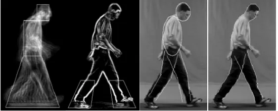
Figure 3-1 Stages of dynamic gait extraction ...33
Figure 3-2 Example fronto-parallel image from a gait sequence ...33
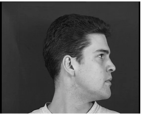
Figure 3-3 Example image for ear recognition ...35
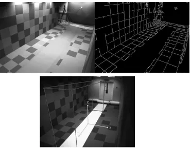
Figure 3-4 Actual and Synthetic Views of the Tunnel ...38
Figure 3-5 Gait Cameras Configuration ...39
Figure 3-6 System Diagram for the Processing Stages...40
Figure 3-7 a) Image From Tunnel b) Edge Detected Image c) Active Volume Projected onto Image ...43
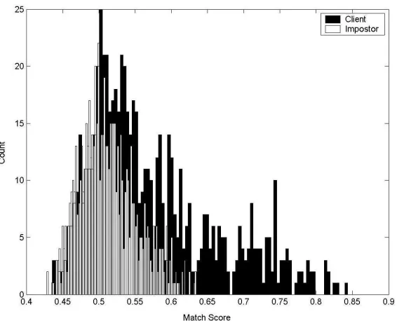
Figure 3-8 Distribution of Client and Impostor Scores for the OmniPerception Face Recognition Algorithm and Matcher ...51
Figure 3-9 Client and Impostor Distributions for Dynamic and Static Gait Distributions Using the Probabilistic Classifer...52
Figure 3-10 Distribution of Client and Impostor Scores for the Ear Modality...53
Figure 3-11 Distribution of Client and Impostor Scores for the Footfall Data...54
Figure 4-1 Receiver Operator Characteristic Curve for Face and Dynamic Gait Fusion ...60
Figure 5-1 An Example Lens Image From the Inspection System ...69
Figure 5-2 System Diagram for Inspection System...71
Figure 5-3 Flow Diagram of Inspection System...72
Figure 5-4 Intensity Profile for a Lens Edge ...73
Figure 5-5 Bubble in Monomer Before and After Extraction...74
Figure 5-6 Edge Fault (a) Before Extraction (b) After Extraction...75
List of Tables
Table 2-1 Equal Error Rates for the Histogram Scaling Experiments...19
Table 3-1 Values Used to Calculate Dataset Size...48
Table 3-2 Values for Number of Samples, Number of Subjects and Number of
Samples Per Subject for Various Expected Error Rates ...48
Table 3-3 Equal Error Rates and Decidability Indices for Modalities Under Test...54
Table 3-4 Timing of System Components ...55
Table 4-1 Equal Error Rates and Decidability Indices for Modalities Under Test
(Repeated) ...58
Table 4-2 Equal Error Rates and Decidability Indices for Fusion of Face and Dynamic
Gait Scores ...59
Table 4-3 Equal Error Rates and Decidability Indices for Combination of All Gait
Modalities ...61
Table 4-4 Equal Error Rates and Decidability Indices for Optimal and Calculated
Weights ...63
Table 4-5 Equal Error Rates, Decidability Indices and Weightings for the Correlation
Experiment...64
Table 4-6 Equal Error Rates and Decidability Indices for Weights Determined by
Predicted Decidability...66
Table 5-1 Fault Types for Edge and Surface Classification ...78
Acknowledgements
I would like to thank my supervisors Mark Nixon and Brian Kett for their
guidance and support during my Engineering Doctorate. I would also like to thank the
staff at Neusciences, especially Trevor Cole, for their involvement in the industrial
inspection work and for agreeing to sponsor my Engineering Doctorate. I am grateful
to John Carter, Lee Middleton, Galina Veres, David Wagg, Silvia Wong and Alex
Buss for their work on the DTC8.11 project that has supported so much of this thesis.
Finally I would like to thank my family and friends for supporting me through these
Definitions and Abbreviations Used
Biometrics Identification of a person by an observed biological or
behavioural characteristic.
Posterior P(C|x) Probability of data coming from a particular class in light of all data.
LikelihoodP(x|C) Probability of observing the data given that the data belongs to the specified class.
EvidenceP(x) Probability of observing data irrespective of the data’s class.
PriorP(C) Probability of observing a particular class irrespective of the data obtained.
Intra-class variance Variance between recorded data belonging to the same
class.
Inter-class variance Variance between recorded data belonging to differing
classes.
Data fusion Combination of multiple sources of information in order
to make a more accurate or more robust decision.
Feature fusion Combination of data sources at the feature level, i.e.
before classification.
Score fusion Combination of data sources at the score level, i.e. after
classification with classifiers providing continuous outputs.
Decision fusion Combination of data sources at the decision level, i.e.
after each piece of information has had a classification assigned.
Balanced classifiers Two or more classifiers where the performance of the
worst classifier is no more than half that of the best classifier.
Imbalanced classifiers Two or more classifiers that do not fulfil the
definition of balanced classifiers.
Score transformation Process of altering scores from disparate classifiers such
that all conform to the same range and distribution.
False match rate Percentage of those impostors who are falsely matched
False non-match rate Percentage of genuine clients who are falsely identified
as impostors at a given threshold, also known as a false rejection.
Equal error rate Percentage value at which the false match rate and false
non-match rate become equal whilst varying the threshold.
Client Genuine enrolled user of a biometric system attempting
to gain authorised access.
Impostor Malicious user of a biometric system attempting to gain
access despite not having permission to do so.
Gait Unique, repeatable, observable pattern produced by a
subject as they walk.
Modality Single biometric method used for identification.
Agent Part of a system that performs information preparation
and exchange on behalf of a client or server.
Voxel Volume pixel, the smallest distinguishable box-shaped
part of a three-dimensional space.
SQL Structured query language.
XML Extendable mark-up language.
Industrial inspection Visual based task of determining faults in manufactured
goods in a production environment.
Commercial of the shelf process control device Device for interfacing
Symbols Used
Chapter 2 (First Use)
P(C|x), P(C|d) Posterior probability given x or d P(x|C), P(d|C) Class likelihood based on x or d P(x), P(d) Evidence of x or d
P(C) Prior probability of class C
N Number of classes
Ci, Cj Class i or j
C The client class
I The impostor class
t Threshold for a verification decision
R Number of classifiers under combination
wi Weight of classifier i Ei Error rate of classifier i Λ Covariance of feature vectors
M Length of feature vector (also number of training examples in eigenface technique leading to feature of length M)
σ2 Variance of feature
Ω Feature vector from eigenface technique
µ Mean of feature
d Distance between new measured feature and reference vector
K Number of example images per class
L Number of likelihoods produced in training set
HL Vector of example likelihoods from training set
HF Mapping vector to a flat histogram of likelihoods
HG Mapping vector to a Gaussian histogram of likelihoods
S(C) Degree of support to a proposition C si Evidence in support of S(C)
Chapter 3 (First Use)
Ψ Average (mean) face
Φ Difference between face image and average (mean) face
A Matrix of training examples
ul Eigenface
U Matrix of all eigenfaces
ωi Component of feature vector
Kj LDA client mean
S LDA between class scatter
Yi LDA class covariance
Σj LDA within class scatter aj Client specific Fisher face
pˆ Measurand error
n Total number of samples
Ns Number of subjects
ng Number of samples per subject
Zij Binary error value
p Expected or desired error value
α Confidence level
d’ Decidability index
Chapter 5 (First Use)
IR Dispersion
Rmax Maximum chord across feature
Rmin Minimum chord across feature
M1-M4 Hu rotation invariant moments (1-4)
ηpq Scale invariant moment order pq
µpq Location invariant moment order pq
Pxy Binary pixel value at location xy
y
Chapter 1
Context and Contributions
1.1
Overview of Research
Probabilistic methods are a group of classification techniques marked by the
fact that their output is a probabilistic measure of similarity between the object under
test and some hypothesised class or classes. The output of this kind of measure
compared with a hard decision or unconstrained score has numerous advantages
explained here. Initially the attraction for such a measure is that it is easily understood
by those using such a system; however the advantages extend beyond the ease of
human utility. For example probabilistic measures are ideal for combination with
other probabilistic outputs since they are guaranteed to be within a fixed range and are
generally well scaled, in certain formulations we may also transparently bias the
classification in favour of certain outcomes. We are interested in examining the utility
of probabilistic methods in two diverse computer vision application domains:
multimodal biometrics and machine inspection.
Biometrics in the automated recognition of a subject by biological or
behavioural characteristics; whilst the field is over fifty years old the majority of this
work has focused on the use of single biological traits, usually termed modalities,
captured in a controlled environment at short range. Recently interest has turned both
to recognition at a distance and the concurrent use of multiple modalities, so called
multimodal biometrics. Recognition at a distance is of obvious benefit in the era of
terms of throughput and of user acceptance where contact devices have proven
unpopular for hygiene and other health related fears. However identification at a
distance often suffers from occlusion and hence strengthens the case for multimodal
biometrics. Investigators of multimodal biometrics have claimed significant
performance improvements over individual modalities in addition to their greater
flexibility. Probabilistic methods are well suited to the combination techniques used in
multimodal biometrics; and in this thesis we examine the utility of these techniques,
the range of their use, technical issues with their implementation and the prediction of
when such techniques should be employed. In order to perform such analysis we have
constructed an automated system for the collection of multimodal biometric data, this
is a highly complex system incorporating significant technical challenges and
considerable research effort. We describe the system, the processing algorithms used,
and the modalities employed; we also describe the collection methodology and the
statistical basis for these decisions.
In comparison with biometrics, machine inspection is a relatively mature field;
however we have examined the sub-field of ophthalmic contact lens inspection at the
request of a commercial organisation. This is field that has had little to no intervention
from complex image processing techniques nor from probabilistic methods.
Ophthalmic contact lens inspection involves the examination of images of contact
lenses on a production line for detection and classification of any faults on the lenses.
Since contact lenses are classified as medical devices the standards for fault tolerance
are very tightly controlled by medical regulators and all decision must be carefully
recorded for subsequent auditing; in addition since inspection takes place in a
production environment processing time is strongly constrained. In this thesis we
develop an automated contact lens inspection system that is suitable for use in a
production environment, we demonstrate the performance of this system and describe
the benefits that complex image processing techniques and probabilistic methods can
bring to this field.
1.2
Contributions
In the field of probabilistic methods these contributions may be summarised as:
1. The use of global variance estimation for homogeneous sets of classes;
2. The modelling of class likelihoods by a logistic function;
3. The formulation of the verification problem as a two class problem modelled
by intra and inter-class logistic functions;
4. The demonstration of a real improvement in both equal error rate and score
distribution by the use of our probabilistic framework;
5. Examination of claims of optimal weighting for probabilistic fusion.
In the field of biometrics these contributions may be summarised as:
1. The development of an automated system for the collection and processing of
multimodal biometric data;
2. The examination of the use of footfall data as a viable modality for biometric
verification;
3. The demonstration of performance improvements using weighted fusion on
highly imbalanced modalities;
4. The examination of the effect of modality correlation on biometric fusion, and
the conclusion that reduction in correlation is a good indicator of improvement
in performance;
5. The demonstration that the decidability index after fusion may be accurately
be predicted, and further more that calculating the maximal decidability
provides an optimal weighing scheme in multimodal biometrics.
In the field of machine inspection these contributions may be summarised as:
1. The development of a system for automatically inspecting medical devices
within a time-constrained environment.
2. The application of complex image processing techniques to ophthalmic lens
inspection;
3. The demonstration of the reliability of our probabilistic classification
1.3
Document Structure
The overall structure separates the industrial inspection application from the
biometrics application, starting with basic probabilistic tenets common to both
application domains.
Chapter 2 provides a background to popular probabilistic techniques and
methods of combining probabilistic confidence measures for different sources. It also
details the theoretical background behind the probabilistic framework we have
developed, which forms an underpinning for the work in the remainder of this thesis.
In the final section of this chapter we perform a comparison between our probabilistic
formulation and Dempster-Shafer theory.
Chapter 3 describes a broad range of novel contributory methodologies,
technologies and systems for biometric recognition that have been used in the Data
Information Fusion, Defence Technology Centre 8.11 (DTC 8.11) contract. Our aim
in the DTC 8.11 contract, that forms the basis of much of the work in this Chapter 3,
was to construct a system for collecting multimodal biometric data from subjects and
automatically verify their identity. Chapter 3 explains the modalities that are targeted
by the system, reviews the background to these modalities and common extraction
techniques before describing in detail the extraction methods we use. It then describes
the collection and verification system we have developed, focusing on the following
areas: the hardware used to construct the system, the pre-processing stages carried out
on the captured data, and the storage solutions for the large volume of data collected.
The collection strategy for our system is explained along with the testing
methodologies we use in the system, as well as detailed descriptions of specific tests.
Chapter 4 examines the simple case of whether score fusion based on our
probabilistic framework is an effective method for improvement of performance. It
then continues, to examine whether multimodal biometrics are an effective tool when
the performance of the modalities are imbalanced. In using the weighted fusion
approximated by the Equal Error Rate; we expand this to examine the role correlation
may have on performance and optimal weighting. Finally Chapter 4 considers the
how we may predetermine any performance improvement we may see and provide a
quantitative assessment of when score fusion is of benefit.
Chapter 5 provides an overview of our developed ophthalmic lens inspection
system including its interaction with the manufacturing equipment and human
operators. This is more industrial in nature than the other work described in this thesis
and fulfils much of the commercial focus elements of the Engineering Doctorate
scheme. This high level overview describes both the inspection system and allied
control and monitoring software. We then describe in detail the methods used for
processing the lens image, extracting relevant feature metrics, classifying fault types
and comparing these classified features with the customer’s inspection standards.
Finally the testing regime that has been implemented is discussed both with reference
to the accuracy of the algorithms and the performance of the system as a whole.
Chapter 6 summarises the findings and contributions made in this thesis. It then
discusses the further work that is desirable to complete outstanding tasks in this thesis
or to provide further development of our key work.
1.4
Publications
The following publications by have ensued from this research programme:
[1] Bazin, A.I., Cole, T., Kett, B., Nixon, M.S. (2006) An Automated System
for Contact Lens Inspection. In Proceedings of 2nd International Symposium on Visual
Computing (ISVC), In Press, Lake Tahoe, NV, USA.
[2] Middleton, L., Wagg, D. K., Bazin, A. I., Carter, J. N. and Nixon, M. S.
(2006) A smart environment for biometric capture. In Proceedings of IEEE
Conference on Automation Science and Engineering, In Press, Shanghai, China. [3] Middleton, L., Wagg, D. G., Bazin, A. I., Carter, J. N., and Nixon, M. S.
IEEE/RSJ International Conference on Intelligent Robots and Systems (IROS), In Press, Beijing, China.
[4] Middleton, L., Buss, A. A., Bazin, A. I. and Nixon, M. S. (2005) A floor
sensor system for gait recognition. In Proceedings of Fourth IEEE Workshop on
Automatic Identification Advanced Technologies, pp. 171-176, Buffalo, New York, USA.
[5] Bazin, A. I., Middleton, L. and Nixon, M. S. (2005) Probabilistic Fusion of
Gait Features for Biometric Verification. In Proceedings of Eighth International
Conference of Information Fusion, pp. 124-131, Philadelphia, PA, USA.
[6] Bazin, A. I. and Nixon, M. S. (2005) Probabilistic combination of static and
dynamic gait features for verification. In Proceedings of Biometric Technology for Human Identification II, SPIE Defense and Security Symposium 5779, pp. 23-30, Orlando (Kissimmee), Florida USA.
[7] Bazin, A. I. and Nixon, M. S. (2005) Gait Verification Using Probabilistic
Methods. In Proceedings of 7th IEEE Workshop on Applications of Computer Vision,
pp. 60-65, Breckenridge, CO.
[8] Bazin, A. I. and Nixon, M. S. (2004) Facial Verification Using Probabilistic
Methods. In Proceedings of British Machine Vision Association Workshop on
Biometrics, London.
The work in [8] describes our initial attempts at constructing a novel
probabilistic framework and this work is described in Appendix B. In [7] we explain
our novel probabilistic framework based on logistic functions, the first such use of
logistic functions in this manner, we demonstrate the performance of this approach on
the gait verification task. Our work in [5, 6] extend our novel probabilistic method
into multimodal biometrics, including the consideration of decidability and correlation
as measures of efficacy; this is the first application directly combining the output of
We describe in [4] a new biometric modality, footfall, and the construction of a
suitable sensor system. The work in [2, 3] explains our work in constructing the first
system for multimodal biometric capture at a distance. Finally [1] gives an overview
of our innovative industrial inspection system utilising modern computer vision
techniques combined with our novel probabilistic framework.
The following publications were also produced by the author during the course
of their Engineering Doctorate, but do not contribute to the content of this thesis:
Damper, R. I., Marchand, Y., Marsters, J. D. S. and Bazin, A. I. (2005) Aligning
text and phonemes for speech technology applications using an EM-like algorithm.
International Journal of Speech Technology, 8(2) pp. 149-162.
Damper, R. I., Marchand, Y., Marsters, J. D. S. and Bazin, A. I. (2004) Aligning
letters and phonemes for speech synthesis. In Proceedings of 5th International Speech
Communication Association (ISCA) Workshop on Speech Synthesis, pp. 209-214, Pittsburgh, PA.
1.5
Declaration
This thesis describes the research undertaken by the author while working
within a collaborative research environment at the Information: Signals, Images,
Systems research group under the support of the Engineering and Physical Sciences
Research Council. This report documents the original work of the author except in:
Chapter 4 which was conducted in conjunction with Drs. Lee Middleton, Galina
Veres, David Wagg and Mr. Alex Buss under the Data Information Fusion, Defence
Technology Centre 8.11 project, and Chapter 6 which was developed in conjunction
Chapter 2
Probabilistic Methods
2.1
Introduction
Probabilistic methods are a group of classification techniques that, when
comparing a piece of query data to a set of possible classifications, produce a
probabilistic measurement of similarity between the query data and each class. This
can be contrasted with the distance based (dissimilarity) metrics or hard classification
(decision) based produced by many other popular classification schemes. There are a
number of obvious advantages with the use of probabilistic methods which return
class assignment with accompanying measures of class certainty, especially in areas
where one may wish to combine disparate sources of data or where one would like
further understanding as the confidence in a classification decision.
This chapter provides a background to popular probabilistic techniques and
methods of combining probabilistic confidence measures for different sources. It also
details the theoretical background behind the probabilistic framework we have
developed, which forms an underpinning for the work in the remainder of this thesis.
In the final section of this chapter we perform a comparison between our probabilistic
2.2
Bayesian Classification
Bayesian classifiers are perhaps the best known method of obtaining a
probabilistic output from a classifier. The naïve Bayesian classifier and its variants [9,
10] have gained interest for use in face recognition [11-15]. The Bayesian classifier
calculates the posterior probability, P(C|x), of a class, C, given data, x. This is based on the likelihood of the data given the class, P(x|C), the evidence of the data, P(x), and the prior probability of the class, P(C), as shown in equation 1.
) ( ) ( ) | ( ) | ( x P C P C x P x C
P = (1)
The prior probability, P(C), is usually assigned such that all classes are equiprobable; and the evidence is taken as the weighted sum of the likelihoods over
all classes:
N C
P( )= 1 (2)
∑
= Nj j j
C x P C P x
P( ) ( ) ( | ) (3)
where i is the number of classes. By combining equations 1, 2 and 3, this leads
to: ) | ( ) | ( ) | (
∑
= N j j i i C x P C x P x CP (4)
Here, x will be a feature vector describing an unclassified object and Ci will be
one possible class identity. In the classification task we assign the data from an
unknown object to the identity Ci if the posterior probability for that class is
) | ( max ) | ( if assign x C P x C P C x k k i i = → (5)
It also aids our future work to consider the more restricted verification problem,
which is more typically used in biometrics. In this problem one already has a claimed
class identity for an object descriptor. Here the object descriptor is an extraction of
measurements of the subject and the class claim provides a claim for the identity of a
single subject. This makes the process somewhat simplified with two possible classes,
either: Client, C, where the individual subject is who they claim to be or Impostor, I,
where they are not. The two classes can be assumed to be equally likely (in the
absence of other evidence) and are mutually exclusive, P(C|x) = 1 - P(I|x). Hence simplifying equation 4 we obtain:
) | ( ) | ( ) | ( ) | ( I x P C x P C x P x C P +
= (6)
We would then accept the individual identity claim if P(C|x) > t where t is a threshold that may be chosen based on the desired security of the system.
The likelihood, P(x|C), will be estimated from the distribution of x for each subject; in many examples [12, 13] this is assumed to be Gaussian distributed. The
multivariate Gaussian for likelihood estimation is given in equation 7; where µi and Λi
are the values for the mean and covariance of the feature vectors of class Ci.
2 1 2 ) ( ) ( 2 1 ) 2 ( ) | ( 1 i M x x i T i e C x P Λ = − Λ − − −
π
µ µ (7)Moghadden et al. [13] argue for two global distributions; one to describe the
distribution of variance between measurements of the same subject (intra-class
variation) and another to describe variation between subjects (inter-class variation). Liu and Wechsler’s work [12] describes only intra-class variation but hypothesises
and the suitability of Gaussian likelihood estimation. We also investigated the
statement by Liu and Wechsler that the posterior probability is not a significantly
better metric than the likelihood.
2.3
Data Fusion
Data fusion may be defined as the combination of two or more feature vectors,
classification schemes or identification decisions with the aim of providing a more
robust estimate of class identity. Fusion may occur on one of three levels [16]:
feature, score or decision. This section will give a brief overview of all methods but
shall focus primarily on score fusion in a probabilistic environment.
For fusion at the feature level, combinations of feature vectors are usually
produced by simple vector concatenation before being passed to a classifier of choice
(usually a simple Euclidean distance classifier), this type of fusion is exemplified by
Kyong’s work on combining face and ears [17]. Whilst this method is simple and
when used with sufficient training data should be optimal, given the usual paucity of
data it is unlikely to be as effective as late fusion. This is especially true if simple
classifiers are used which do not take into account the varying performance of the
modalities being fused. More complex methods may involve the use of feature set
selection or transformation after combination to yield the most discriminant feature
vector [18]. In practice good results from feature level fusion are difficult to achieve
due to incompatible feature types or unknown relationships between feature spaces.
Additionally this technique does not scale well due to increasing demands for more
complex classifiers and increased storage to deal with rapidly expanding
dimensionality.
Decision fusion methods are attractive since they need little or no training and
so cope well with the lack of data often available. Simple decision fusion rules are
merely logical functions such as AND or OR, slightly more complex rules may also
include weighted voting algorithms. Rank based rules [19] such as rank summation,
Borda count or minimum rank can also considered decision fusion schemes. These
methods are simple but do not take into account the scores underlying the initial
inputs or classes. The output of these rules is a hard classification and hence
unappealing in a probabilistic framework or if further analysis may be needed.
Score fusion schemes are broadly of two types: those that regard the output of
the initial classifiers as feature vectors that may be used as inputs to further classifiers
[20, 21]; and those that treat the outputs of the initial classifiers as scores that may be
combined using mathematical rules [19, 22-28].
Many classifiers have been used in score fusion (e.g. support vector machines,
multilayer perceptrons, Bayesian classifiers, Fisher’s linear discriminant analysis
based classifiers and C4.5 decision trees); with Ben-Yacoub et al. [20] claiming that
Bayesian classifiers or support vector machines give the greatest improvement. The
major drawback of using a classifier based fusion scheme is the requirement for
training; in many tasks data is at a premium, especially where many examples of one
class are needed. This lack of training data makes a classifier based fusion scheme
unsuitable for the applications envisaged in this thesis.
Kittler et al. [22] propose a common theoretical framework for the combination
of scores based on the Bayesian decision rule (equation 5), this assumes the
combination of posterior probabilities (or approximations thereof). The rules
described by Kittler are shown in equations 8-12; where P(C|xi) is the posterior
probability from a signal classifier and P(C|x1,…,xR) is the posterior probability from
the R fused classifiers.
Sum rule: =
∑
R
i
i
R P C x
x x C
P( | 1,..., ) ( | ) (8)
Product rule: =
∏
R
i
i
R P C x
x x C
P( | 1,..., ) ( | ) (9)
Minimum rule: ( | 1,..., ) min ( | i) R
i
R P C x
x x C
P = (10)
Maximum rule: ( | 1,..., ) max ( | i) R
i
R P C x
x x C
P = (11)
Median rule: ( | 1,..., ) ( | i) R
R medP C x
x x C
The minimum and maximum rules are approximations to the product and sum
rules respectively; the median rule considers that the sum rule can be considered as
computing the mean posterior probability and hence approximates this behaviour
using the median as a robust estimate of the mean.
The assumption of posterior probabilities poses problems for non-Bayesian
classifiers, especially when attempting to combine classifiers with disparate
distributions of ranges and scores. Where fusion of non-Bayesian classifiers has been
attempted then score transformation techniques have been proposed [19, 21, 29, 30] to
allow these classifiers to fit into the framework proposed by Kittler. It was the
intention of our research to provide a probabilistic framework for data fusion where
score transformation is not necessary; for this reason these methods will not be
discussed further, other than to note that this transformation may introduce further
errors into the classification process.
These rules work well in the case where classifiers are balanced (the error rates
from each classifier are approximately equal); however when classifiers are
imbalanced, use of the sum or product rules can lead to performance that is worse
than the best individual classifier [25]. One solution is the use of
Behaviour-Knowledge Space as proposed by Huang and Suen [31] which formulates a look-up
table to translate classifier outputs to a class label with attached confidence. This
again reduces the fusion to a rank rather than score based system, and requires a very
large training set to populate the knowledge space. A more straightforward solution is
the use of weighted sum and product rules (Linear and Logistic Opinion Pools)
proposed by Benediktsson and Swain [32], these rules are shown in equations 13 and
14.
Weighted sum: =
∑
R
i
i i
R wP C x
x x C
P( | 1,..., ) ( | ) (13)
Weighted product:
i
w R
i
i
R P C x
x x C
where:
∑
=R
i i
w 1 (15)
The setting of the weights, wi, still represents a training requirement but a very
much smaller requirement than other trained methods discussed above. Equation 16
describes the optimal weights, wi, as stated in [25] where Ei is the error in addition to
the Bayes error from classifier i.
k R
i i k
E E w 1 1
1
−
=
∑
(16)
Other methods [33, 34] base the decision to fuse on the perceived expertise of a
given classifier for a given situation. If the classifier is considered an expert then the
decision of that classifier is used, otherwise fusion rules are used that reflect the
confusion over the classification. “Arrogant” classifiers (those that tend towards a
certain decision regardless of collaborating evidence) as described in [34] may be
discounted since they do not yield outputs suitable for combination.
Also of interest are papers describing those situations where classifiers are
suitable for fusion, some interesting rules of thumb appear [19]:
“1. Combining data from multiple inaccurate sensors (having an individual probability of correct inference of less than 0.5) does not provide a significant overall advantage.
2. Combining data from multiple highly accurate sensors (having an individual probability of correct inference of more than 0.95) does not provide a significant increase in inference accuracy.
significant impact in inference capability, because of an added dimensionality of observational data.
4. The greatest marginal improvement in sensor fusion occurs for a moderate number of sensors (i.e., one to seven), each having a reasonable probability of correct identification.”
In addition Daugman [28] states that in the case of imbalanced classifiers the
error rate of the weaker classifier “must be smaller than twice the cross-over [equal
error] rate of the stronger test”. However Roli et al. [25] have demonstrated that the use of the weighted sum rule does give an improvement in performance when fusing
imbalanced classifiers in face recognition. We will seek to explore the accuracy of
these assertions in Chapter 4 since we have the means to test these in a probabilistic
multimodal setting.
2.4
Global Variance Estimation
As described in section 2.2, obtaining accurate likelihoods is dependent on
good estimates of the mean and variance of class data. We are often very constrained
on the availability of data, particularly multiple examples of the same class. Given a
set of M dimensional feature vectors Ω from class Ci, it is trivial to calculate the mean
vector, µi, even from small numbers of examples. However when we attempt to
calculate the covariance matrix of the feature vectors Λi we find that unless the
number of examples used to calculate Λi is greater than M, the covariance matrix is
likely to be singular and hence unsuitable for use in calculations. Where there can be a
reasonable assumption that classes have similar distributions such as in the case of
biometrics; we considered the proposal by Liu and Wechsler [12] that the covariance
could be assumed to be uniform across all classes and further that the covariance
could be considered as a diagonal matrix of the M variances, σ2,of the elements in Ω.
{ , ,..., }
2 2 2 2
1 M
diag
σ
σ
σ
=
For a training set T consisting of K examples from N classes we estimate the variance by subtracting the class mean, µi, from each training vector belonging to
class Ci.
dk = Ωk −
µ
i, k =1,...,K, Ω∈Ci (18)This forms a set of differences D={d1,d2,..,dK} and hence:
∑
=( )
= = K k i ,...,K , kd K σ 1 2 2 1 1 (19)
This then yields a non-singular outcome. Tests on the validity of these
assumptions may be found in the chapter describing biometric data and systems
(Chapter 3). This method would clearly be inappropriate in circumstances where both
the location (mean) and structure (variance) of the data differ greatly between each
class.
2.5
Gaussian Based Likelihood Models
In this section we examine the use of Gaussian based likelihood models for
classification in high dimensional feature space. The multivariate Gaussian likelihood
is given by equation 20:
2 1 2 ) ( ) ( 2 1 ) 2 ( ) | ( 1 i M x
x i T i
e C x P Λ Λ = − − − −
π
µ µ (20)We further found that with no loss of performance we may approximate the
covariance matrix with the diagonal variance matrix as described in 2.4.
In order to test the use of this Gaussian probabilistic frame work, we used the
Principal Component Analysis technique to extract facial feature vectors from a data
centring and cropping to uniform size, transforming to 8-bit greyscale and reducing
them to a 78-dimensional feature space we then constructed training, gallery and
probe sets. We trained the global covariance estimate using 595 images from 119
subjects. We approximated the class means, µi, using a gallery of single images of 200
subjects not used in training the covariance matrix.
From equation 20 we estimated the likelihoods for 200 probe images of the
subjects in the gallery using both the local and global covariance estimates. We then
used equation 4 to calculate the posterior probabilities of each probe image over all
classes and formed an identification decision using equation 5. For comparison we
also used a Euclidean distance classifier for subject identification using the same
probe and gallery sets.
The rank one recognition rate of the Bayesian classifier using a global
estimation of the covariance matrix was 78%; this compares favourably with the
Euclidian distance classifier with a rank one recognition rate of 61%. However,
looking at the probabilistic outputs we realised that there appeared to be a significant
difficulty with Bayesian classifiers that had not been reported in the biometrics
literature. It appears that the likelihoods derived from the PCA data are badly scaled,
spanning fifty or more orders of magnitude, due to the Gaussian functions becoming
very narrow in high dimensions. Likewise the posterior probabilities from Bayes rule
tend to cluster near 0 or 1. These properties could make it difficult to obtain a
reasonable threshold for verification and may reduce the effectiveness of the proposed
data fusion algorithms; they also remove much of the intuitive nature of probabilistic
recognition. This problem appears to be not yet covered in the literature; we suspect
since there has as yet been no consideration of subsequent use of the classification
data, research performance has been satisfied by recognition performance alone.
2.5.1 Histogram Scaling
In order to rectify the problem of poorly scaled outputs we propose a new
method for scaling the likelihoods such that they are well distributed between 0 and 1
[8]. This method is based on using histogram equalisation to map the likelihoods
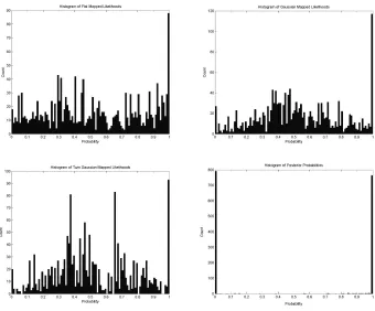
histogram, a Gaussian histogram with a centre at 0.5, and a twin Gaussian histogram
[image:31.595.132.472.135.417.2]with one centre at 0.25 for impostors and another at 0.75 for clients.
Figure 2-1 Results of Histogram Scaling of Likelihoods
Using likelihoods from clients and impostors we form an input vector of length
L,HL, ranked in ascending order. We create two ordered output vectors drawn from
flat, HF, and Gaussian distributions, HG. For the Gaussian distribution the mean, v, is chosen as 0.5 with a variance, s, of 0.25; the length of these two vectors, J, is set so that there may be a unique mapping between the input vector and both of the output
vectors, these are constructed according to equations 21 and 22.
j j ,...,J J
HF(j)= 1 , =1 (21)
j ,...,J
s v j erf
HG(j) , 1
2 1
2 1
=
− +
Each point in vectors HF and HG is multiplied by the number of points, L, in
the example vector HL and rounded down to the nearest integer to give an index for
HL. The value in the mapping vector, M{G|F}, at this point is the value of HL
corresponding to the cumulative variance at the same point in H{G|F}. This provides
us with a mapping from the input histogram to the output histogram, as per equation
23.
M{G|F}(j)=HL(floor(H{G|T}(j)×L)), j=1,...,J (23)
Using this method we also produce a twin Gaussian mapping where two HG
vectors of length J/2 are formed; the first with a centre at 0.25 and the second with a
centre at 0.75. These vectors are then formed into mappings using equation 23 with
the vector HL being drawn entirely from impostors in the first instance, and entirely
from clients for the second mapping. By concatenating these two mappings we form a
mapping HT consisting of two Gaussians trained on client and impostor data.
Again using the Notre-Dame database we performed verification between a
gallery image of a subject and four probe images of the same subject, for each subject
we also presented four impostor images to the system; this test was carried out across
200 subjects in all. For each verification the posterior probability, together with the
flat, Gaussian and twin Gaussian mapped likelihoods were obtained giving four
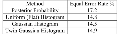
measures of identity for each subject. The EERs for each of these is given in Table
2-1 with the resultant class distributions shown in Figure 2-1.
Method Equal Error Rate %
Posterior Probability 17.2
Uniform (Flat) Histogram 14.8
Gaussian Histogram 14.5
[image:32.595.171.421.571.643.2]Twin Gaussian Histogram 14.9
Table 2-1 Equal Error Rates for the Histogram Scaling Experiments
From our experiment we found that the histogram techniques showed
improvement in verification performance over the posterior probability method. The
posterior probability method at the 1% significance level using a McNemar’s test
however the performance difference between the three histogram techniques is not
significant.
After careful consideration of our findings we decided that a direct method for
calculating the likelihoods without any score normalisation was a more intellectually
robust approach, therefore this work was abandoned in favour of the logistic based
likelihood which coincidentally gave improved results.
2.6
Logistic Function Based Likelihood Models
After initial tests using Gaussian likelihood models for face recognition, we
found that the Gaussian approach did not produce suitable probabilistic outputs for
use in fusion. Since we had set out to construct a schema that directly produced well
scaled probabilistic outputs suitable for use in fusion, it was clearly appropriate to
seek an improved method for likelihood estimation that required no post processing.
When dealing with two class problems, such as biometric verification, there is a
clear advantage in following the methods of Moghaddam et al. [13] in calculating the
evidence based on intra- and inter-class likelihoods, since this significantly simplifies
the calculations.
In keeping with our probabilistic framework we seek to find a function that
tends to unity where the difference between the class mean and feature vector is zero
and tends to zero as the distance between the class mean and feature vector becomes
larger than the class variance.
A suitable model for these distributions is a logistic function [36] such that:
i C i C
b d i
e C
d
P −µ
+ =
1 1 )
|
3 2 2
π
σ
i i C Cb = (25)
Once likelihoods have been calculated for all classes we may then use equation
4 to find the posterior probability for any given class.
For a two class problem such as biometric verification we may make further
refinements to our method. In this case, if we have a distance, d, between a new feature and the feature vector of a claimed identity we wish to calculate the client and
impostor likelihoods, P(d|C), P(d|I), given measurements of the intra and inter-class
means and variances, µC, µI, σC2, σI2. Here we wish the client likelihood to tend to one
as the difference between the new feature and reference vector tend to zero and tend
to zero and the difference becomes larger than the intra-class mean. Conversely we
would wish the impostor likelihood to tend to one when the difference is larger than
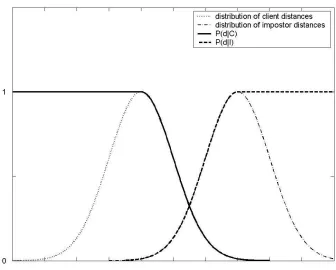
the inter-class mean, and tend to zero as the difference nears zero. If the distributions
of d for clients and impostors are slightly overlapping then the desired behaviour of
the function and the underlying distributions are shown in Figure 2-2. The
overlapping area is that where client and impostor feature sets are of similar distances
from the template; it is within this region that errors occur. The amended functions are
shown as equations 26-28.
C C b d e C d
P −µ
+ = 1 1 ) |
( (26)
( ) I I b d e I d
P − −µ
+ = 1 1 ) |
( (27)
b l l C I
l where |
Figure 2-2 Inter and Intra Class Distributions and Likelihoods
These two functions conform to our requirements set out above that they take
into account knowledge of the variations of d, that they are well distributed and guaranteed to produce outputs between zero and one.
Having found the intra and interclass likelihoods using equations 30 to 32 we
may calculate the posterior probability P(C|d) from equation 6.
Importance sampling [37, 38] could also be used to describe the distribution of
data, however we found that likelihood measures were sufficient to accurately
describe the data so felt this unnecessary.
2.7
Dempster-Shafer Theory
Dempster-Shafer theory [39] provides an alternative probabilistic, which is
our case classes). The belief in a given possibility, Bel(C), is given by combining the
orthogonal sums of all pieces of evidence, mx, in support of this possibility. Belief is
described as “the degree of support a body of evidence provides for a proposition”,
and hence is akin to our view of the posterior probability, P(C|x). Given two pieces of
evidence, s1, s2, for a possibility C; the degree of support S(C) is given by:
S
( )
C =s1⊕s2 =1−(
1−s1) (
− 1−s2)
(33)It is also noted that n pieces of evidence may be pooled using pairwise orthogonal sums:
(
(
(
s1⊕s2)
⊕s3)
...)
⊕sn (34)Should instead we have two pieces of evidence pointing to conflicting beliefs
such as s1 pointing to outcome A and pointing to s2 outcome B, then we erode the
belief in both outcomes:
( )
(
)
2 1 2 1 1 1 s s s s A S − − = (35)( )
(
)
2 1 1 2 1 1 s s s s B S − − = (36)By way of comparison the evidence in our formulation of Bayes rule would be
combined as follows:
( )
2 1 1 s s s A S += (37)
( )
2 1 2 s s s B S += (38)
The authors claim that their method is preferable to Bayes rule in the case of
conflicting evidence for mutually exclusive classes since it retains the “representation
some sway, when compared to our formulation of Bayes rule it also confuses matters
in marginal cases and provides the counter-intuitive situation where our belief in a
complete set of mutually exclusive possibilities does not sum to unity.
2.8
Conclusions
In this chapter we have set out the role of probabilistic techniques in
classification. We have discussed the formulation of Bayes’ rule, which we intend to
use for our probabilistic framework, in order to yield posterior probabilities that we
may make decisions on. We then describe various methods of data fusion, focusing
particularly on score fusion. Having concluded that score fusion has the greatest
potential for our applications, we expand on the use of mathematical rules for score
combination; these rules contain the ability to weight these inputs based on classifier
efficacy. The theoretical optimum for classifier weighting is briefly discussed.
Having set out background techniques we then considered two specific
improvements to our probabilistic framework which dealt specifically with problems
we had identified. Firstly we looked at global covariance estimation for homogeneous
sets of classes in order to overcome a paucity of data. Then we considered the most
appropriate likelihood model for our framework, settling on the logistic function as
especially suitable for the two class problem and those applications with high
dimensional feature vectors. Finally we considered an alternative probabilistic
framework for combining evidence, Dempster-Shafer theory, and highlighted key
differences with our framework.
In future chapters we illustrate the use of these techniques in disparate
application domains and evaluate some of the claims and assumptions that we have
made in this chapter.
In summary our contributions to knowledge from this chapter are:
1. The use of global variance estimation for homogeneous sets of classes;
2. The modelling of class likelihoods by the logistic function;
Chapter 3
Biometric Data and Systems
3.1
Introduction
This chapter describes a broad range of contributory methodologies,
technologies and systems for biometric recognition that could be used in the Data
Information Fusion, Defence Technology Centre 8.11 (DTC 8.11) contract. Our aim
in the DTC 8.11 contract, that has formed the basis of much of the work in this
chapter, was to pioneer a secure access portal to improve building security by
constructing a system for collecting multimodal biometric data from subjects and
automatically verifying their identity.
We have built a ‘tunnel’ environment to aquire multiple biometric modalities at
a distance (at least two metres; such as face and gait, rather than fingerprint or iris).
The tunnel is a self contained system with automatic calibration, subject enrolment,
feature capture and extraction, storage and identification. Automation was considered
important in order to develop a system that could be deployed in a live environment
and also to reduce the very large human burden in collecting a very large biometric
database. The focus on biometrics that may be used at a distance is threefold: firstly
this reduces social factors such as contact with unfamiliar devices that others have
used; secondly these systems may be used covertly and possibly incorporated into
existing surveillance systems; and thirdly subject throughput should be improved
The increased possibility of occlusion or other failures to acquire accurate data
when capturing at a distance is a primary concern leading to the preference of
multiple modalities. By capturing a number of biometric modes we can be more
confident that we have useable biometric samples to identify a subject and often will
be able to combine these to improve identification performance in addition to
reducing failure to acquire rates. In a mass transportation system or other large public
installation, a multi-modal system also provides us an opportunity to include users
who would usually be unable to use a conventional unimodal system due to disability
or cultural sensitivity; since we can select only the appropriate modalities for their use
whilst maintaining reliability for other users.
An equally important aim for this system was to collect a large scale multimodal
database for human identification, at a distance and in a controlled environment.
Collection of a large database of this kind is vital due to the lack of a single source of
biometric data of this kind. This leads to poor quality evaluation data since many
studies restrict themselves to small number of samples and subject created from
amalgam databases where different modalities actually come from different subjects
captured under differing conditions. This leads to myriad problems in effectively
evaluating the data, since one cannot assume that orthogonality of data nor covariate
factors are not artefacts of conflicting experimental protocols between the combined
databases. Uneven protocols between merged databases also rules out many study
types such as those of temporal or environmental effects.
This system is the first multimodal biometric system in the world to be based on
collection of modalities at a distance, there is also contemporaneous work for distance
modalities based on ‘Iris on the Move’ being performed at Sarnoff Corp [40].
We begin this chapter by describing the modalities that are targeted by the
system, we review the background to these modalities and common extraction
techniques before describing in detail the extraction methods we use. We will then
describe the collection and verification system we have developed, focusing on the
following areas: the hardware used to construct the system, the pre-processing stages
by explaining the testing methodologies we use in the system as well as detailed
descriptions of specific tests.
3.2
Modalities
This section describes the modalities that we chose to use in the tunnel. As
explained in the introduction, all of these are capable of automatic capture and
extraction at a distance. For each modality we give a background to the history of the
modality before discussing the technique or techniques that we have selected.
3.2.1 Face
Face recognition from still images is now some 30 years old and a number of
comprehensive review papers have been written describing various techniques to
extract feature vectors [41, 42]. Broadly, techniques may be split into feature based
and holistic techniques, with holistic techniques in the ascendance in recent years. The
baseline holistic technique for face recognition is the eigenface method proposed by
Turk and Pentland [43]. This technique, based on Principal Component Analysis,
transforms an image (of length N2, in vector form), Γ, to a new lower dimensional vector, Ω. Given a set of M training images Γ1, Γ2, Γ3,…, ΓM, the mean face, Ψ, is
given by equation 39, and the difference between each training example and the mean
face is Φi = Γi – Ψ.
∑
=
Γ =
Ψ M
n n
M 1
1
(39)
Since the calculation of eigenvectors from a N2 by N2 matrix would be computationally impossible for typical image sizes, we use a reduced covariance
matrix, ATA, where, A = [Φ1 Φ2 … ΦM], which is of a more manageable size of M by
M. We then find the M eigenvectors, vi, of ATA. These vectors are linearly combined
by equation 40 to form the M eigenfaces, ul, which can also be denoted as a matrix
∑
=
= Φ = M
k
k lk
l v l M
u
1
,..., 1
, (40)
If we sort the M eigenvectors by their eigenvalues in descending order we may
choose to only use the largest few vectors or those that account for a specified
percentage of the variation. This provides a trade off between noise immunity, vector
size and accurate description of the variation. When using the eigenface technique for
recognition, it is useful to ignore the first eigenvector (i.e. that with the largest
eigenvalue) since it typically represents variation in illumination [44].
A new image, Γ, may then be transformed to the new lower dimensional vector,
Ω, where Ω = [ω1 ω2… ωM] and ωk is calculated by equation 41. In this case M is
either the original number of training images or a lower number based on the choices
set out in the proceeding paragraph.
ωk =ukT(Γ−Ψ) (41)
The eigenface technique is by no means the most effective; in comparative tests
it performs 5-10% worse than the best algorithm [45-47]. However it is well
understood and useful for forming a baseline test of face recognition. The eigenface
technique was used in Chapter 2 to test the use of Gaussian models for distribution
estimation. Other still-image techniques of interest are those with a probabilistic or
Bayesian element [11-13, 48-50] and some of these methods have informed our
probabilistic techniques described in Chapter 2.
Pre-processing techniques are also an important factor in face recognition
systems and tools are available to enable this [51]. Face recognition from video is a
more recent area, again of particular interest for our work are those using probabilistic
or Bayesian techniques [52, 53].
Having looked carefully at the eigenface technique with the publicly available
with our other techniques. For this we looked to the Software Development Kit from
OmniPerception Ltd. which grew out of work at the University of Surrey, UK.
The OmniPerception code is based on client specific Fisher faces [54], which builds
upon the work of Belhumeur [55] on Linear Discriminant Analysis for face
recognition. After pre-processing with proprietary algorithms and PCA
dimensionality reduction as described above, the client specific approach used by
OmniPerception proceeds as follows:
Cj is the claimed identity of client j and I is the impostor class. Whilst we are
dealing with the verification problem with a single claimed identity, the impostor
class is built from the other enrolled users in the system during training. If each client
has Mj example images projected into PCA space (Ω j1, Ω j2, … Ω jMj) in the training set
of size M, then the mean for each client Kj is given by equation 42.
∑
= Ω = j M n n j j j M K 1 1 (42)The impostor mean KI based on client j can then be calculated using equation
43, where Ψj is the mean vector for that client. The impostor mean will stay close to
the origin regardless of the client.
j i i I M M M K Ψ − − = (43)
The between class scatter, Sj, for the client-impostor case is given by equation
44.
j Tj
i i
j K K
M M M S − −
= (44)
The covariance of the impostor class, YI, given by equation 46 is related to the