An analysis of pilot whale vocalization activity using hidden Markov models

JASA

An analysis of pilot whale vocalization activity using hidden

Markov models

Valentin Popov∗

School of Mathematics and Statistics,

University of St Andrews, The Observatory,

Buchanan Gardens, St Andrews, KY16 9LZ, UK

Roland Langrock

Department of Business Administration and Economics,

Bielefeld University, Postfach 10 01 31, 33501 Bielefeld, Germany

Stacy L. DeRuiter†

Mathematics and Statistics Department, Calvin College,

3201 Burton SE Grand Rapids, MI 49546, USA

Fleur Visser‡

Behavioural Biology Group, Leiden University,

PO Box 9505, Leiden, 2300 RA, the Netherlands

Abstract

Vocalizations of cetaceans form a key component of their social interactions. Such vocalization activity is driven by the behavioral states of the whales, which are not directly observable, so that latent-state models are natural candidates for modeling empirical data on vocalizations. In this paper, we use hidden Markov models to analyze calling activity of long-finned pilot whales (Glo-bicephala melas) recorded over three years in the Vestfjord basin off Lofoten, Norway. Baseline

models are used to motivate the use of three states, while more complex models are fit to study the influence of covariates on the state-switching dynamics. Our analysis demonstrates the potential usefulness of hidden Markov models in concisely yet accurately describing the stochastic patterns found in animal communication data, thereby providing a framework for drawing meaningful bio-logical inference.

∗ _{Corresponding author.}

† _{Also at: School of Mathematics and Statistics, University of St Andrews, The Observatory, Buchanan}

Gardens, St Andrews, KY16 9LZ, UK

I. INTRODUCTION

Complex patterns of animal communication require appropriate models to resolve the communication process and underlying motivational states. For example, social toothed whales, such as long-finned pilot whales (Globicephala melas), have a complex communi-cation system: individuals typically are highly vocal across the behavioral spectrum and produce a wide variety of call types (Taruski 1979, Sayigh et al. 2013). With the advent of high-resolution on-animal acoustic data recording tags, the potential to study complex communication patterns has strongly increased [Johnson and Tyack 2003]. This is especially true for whales and dolphins, which are otherwise difficult to observe underwater. In turn, increased data availability has raised the question of appropriate models. Methods for mod-eling call rates, particularly in relation to behavior, are not always consistent, and to date the field has not accepted a standard statistical methodology to analyze whale and dolphin sound production rates as a function of behavior state or social respectively environmental context. Methods in most common use range from t-tests, ANOVA and Chi-square tests or non-parametric equivalents to regression models (Deecke et al. 2005, Filatova et al. 2009, Foote et al. 2004, Lemon et al. 2006, Lu´ıs et al. 2014, Oleson et al. 2007, Sjare and Smith 1986), from simple linear models to those incorporating smooth terms, random effects and generalized estimating equations (Quick and Janik 2008, DeRuiter et al. 2013, Di Iorio and Clark 2010, Stimpert et al. 2015, Visser et al. 2016). Other authors use randomization-based methods (DeRuiter and Solow 2008, Miller et al. 2009) or machine-learning classification methods such as random forest decision trees [Henderson et al. 2012]. While some authors have suggested the use of state-switching models for animal call rate data (e.g. Kershen-baum et al. 2014) few studies have pursued this approach to demonstrate its strengths: it deals naturally with the time-series nature of the call rate data, and does not require pre-classification of behavioral states. State-switching models, including the hidden Markov models (HMMs) described here, can in fact provide a comprehensible modern approach to handle the complex biological problem of describing animal vocalization patterns.

not directly observed. This renders HMMs suitable candidates for modeling time series of vocalization rate data. Within an HMM, each observation is assumed to be a realization of one of a finite set of distributions. The different distributions can be interpreted as proxies for the different behavioral states of an individual (or a group of individuals, as many recording methods preclude assignment of calls to individual whales). A Markov chain selects which distribution is active at any time, thereby inducing dependence at the observation level, and in particular allowing for the tendency of particular vocalization behaviors to appear in clusters. The combination of intuitive appeal and mathematical tractability renders HMMs promising statistical tools for the modeling of data on vocalization behavior. Moreover, HMMs allow for the incorporation of additional covariates, which could for example influence the transitioning between states and thus lead to changes in the stochastic description of the vocalization activity.

HMMs are becoming increasingly popular in ecology, having been applied, inter alia, to animal movement data (see, e.g., Langrock et al. 2012), to accelerometer data from animal-borne data-loggers (see, e.g., Broekhuis et al. 2014) in capture-recapture studies (see, e.g., Johnson et al. 2016), within distance sampling, (see, e.g., Borchers et al. 2013), to occupancy data (see, e.g., Gimenez et al. 2014), to data on feeding behavior (Schliehe-Diecks et al. 2012) and to data on diving behavior of whales [DeRuiter et al. 2016].

Our main aim is to make inferential statements about the stochastic structure of the vocalization activity of pilot whales, including in particular the potential effect of relevant explanatory variables related to their social behavior. In the pursuit of this aim, we describe in detail a general method for modeling animal communication data, which provides a powerful addition to the tool kit of bioacousticians and ethologists.

II. DATA

param-eters of the tagged whale’s group were recorded by two dedicated observers on the research vessel, which was following the whales at a distance of 100-400 m. This resulted in a total of 7 data sets ranging in duration from 40 minutes to 9 hours. Due to the long intervals between tagging events, the data sets can reasonably be assumed to be independent.

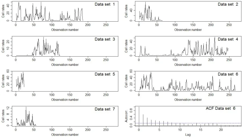
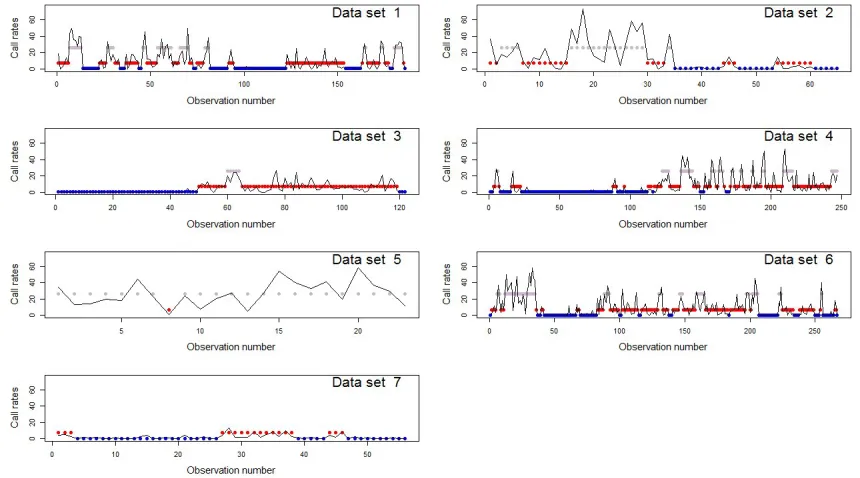
The stereo sound recordings from the DTAGs (16-bit resolution at 96 or 192 kHz) were used to analyze the patterns in whales’ vocal behavior. Call start times were identified visually in spectrograms (Blackman-Harris window, 4096 sample FFT, 75% overlap, 180 dB dynamic range) by experienced analysts, marked using Adobe Audition 2.0, and the total number of calls per 2-minute interval was recorded.

FIG. 1: Call rates of whale calls by data set. Thex−axis gives the observation number of the 2-minute intervals. Bottom right plot shows the empirical autocorrelation function

(ACF) of the whale call counts for the 6th data set. The dotted blue line gives a 95% confidence interval for the expected value of the ACF in the case of independent

observations.

a very short period the record approaches a simultaneous sample of all individuals (Altmann 1974). These parameters, quantifying the degree of group aggregation, cohesion and surface activities, are: 1) group size, 2) number of individuals in the focal area, 3) number of groups, 4) distance to the nearest other group (6 categories: <50 m, 50-100 m, 100-200 m, 200-500 m, 500-1000 m, none in sight), 5) individual spacing (distance between individuals in the focal group; 5 categories: very tight (< 1 body lengths (BL)), tight (1-3 BL), loose (3-15 BL), very loose (> 15 BL) and solitary (no other individual in focal area and/or distant from nearest neighbor)), 6) logging (in which a whale floats at the sea surface; 2 categories: absent, present), 7) spyhops (in which a whale’s head emerges vertically from the water; 2 categories: absent, present), 8) synchrony (3 categories: low, medium, high) and 9) milling (in which whales swim slowly and without a consistent direction at the surface; 2 categories: absent, present). Parameters were recorded at 2-minute intervals, or at first surfacing of the tagged individual following dives longer than 2 minutes. Hence, group-level behavior was sampled when the tagged individual was visible at the surface. See Visser et al. [2014] for more details on the focal follow protocol.

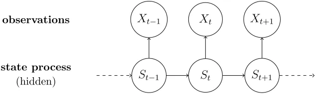
state process

(hidden) St−1 St St+1

observations Xt−1 Xt Xt+1

FIG. 2: Visualization of an HMM. Arrows indicate dependence. Here, the state process S is the behavioral state of the whales, and the observations X are calls per time interval,

with subscripts indicating the time period.

III. MODEL FORMULATION AND STATISTICAL INFERENCE

An HMM consists of two components: an observable time series and an underlying latent state sequence. The observable time series for a single data set, denoted byXt,t= 1, . . . , n,

in our case relates to the counts of whale calls. Each observation, i.e. each count of calls per given time interval, is assumed to be the realization of one ofN distributions. We will assume that the N state-dependent distributions are from the family of negative binomial (NB) distributions because it can handle overdispersion within the state-dependent distribution. The state process, denoted by St, t = 1, . . . , n, takes values from 1 to N and determines

which of the N distributions the observation Xt is drawn from. The choice of N can be

based on formal model selection criteria, pragmatic considerations or a combination of both; see Section III.D. The Markov property is assumed for the state process, so that that St

depends only on the previous state variable St−1. The two components of an HMM with their dependence structure are visualized in Figure 2.

A. Baseline model

in the N ×N transition probability matrix (t.p.m.):

Γ= 

   

γ11 ... γ1N

..

. . .. ...

γN1 ... γN N



   

.

Note thatPN

j=1γij = 1 for all i= 1, . . . , N, that is, each row of the t.p.m. sums to unity. Particularly in the ecological literature, Bayesian inference based on Markov Chain Monte Carlo sampling has often been implemented for the purpose of estimating the parameters of state-switching models conceptually similar to the one defined above, especially in the field of animal movement modeling; influential examples include the work of Morales et al. [2004] and Jonsen et al. [2005]. While certainly feasible in many cases, such approaches tend to involve a very high computational cost, rendering the analysis of longer time series very time intensive. We discuss and implement a maximum likelihood approach instead, primarily because of the associated low computational cost (but see the discussion section). In order to calculate the likelihood of an observed time series x1, . . . , xn, all possible state

sequences that might have given rise to the observations need to be considered. A brute force approach, separately considering all Nn possible state sequences, is clearly not feasible in general. Fortunately, there is a much more efficient way of considering the different trajecto-ries the state process might have taken, namely via the application of the recursive scheme called the forward algorithm (see, e.g., Zucchini et al. 2016). This algorithm effectively traverses along the time series, updating the likelihood at every step while maintaining all relevant information on the state process. In particular, it uses the forward probabilities, defined as:

Exploiting the dependence structure, we see that these can be recursively updated:

αt(i) =Pr(Xt =xt|X1 =x1, ..., Xt−1 =xt−1, St =i)Pr(X1 =x1, ..., Xt−1 =xt−1, St =i)

=Pr(Xt =xt|St =i) N

X

k=1

Pr(X1 =x1, ..., Xt−1 =xt−1, St−1 =k, St=i)

=Pr(Xt =xt|St =i) N

X

k=1

Pr(St =i|X1 =x1, ..., Xt−1 =xt−1, St−1 =k)

×Pr(X1 =x1, ..., Xt−1 =xt−1, St−1 =k)

=

N

X

k=1

αt−1(k)γkiPr(Xt =xt|St =i),

which in matrix notation gives the forward recursion

αt=αt−1ΓP(xt),

where P(xt) is an N ×N diagonal matrix with the conditional probability mass functions

pi(xt) = Pr(Xt=xt|St=i),i= 1, ..., N, on the main diagonal. The initial calculation is

α1 =δP(x1),

where δ is a row vector with the initial state distribution of the Markov chain.

Repeated application of the forward recursion constitutes the forward algorithm, which leads to the following matrix product expression for the likelihood:

L(θ|x1, ..., xn) = δP(x1)ΓP(x2)×...×ΓP(xn)1,

where 1 is a column vector of ones and θ denotes the vector with the parameters to be estimated. For the baseline model these include the N ×(N −1) transition probabilities and theN ×q parameters of the N state-dependent distributions with q parameters each.

In our specific example, we assume that pi(xt) is a negative binomial distribution

proba-bility mass function with q= 2 parameters — state-specific size, ni, and mean, µi, i.e.:

pi(x) =

Γ(x+ni)

Γ(ni)Γ(x+ 1)

ni

ni+µi

ni

µi

ni+µi

x

Here Γ(·) denotes the gamma function. For a homogeneous state process, it is usually ade-quate to assume that the process is in equilibrium, also called “steady state”, when we start observing it, since the actual behavioral process will already have been active for quite some time. The initial distribution then is assumed to be the equilibrium (stationary) distribution. In this caseδ can be calculated as the solution to the equation systemδ(IN −Γ+U) =10,

where IN is an N ×N identity matrix and U is an N ×N matrix of ones [Zucchini et al.

2016]. The homogeneity assumption will however be relaxed in the next section, in which case δ will need to be estimated.

To illustrate how the likelihood function is constructed, consider a two-state HMM with t.p.m.

Γ= 



1−γ12 γ12

γ21 1−γ21 

.

Suppose that the two state-dependent distributions are negative binomials withpi(x) given

in (1), with parameters (µ1, n1) and (µ2, n2), respectively. When the Markov chain is in equilibrium at the start of the time series, then δ = 1/(γ12+γ21)(γ21, γ12) (the stationary distribution). In the first data set the call rates are given by (19,0,. . .,0) (where the dots do not indicate zeros, but general observations which we do not detail here for reasons of space). The corresponding likelihood is:

L(θ|19,0, ...,0) = 1

γ12+γ21

(γ21, γ12)





p1(19) 0 0 p2(19)





×





1−γ12 γ12

γ21 1−γ21



 



p1(0) 0 0 p2(0)



 . . . 



1−γ12 γ12

γ21 1−γ21



 



p1(0) 0 0 p2(0)

    1 1  ,

where θ= (γ12, γ21, µ1, n1, µ2, n2)0.

To fit an HMM of the type described above, we first assume that the data from the seven tags are generated by the same stochastic process, i.e. we pool the information from the seven tags and fit a single model to them, assuming parameters to be identical across the different series observed. This is a strong simplifying assumption, which could be relaxed in cases where longer time-series of data are available for each individual (or group) under observation (DeRuiter et al. 2016, Zucchini et al. 2016).

is the sum of the seven individual log-likelihoods. This joint log-likelihood is maximized numerically, using Newton-Raphson-type optimization in the statistical software R, using the routine nlm() [R Core Team 2016].

B. A model with covariates in the t.p.m.

When considering covariates in an HMM, it is usually preferable to assume that the external variables influence the transition between states rather than the state-dependent distributions, which remain fixed for a given state. Otherwise the interpretation of the states can become very difficult, as different levels of the covariates would lead to varying shapes of the state-dependent distributions, potentially making it very difficult to regard the HMM states as proxies for behavioral states [Zucchini et al. 2016].

The row constraints on the t.p.m., i.e. γij ∈[0,1],

PN

j=1γij = 1, for i = 1, . . . , N, can be

dealt with by using a multinomial logistic link function:

γij =

exp(β_ij0 yt)

PN

l=1exp(β 0

ilyt)

, (2)

where y0_t = (1, y1,t, ..., yk,t) is a vector with the k covariates at time t and βij is a k + 1

column vector with coefficients to be estimated. Note that multiplying the numerator and the denominator in (2) by a suitably chosen non-zero constant would yield a different set of parameters β without changing the transition probability. Thus, for identifiability reasons, we set βii = 0 for i = 1, . . . , N — this is standard practice in multinomial logit modeling

(McFadden 1984). The number of parameters in the t.p.m. increases compared to the baseline model fromN·(N−1) to N·(N−1)·(k+ 1). The baseline model is a special case of this model, in which all covariate coefficients are zero. Note that when covariates influence the transition probabilities, the Markov chain is no longer homogeneous. In particular, we can no longer assume the state process to be stationary, so the initial state distribution needs to be estimated together with the other model parameters. Apart from the change in the construction of the t.p.m., the calculation of the log-likelihood function and its maximization proceed as described above.

provide some information about the whales’ underlying behavioral state (or more specifically, the likelihood that they will transition between states). We next consider transformations of the available covariate data.

C. Aggregating covariates

All the covariates considered in this analysis come from the focal follow data. As men-tioned in Section II in total there are 9 social behavior metrics of potential interest: Group size,Number in focal area,Number of groups,Distance to the nearest group,Number logging, Number of spyhops, Spacing, Synchrony and Milling. Inclusion of such a large number of variables would lead to heavily parameterized models, which in turn leads to model fitting limitations given the moderate sample size of call rates. In addition, the covariates are unlikely to be fully independent of one another, so including all of them is not efficient in terms of number of parameters required to improve the model fit, while still allowing for biologically meaningful inference. One way to cope with this problem is to use multivariate data analysis methods to aggregate the data in such a way that a large amount of the in-formation from the social behavior parameters is preserved, while the number of variables is reduced. Before aggregation, we first divide the 9 variables into clusters, which relate to different aspects of the whales’ behavior. The goal is to create a synthetic variable for each cluster and in that way to reduce the dimensionality of the data.

In particular, we consider three groups:

• Aggregation(mixture of quantitative and categorical variables): Group size (integer-valued);Number in focal area (integer-valued);Number of groups (integer-valued) and Distance to the nearest group (categorical)

• Surface activities(both variables are binary): Loggings and Spyhops

• Cohesion (all variables are categorical): Spacing,Synchrony and Milling

method has Principal Component Analysis (PCA) and Multiple Correspondence Analysis (MCA) as special cases. It is implemented using the function PCAmix from the R package

PCAmixdata [Chavent et al. 2014].

The resulting synthetic variable is labeledAggregation. A problem associated with this synthetic variable is that, like all PCA results, its values can be difficult to interpret.

The synthetic variable forSurface activitiesis created in a simple way. It is constructed by adding the two binary variables. Consequently, it takes the value 2 if both logging events and spyhops are observed, 1 if only one of these is observed and 0 otherwise. In that way this synthetic variable has a simple interpretation (no activity, one activity or two activities).

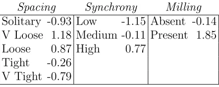
A similar procedure to that used for Aggregation is applied to Cohesion. However, since the cluster contains only categorical variables, a standard MCA is applied. Using generalized singular value decomposition of the centered indicator matrix of the levels of the variablesSpacing,Synchrony and Milling, the standard MCA assigns a coefficient (loading) to each factor level [Chavent et al. 2014]. In that way, the synthetic variable Cohesion is built as a sum of the three coefficients for each combination of factor levels of the three variables. Table I gives the coefficients (rounded to 2 digits) from the MCA.

Spacing Synchrony Milling Solitary -0.93 Low -1.15 Absent -0.14 V Loose 1.18 Medium -0.11 Present 1.85 Loose 0.87 High 0.77

Tight -0.26 V Tight -0.79

TABLE I: Coefficients from the MCA. For each combination of factor levels, e.g. ‘V Loose’, ‘Low’, ‘Absent’, the synthetic variable Cohesion equals the sum of the respective

coefficients.

For Cohesion, the results can be interpreted as follows. For fixed values of Spacing and Milling, an increase in the degree of synchrony observed will lead to an increase of the synthetic variable. On the other hand, for fixed values of Milling and Synchrony, tighter group spacing will decrease the value of Cohesion.

In addition to the three synthetic variables, we also consider the variableSpacing from the original dataset as a potential covariate. The goal is to assess the gains (in terms of model fitting) of using the synthetic variable as opposed to using a single variable from the cluster. Additionally, for the Spacing covariate we consider a “time to change” (TTCh) variable. It measures the absolute value of time (in minutes) to the nearest change in group behavior (whether the nearest change occurs before or after the current time-bin). The idea behind the introduction of such a variable is that the whales may change their communication intensity both before and after a change in behavior, in order to coordinate their behavior before, during and after the change. (TTCh variables could potentially be defined for the synthetic variables as well, but like the synthetic variables themselves will be more difficult to interpret.)

D. Model selection

In order to choose between different candidate models, we consult two model selection criteria. The first one is the Bayesian Information Criterion (BIC), BIC = −2 log` +

plogntot, where log` is the joint log-likelihood for the seven data sets, p is the number of parameters estimated, i.e. the length of the vector θ, and ntot is the total number of observations, 966 in our case.

In ecological applications, formal model selection approaches tend to favor fairly complex models, in particular those with numbers of states that are often higher than would be expected a priori. For example, some states may be included essentially only as a way of compensating for the relative simplicity of the model formulation, compared to the actual ecological process. An example of this phenomenon is described in Langrock et al. [2015], where simple parametric state-dependent distributions were not flexible enough to capture the shape of the patterns observed within clearly defined, biologically meaningful states, hence leading to an overly complex state architecture (with seven states, where three or four seemed much more biologically reasonable). Standard model selection criteria such as BIC may also fail to identify a suitable, biologically reasonable number of states in the presence of within-day variation which is not explicitly accounted for in the model, or a non-Markovian correlation structure of the state sequence. Therefore, while considering formal model selection criteria, we also rely on biological intuition and pragmatic considerations.

E. Model checking

In addition to applying model selection criteria to select a model, we use ordinary pseudo-residual plots to assess the goodness-of-fit of the HMM. Following Zucchini et al. [2016], for an observation xtwe calculate the respective normal pseudo-residual segments [zt−, z

+

t ] with

z_t−= Φ−1 Pr(Xt< xt|X−t =x−t

and

z_t+= Φ−1 Pr(Xt≤xt|X−t=x−t

,

where Φ(·) is the cumulative distribution function of the standard normal distribution, x−t

is a vector of all observations except for xt and X−t is defined in a similar way in terms of

the random vector of process variables.

When xt= 0, i.e. the smallest value an NB distributed random variable can take, we set zt−

F. Interpretation of the parameters in the t.p.m.

For the model with covariates in the t.p.m., a direct interpretation of the parameters in βij is not straightforward because the effect of the covariate on the transition probabilities is a nonlinear function of the parameters in the t.p.m. A pairwise comparison of the transition probabilities in each row is possible, for example using odds ratios. However, the latter do not provide information about the net effect of the covariate on the probabilities. In our view, a more informative approach in describing the effect of a covariate on the t.p.m. is to examine the stationary (or equilibrium) distribution assuming the covariate is fixed at a certain level [Patterson et al. 2009]. This provides information on the marginal behavior of the model given the chosen value of the covariate and the estimated coefficients. Comparing the results for different fixed levels allows us to draw conclusions about the influence of the respective covariate. Confidence intervals for the stationary distributions can be calculated using the delta method [Oehlert 1992]. More precisely, for the asymptotic variance of the estimateδˆconsidered as a function of a vector with all estimatedβij coefficients, sayβ, andˆ

a value of the covariatey, we have

V ar(δˆ)≈f0(βˆ, y)>V ar(β)ˆ f0(βˆ, y), where

f(βˆ, y) =1>IN −Γ(βˆ, y) +U

−1

with the entries in Γ(βˆ, y), a function of the estimated parameters βˆ and y, given in (2). ˆ

β is asymptotically normally distributed and so isδ. The derivativesˆ f0(βˆ, y) can be calcu-lated numerically, whereas V ar(β) can be estimated by inverting the Hessian matrix of theˆ parameters.

We can also calculate the transition probabilities for set covariate values, in order to gain insights about how likely the whales are to switch states under certain conditions.

G. Viterbi algorithm

conditional probability:

Pr(S1 =s1, ..., Sn =sn|X1 =x1, ..., Xn =xn)

or, equivalently:

Pr(S1 =s1, ..., Sn=sn, X1 =x1, ..., Xn=xn)

Viterbi is a recursive algorithm for solving this optimization problem [Zucchini et al. 2016]. The state sequences underlying the seven data sets can be decoded separately, due to the independence assumption.

IV. RESULTS

A. Baseline models

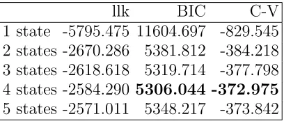
As a preliminary step towards fitting our main model, we fit NB HMMs with up to 5 states. The aim is to gain a rough idea of the number of states before we consider covariates in the models. Table II provides a summary of the model selection criteria for the 5 fits. Comparatively small values of the BIC and, respectively, comparatively large values of the cross-validated (log) likelihood indicate a better fit.

llk BIC C-V

1 state -5795.475 11604.697 -829.545 2 states -2670.286 5381.812 -384.218 3 states -2618.618 5319.714 -377.798 4 states -2584.290 5306.044 -372.975 5 states -2571.011 5348.217 -373.842

TABLE II: Model selection criteria for benchmark models with no covariates; llk gives the maximum log likelihood, while C-V stands for mean cross-validated (log) likelihood.

et al. 2008]. Second, examining the maximum-likelihood values in Table II, the greatest improvements in terms of the goodness of fit are obtained up to the 3-state model. For more than three states the likelihood further increases but at much smaller rates. Finally, given the relatively short lengths of the individual time series, including covariates in HMMs with more than three states renders corresponding models very unstable numerically. It leads to high variances of the parameter estimators, due to the high complexity of the model relative to the number of observations available. While fitting a baseline model, without covariates, is still feasible given the relatively small sample size, this is not the case with the more complex model formulations presented below. A 3-state model therefore seems to provide a reasonable compromise between the result of the formal assessment of the models and practical considerations.

B. Models with covariates

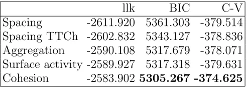
We fit five 3-state NB models, each with one covariate: either spacing, spacing TTCh or one of the three synthetic variables. Conceptually it would be straightforward to extend our model formulation to fit models with additional covariates, but given the small size of the current data set, we limited ourselves to one covariate at a time to avoid numerical instability in the fitting process. Results are given in Table III.

llk BIC C-V

Spacing -2611.920 5361.303 -379.514 Spacing TTCh -2602.832 5343.127 -378.836 Aggregation -2590.108 5317.679 -378.071 Surface activity -2589.927 5317.318 -379.631 Cohesion -2583.902 5305.267 -374.625

TABLE III: Model selection criteria for 3-states NB HMM models with 1 covariate. llk gives the maximum log likelihood, while C-V stands for mean cross-validated (log)

likelihood.

brings improvement in the fit as opposed to considering only one variable from the cluster. To support this statement, we additionally fitted models with onlySynchrony and Milling, respectively. We do not report the results here to keep the overview of the models simple, but note that no individual covariate improved the fit compared to the model with the cor-responding synthetic variable. We note that, according to both model selection criteria, the TTCh (time to change in Spacing) variable results in a considerable improvement compared to Spacing, which underlines the potential importance of TTCh variables.

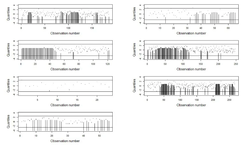
Before considering the fitted model and associated interpretations in more detail, we assess the fit using pseudo-residuals (Figure 3). There are very few outliers and no clear patterns over time, and thus no evidence of any notable lack of fit.

FIG. 3: Pseudo-residual segments in each data set. Thex−axis gives the observation number of the 2-minute intervals. Here α is set to 1% and the solid lines give the 99.5

%-and the 0.5%-quantiles of the st%-andard normal distribution. Intervals going to −∞ have been truncated to −4 to facilitate plotting.

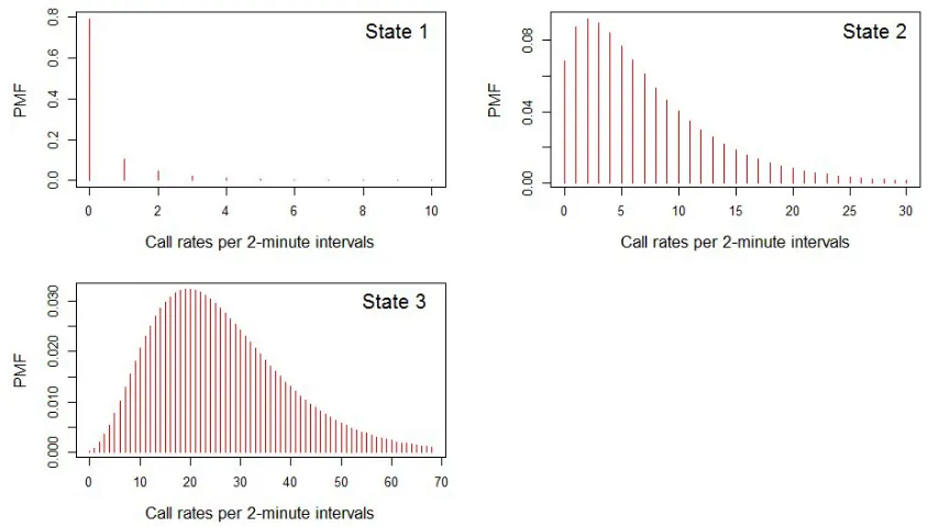
Size Mean State 1 0.1932 0.4479 State 2 1.5648 7.1295 State 3 4.2105 26.2091

TABLE IV: Estimates of the size and mean parameters in the 3-state NB distribution with Cohesion as covariate

FIG. 4: PMFs of the state-dependent distributions in the 3-state NB distribution with Cohesion as covariate.

The estimated covariate-dependent t.p.m. is

tΓ =

          1

1 + exp(η(₁₂t)) + exp(η₁₃(t))

exp(η(₁₂t))

1 + exp(η₁₂(t)) + exp(η₁₃(t))

exp(η₁₃(t))

1 + exp(η₁₂(t)) + exp(η(₁₃t)) exp(η₂₁(t))

exp(η₂₁(t)) + 1 + exp(η₂₃(t))

1

exp(η₂₁(t)) + 1 + exp(η₂₃(t))

exp(η₂₃(t))

exp(η(₂₁t)) + 1 + exp(η(₂₃t)) exp(η₃₁(t))

exp(η₃₁(t)) + exp(η₃₂(t)) + 1

exp(η(₃₂t))

exp(η₃₁(t)) + exp(η(₃₂t)) + 1

1

exp(η(₃₁t)) + exp(η₃₂(t)) + 1           , where

η(₁₂t)=−2.1105 + 1.0252yt; η

(t)

13 =−4.2765 + 0.5212yt; η

(t)

21 =−2.1869 + 0.0880yt;

with yt giving the value of the Cohesion variable at time t.

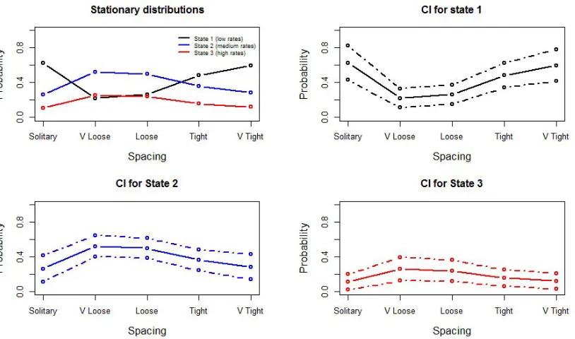
As mentioned earlier, a direct interpretation of the Markov chain parameters is difficult. Therefore, we examine the stationary distributions and the transition probabilities for fixed levels of Cohesion as suggested in Patterson et al. [2009]. The choice of values at which to fix the Cohesion variable is based on the data. In particular, we observe that in 562 out of 966 observations (around 60%), Synchrony takes the value ‘Medium’ and Milling is ‘Absent’. Thus, for the calculation of the synthetic variable we fix Synchrony and Milling to these levels and allow only Spacing to vary. In that way we examine the behavior of the stationary distribution and the t.p.m. for all five different levels of Spacing.

We start with the stationary distribution (Figure 5).

FIG. 5: Stationary distributions and confidence intervals for different values of spacing, synchrony and milling fixed to medium and absent, respectively.

close to one another.

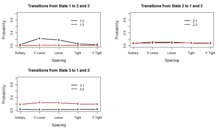
FIG. 6: Between-state transition probabilities for different values of spacing, synchrony and milling fixed to medium and absent, respectively.

The rates of transition between states are given in Figure 6. When whales are in the medium- (state 2) or high-call-rate states (state 3), the between-state transition probabilities change little when spacing changes. On the other hand, the probability of switching from state 1 to state 2 seems to be heavily influenced by spacing. In particular, it takes a relatively high value (23.4%) when the whales are very loose, but drops drastically (4%) when the whales are close to each other. Overall, the pilot whales are more likely to leave the low-call-rate state when they are very loosely spaced, and much more likely to stay in this relatively-silent state when they are tightly spaced.

state 3. Consequently the whales do not seem to have a preferred state, however they tend to spend twice as much time in the states with low and medium vocalization compared to the state with high vocalization.

V. DISCUSSION

HMMs can be used for classification purposes as well as to draw inferences from the time series data. A detailed discussion of the differences in these two types of applications is provided in Leos-Barajas et al. [2016]. While past studies on toothed whales have concen-trated on the former type of application [Brown and Smaragdis 2009, Clemins and Johnson 2005, 2009, Miller and Isojunno 2013], the focus of this paper was on the latter. In par-ticular, we aimed at (i) describing the structure of the data-generating process, in addition to (ii) making inferential statements about the transition between behaviors in relation to covariates.

In the pursuit of (i) our methodological approach involved deciding on the number of states in the HMM instead of fixing it a priori. The choice of a 3-state HMM was partly driven by the data, yet still took into account practical as well as biological considerations. We labeled the three states identified by the HMM as low, medium and high call rates, respectively, according to the mean calls produced in each state, but did not associate them with behavioral states. As noted in Leos-Barajas et al. [2016], HMMs are only an approx-imation of the true data-generating process. Consequently, nominal HMM states may or may not have a biologically meaningful interpretation. We note that there is evidence in the literature that different behavioral categories are associated with different call rates. For example, Taruski [1979] finds a significant difference between the mean call rate pro-duced during milling and the mean call rate propro-duced during transiting. Taruski [1979] also attempts to classify the behavior of pilot whales in three states depending on the level of arousal (low, moderate and high) but concludes that “the concept of arousal level is an inadequate explanation of the variations in [...] calling rate”. It is thus reasonable to assume that the three HMM states relate to complex sets of behavioral categories, but without a strict correspondence between particular call rates and specific behaviors.

members, and synchronize behavior.

Further support for our findings is provided in Weilgart and Whitehead [1990]. Study-ing different types of pilot whale calls, the authors found significantly positive correlation between most call types and the size of the area over which the focal group was scattered. Thus more calls were produced when the whales were spread over a larger area.

A challenge in the present work was to include as much information as possible from the (relatively large) set of covariates available. The moderate sample size, relative to the number of model parameters and potential covariates, posed fitting limitations. In particular, the chosen 3-state HMM limited the number of covariates that can be included in the model to one. We used MCA, among other methods, to compact part of the covariate data into one synthetic variable. This synthetic variable, Cohesion, provided an adequate fit, while outperforming other candidate models.

In the course of the analysis we investigated another variable of potential interest, namely time to change (TTCh) in group spacing. TTCh was shown to be a better predictor of changes in behavioral state than the underlying behavioral variable (Spacing) but still infe-rior (in terms of model fit) to the synthetic variableCohesion. Richer data sets which allow the fit of HMMs with more than one covariate could better elucidate the relative importance of TTCh. However, the initial findings of our study illustrate that call rates vary with social context, with more frequent communication needed not only in association with particular activities and characteristics of the social group, but also at times when those activities or characteristics are shifting.

Our set of covariates consisted of a limited number of social behavioral variables. Other studies have demonstrated the influence of additional variables on the vocalization of del-phinids. For example, traveling speed is a variable of potential interest [Henderson et al. 2012]. However, including relevant information in the framework of HMMs from a wider set of covariates is a challenging task, which is left for further research.

Bayesian framework also comes with technical challenges such as label switching. More importantly, it often involves very slow mixing of Markov Chain Monte Carlo samplers, and model fitting may require days or weeks of computing time. In our experience, maximum likelihood estimation of HMMs tends to be magnitudes faster (see also Zucchini et al. 2016). This was also the main reason for using maximum likelihood estimation within the R package ‘moveHMM’, which is tailored to analyzing animal movement data using HMMs [Michelot et al. 2016]. Bayesian estimation of the number of states adds a further challenge [Zucchini et al. 2016]. In general, in the absence of a need to incorporate informative prior information in the model, and as long as the likelihood of the desired model can be readily evaluated numerically, a maximum likelihood approach such as the one presented here can be an efficient, effective way to fit HMMs.

HMMs have proven to be an extremely useful tool for modeling animal behavior, and the current paper adds to the increasing literature of successful applications of the models in statistical ecology. HMMs are well suited to modeling scenarios where hidden motivational states drive an observable aspect of animal behavior, in this case the communication within a group of pilot whales measured as call counts. They provide both analytical tractability and the flexibility to modify the baseline model (for example, by including covariates affecting the between-state transition probabilities). For these reasons, HMMs can provide a nuanced quantitative description of animal behavior data, and may prove particularly useful in studies relating sound-production rates to broader behavioral states.

ACKNOWLEDGMENTS

Altmann, J. (1974) Observational study of behavior: sampling methods, Behaviour, 49(3), pp. 227–266.

Borchers, D. L., W. Zucchini, M. Heide-Jørgensen, A. Ca˜nadas, and R. Langrock (2013) Using hidden Markov models to deal with availability bias on line transect surveys, Biometrics, 69(3), pp. 703–713.

Broekhuis, F., S. Gr¨unew¨alder, J. W. McNutt, and D. W. Macdonald (2014) Optimal hunting conditions drive circalunar behavior of a diurnal carnivore, Behavioral Ecology, pp. 1268–1275. Brown, J. C. and P. Smaragdis (2009) Hidden Markov and Gaussian mixture models for automatic call classification,The Journal of the Acoustical Society of America, 125(6), pp. EL221–EL224. Celeux, G. and J.-B. Durand (2008) Selecting hidden Markov model state number using cross-validated likelihood, Computational statistics, 23, pp. 541–564.

Chavent, M., V. Kuentz-Simonet, A. Labenne, and J. Saracco (2014) Multivariate analysis of mixed data: The PCAmixdata R package, arXiv preprint arXiv:1411.4911.

Clemins, P. J. and M. T. Johnson (2005) Unsupervised classification of beluga whale vocalizations, The Journal of the Acoustical Society of America, 117(4), pp. 2470–2470.

Clemins, P. J. and M. T. Johnson (2009) Hidden Markov models for the analysis of animal vocal-izations, The Journal of the Acoustical Society of America, 125(4), pp. 2740–2740.

Deecke, V. B., J. K. B. Ford, and P. J. B. Slater (2005) The vocal behaviour of mammal-eating killer whales: communicating with costly calls, Animal Behaviour, 69(2), pp. 395–405.

DeRuiter, S. L., I. L. Boyd, D. E. Claridge, C. W. Clark, C. Gagnon, B. L. Southall, and P. L. Tyack (2013) Delphinid whistle production and call matching during playback of simulated military sonar,Marine Mammal Science, 29(2).

DeRuiter, S. L., R. Langrock, T. Skirbutas, J. A. Goldbogen, J. Chalambokidis, A. S. Friedlaender, and B. L. Southall (2016) A multivariate mixed hidden Markov model to analyze blue whale diving behaviour during controlled sound exposures,arXiv preprint arXiv:1602.06570.

DeRuiter, S. L. and A. R. Solow (2008) A rotation test for behavioural point-process data,Animal Behaviour, 76(4), pp. 1429–1434.

Filatova, O., I. Fedutin, M. Nagaylik, A. Burdin, and E. Hoyt (2009) Usage of monophonic and biphonic calls by free-ranging resident killer whales (Orcinus orca) in Kamchatka, Russian Far East,Acta Ethologica, 12(1), pp. 37–44.

Foote, A. D., R. W. Osborne, and A. R. Hoelzel (2004) Environment: whale-call response to masking boat noise,Nature, 428(6986), p. 910.

Gimenez, O., L. Blanc, A. Besnard, R. Pradel, P. F. Doherty, E. Marboutin, and R. Choquet (2014) Fitting occupancy models with E-SURGE: hidden Markov modelling of presence–absence data, Methods in Ecology and Evolution, 5(6), pp. 592–597.

Hardin, J. W. and J. M. Hilbe (2003) Generalized estimating equations, Chapman and Hall/CRC Press, Boca Raton, 2. Edition.

Henderson, E. E., J. A. Hildebrand, M. H. Smith, and E. A. Falcone (2012) The behavioral context of common dolphin (Delphinus sp.) vocalizations, Marine Mammal Science, 28(3), pp. 439–460. Johnson, D. S., J. L. Laake, S. R. Melin, and R. L. DeLong (2016) Multivariate State Hidden Markov Models for Mark-Recapture Data,Statistical Science, 31(2), pp. 233–244.

Johnson, M. P. and P. L. Tyack (2003) A digital acoustic recording tag for measuring the response of wild marine mammals to sound,IEEE Journal of Oceanic Engineering, 28(1), pp. 3–12. Jonsen, I. D., J. M. Flemming, and R. A. Myers (2005) Robust state–space modeling of animal movement data,Ecology, 86(11), pp. 2874–2880.

Kershenbaum, A., D. T. Blumstein, M. A. Roch, C¸ . Ak¸cay, G. Backus, M. A. Bee, K. Bohn, Y. Cao, G. Carter, C. C¨asar, M. Coen, S. L. DeRuiter, L. Doyle, S. Edelman, R. F. i Cancho, T. M. Freeberg, E. C. Garland, M. Gustison, H. E. Harley, C. Huetz, M. Hughes, J. H. Bruno, A. Ilany, D. Z. Jin, M. Johnson, C. Ju, J. Karnowski, B. Lohr, M. B. Manser, B. McCowan, E. Mercado, P. M. Narins, A. Piel, M. Rice, R. Salmi, K. Sasahara, L. Sayigh, Y. Shiu, C. Taylor, E. E. Vallejo, S. Waller, and V. Zamora-Gutierrez (2014) Acoustic sequences in non-human animals: a tutorial review and prospectus,Biol Rev, pp. 13–52.

Kiers, H. A. (1991) Simple structure in component analysis techniques for mixtures of qualitative and quantitative variables,Psychometrika, 56(2), pp. 197–212.

Kvadsheim, P., F. Lam, P. Miller, A. Alves, R. Antunes, A. Bocconcelli, S. van IJsselmuide, L. Kleivane, M. Olivierse, and F. Visser (2009) Cetaceans and naval sonar - the 3S-2009 cruise report, Ffi482 rapport 2009/01140, Norwegian Defence Research Establishment (FFI).

and practical modeling of animal telemetry data: hidden Markov models and extensions,Ecology, 93(11), pp. 2336–2342.

Langrock, R., T. Kneib, A. Sohn, and S. L. DeRuiter (2015) Nonparametric inference in hidden Markov models using P-splines, Biometrics, 71(2), pp. 520–528.

Lemon, M., T. P. Lynch, D. H. Cato, and R. G. Harcourt (2006) Response of travelling bottlenose dolphins (Tursiops aduncus) to experimental approaches by a powerboat in Jervis Bay, New South Wales, Australia,Biological Conservation, 127(4), pp. 363–372.

Leos-Barajas, V., T. Photopoulou, R. Langrock, T. A. Patterson, Y. Watanabe, M. Murgatroyd, and Y. P. Papastamatiou (2016) Analysis of animal accelerometer data using hidden Markov mod-els,arXiv preprint arXiv:1602.06466.

Lu´ıs, A. R., M. N. Couchinho, and M. E. dos Santos (2014) Changes in the acoustic behavior of resident bottlenose dolphins near operating vessels,Marine Mammal Science, 30(4), pp. 1417–1426. McFadden, D. L. (1984) Econometric analysis of qualitative response models, Handbook of econo-metrics, 2, pp. 1395–1457.

Michelot, T., R. Langrock, and T. A. Patterson (2016) moveHMM: An R package for the statis-tical modelling of animal movement data using hidden Markov models, Methods in Ecology and Evolution.

Miller, P. J., M. P. Johnson, P. T. Madsen, N. Biassoni, M. Quero, and P. L. Tyack (2009) Using at-sea experiments to study the effects of airguns on the foraging behavior of sperm whales in the Gulf of Mexico,Deep Sea Research Part I: Oceanographic Research Papers, 56(7), pp. 1168–1181. Miller, P. J. and S. Isojunno (2013) Classification of behavioral state using hidden Markov model analysis of animal-attached tag data: Applications and future prospects,The Journal of the Acous-tical Society of America, 134(5), pp. 4007–4007.

Morales, J. M., D. T. Haydon, J. Frair, K. E. Holsinger, and J. M. Fryxell (2004) Extracting more out of relocation data: Building movement models as mixtures of random walks, Ecology, 85, pp. 2436–2445.

Oehlert, G. W. (1992) A note on the delta method,The American Statistician, 46(1), pp. 27–29. Oleson, E. M., J. Calambokidis, W. C. Burgess, M. A. McDonald, C. A. LeDuc, and J. A. Hilde-brand (2007) Behavioral context of call production by eastern North Pacific blue whales, Marine Ecology-Progress Series, 330, pp. 269–284.

behaviour in relation to environmental conditions using hidden Markov models,Journal of Animal Ecology, 78, pp. 1113–1123.

Quick, N. J. and V. M. Janik (2008) Whistle rates of wild bottlenose dolphins (Tursiops truncatus): Influences of group size and behavior,Journal of Comparative Psychology, 122(3), pp. 305–311. R Core Team (2016)R: A Language and Environment for Statistical Computing, R Foundation for Statistical Computing, Vienna, Austria.

Sayigh, L., N. Quick, G. Hastie, and P. Tyack (2013) Repeated call types in short-finned pilot whales,Globicephala macrorhynchus,Marine Mammal Science, 29(2), pp. 312–324.

Schliehe-Diecks, S., P. Kappeler, and R. Langrock (2012) On the application of mixed hidden Markov models to multiple behavioural time series,Interface Focus, 2, pp. 180–189.

Sjare, B. L. and T. G. Smith (1986) The relationship between behavioral activity and underwater vocalizations of the white whale, Delphinapterus leucas,Canadian Journal of Zoology, 64(12), pp. 2824–2831.

Smyth, P. (2000) Model selection for probabilistic clustering using cross-validated likelihood, Statis-tics and computing, 10(1), pp. 63–72.

Spezia, L., S. Cooksley, M. Brewer, D. Donnelly, and A. Tree (2014) Modelling species abundance in a river by Negative Binomial hidden Markov models,Computational Statistics & Data Analysis, 71, pp. 599–614.

Stimpert, A. K., S. L. DeRuiter, E. A. Falcone, J. Joseph, A. B. Douglas, D. J. Moretti, A. S. Fried-laender, J. Calambokidis, G. Gailey, P. L. Tyack, and J. A. Goldbogen (2015) Sound production and associated behavior of tagged fin whales (Balaenoptera physalus) in the Southern California Bight,Animal Biotelemetry, 3(1), p. 23.

Taruski, A. G. (1979) The whistle repertoire of the North Atlantic pilot whale (Globicephala melaena) and its relationship to behavior and environment, in Behavior of marine animals, pp.

345–368, Springer, New York.

(Globi-cephala melas) as related to behavioral contexts, Behavioral Ecology and Sociobiology, 26(6), pp. 399–402.

Zucchini, W., I. MacDonald, and R. Langrock (2016)Hidden Markov Models for Time Series: An introduction using R, Chapman and Hall/CRC, Boca Raton, 2. edition.

Fig. 1. Call rates of whale calls by data set. Thex−axis gives the observation number of the 2-minute intervals. Bottom right plot shows the empirical autocorrelation func-tion (ACF) of the whale call counts for the 6th data set. The dotted blue line gives a 95% confidence interval for the expected value of the ACF in the case of independent observations.

Fig. 2. Visualization of an HMM. Arrows indicate dependence. Here, the state process S is the behavioral state of the whales, and the observations X are calls per time interval, with subscripts indicating the time period.

Fig. 3. Pseudo-residual segments in each data set. The x−axis gives the observation number of the 2-minute intervals. Here αis set to 1% and the solid lines give the 99.5 %- and the 0.5%-quantiles of the standard normal distribution. Intervals going to−∞ have been truncated to−4 to facilitate plotting.

Fig. 4. PMFs of the state-dependent distributions in the 3-state NB distribution with Cohesion as covariate.

Fig. 5. Stationary distributions and confidence intervals for different values of spacing, synchrony and milling fixed to medium and absent, respectively.

Fig. 6. Between-state transition probabilities for different values of spacing, synchrony and milling fixed to medium and absent, respectively.