Mining cross-patterning in large areal aggregated spatial datasets

Full text

(1)ResearchOnline@JCU. This file is part of the following reference:. Phillips, Peter (2011) Mining cross-patterning in large areal aggregated spatial datasets. PhD thesis, James Cook University.. Access to this file is available from:. http://researchonline.jcu.edu.au/31323/. The author has certified to JCU that they have made a reasonable effort to gain permission and acknowledge the owner of any third party copyright material included in this document. If you believe that this is not the case, please contact [email protected] and quote http://researchonline.jcu.edu.au/31323/.

(2) Mining Cross-Patterning in Large Areal Aggregated Spatial Datasets P ETER P HILLIPS. This thesis is submitted in partial fulfillment of the requirements for the degree of Doctor of Philosophy. School of Business Discipline of Information Technology James Cook University Australia. 13 January 2011.

(3) Statement of Access I, the undersigned, author of this work, understand that James Cook University will make this thesis available for use within the University Library and, via the Australian Digital Theses network, for use elsewhere.. I understand that, as an unpublished work, a thesis has significant protection under the Copyright Act and;. I do not wish to place any further restriction on access to this work.. Signature. 27-02-2011 ________________ Date. ii.

(4) Declaration I declare that this thesis is my own work and has not been submitted in any form for another degree or diploma at any university or other institute of tertiary education. Information derived from the published and unpublished work of others has been acknowledged in the text and a list of references is given.. Signature. 27-02-2011 ________________ Date. iii.

(5) Abstract Intelligent crime analysis allows for a greater understanding of the dynamics of unlawful activities, providing possible answers to where, when and why certain crimes are likely to happen. With the growth of geo-referenced data and the sophistication and complexity of spatial databases, data mining and knowledge discovery techniques have become essential tools for the successful analysis of large spatial datasets. Crime analysis requires a combination of heterogeneous data, such as socio-economic and socio-demographic factors, geospatial features and crime datasets so that interesting patterns can be discovered. The Queensland Police Service (QPS) and Australian Bureau of Statistics (ABS) record crime and census information in areal aggregated datasets. The primary reason for this is to protect the privacy of individuals. To enable intelligent crime analysis with these areal aggregated spatial datasets, the cross-patterning relationship between different spatial layers across locations needs to be modelled and quantified. This thesis focuses on developing a framework for the discovery and visualisation of crosspatterning in areal aggregated spatial datasets. We show that cross-patterning can be modelled in three ways. Cross-association patterns that model the relationship between multiple datasets for each region while ignoring the effect of neighbouring regions, cross-varying patterns that take into consideration the effect of all local neighbouring regions and cross-distribution patterns that consider one local neighbouring region and the global distribution of the dataset. With areal aggregated datasets, local neighbours are defined as those that share a boundary. The most suited type of cross-patterning is dependent on the application and dataset. We present a generic framework that can discover all types of cross-patterning from areal aggregated spatial datasets. The user can either select a specific type of pattern they wish to discover, or can use the framework to discover all cross-patterning and then use the visualisation environment to highlight patterns of interest.. iv.

(6) A BSTRACT. v. We develop algorithms to discover each type of cross-patterning. To model cross-association we propose an Association Rules Mining (ARM) based approach. To model cross-varying we extend Lee’s bivariate spatial correlation approach [51], and to model cross-distribution we propose two new techniques based on the spatial distribution of the dataset. The framework also includes a visualisation environment that easily allows the user to interpret discovered patterns and highlight patterns that show overlapping cross-patterning (for example both crossassociation and cross-distribution). The algorithms developed for discovering cross-patterning relationships are designed so they can be applied to areal aggregated spatial datasets from a wide variety of disciplines. We test the framework with synthetic datasets to verify their correctness and then present a case study using real crime data from Brisbane, Australia. The computational performance of the algorithms is analysed and is acceptable for large datasets..

(7) Acknowledgements The work conducted in this thesis is due to the support and encouragement of many staff members, friends and family, and I am grateful to all those who have helped me complete my research. First and foremost, I would like to thank my supervisor, Ickjai Lee, for providing guidance and support throughout this research project. His knowledge, assistance and feedback throughout my research has been invaluable and very much appreciated. I would also like to thank the staff and students of the Discipline of IT for providing an enjoyable and educational research environment. They gave me valuable feedback that contributed towards the quality of my research. A special thanks also to Bruce Litow who helped to expand my knowledge of other topic areas relevant to my research. For proofreading and providing comments and feedback, I would like to thank Elizabeth Wu. Her comments have helped me to refine and enhance the presentation of my work. Finally, I would like to thank my parents for supporting me throughout my research.. vi.

(8) Publications International Journals with full paper refereed. (1) Peter Phillips and Ickjai Lee. “Crime Analysis through Spatial Areal Aggregated Density Patterns”. GeoInformatica, Springer. In print, October 2010. (2) Ickjai Lee and Peter Phillips. “Urban Crime Analysis through Areal Categorized Multivariate Associations Mining”. Applied Artificial Intelligence, Taylor & Francis, 22(5): 483-499, 2008. (3) Ickjai Lee, Reece Pershouse, Peter Phillips, Kyungmi Lee and Christopher TorpelundBruin. “What-if Emergency Response through Higher Order Voronoi Diagrams”. Annals of Information Systems special volume on Security Informatics, Springer, 9: 7795, 2010. (4) Peter Phillips and Ickjai Lee. “Discovering Cross-Distribution Patterns in Areal Aggregated Crime Datasets”. Journal of Intelligent Information Systems, Springer. Submitted, January 2010.. International conferences and workshops with full paper refereed. (1) Peter Phillips and Ickjai Lee. “Mining Top-k and Bottom-k Correlative Crime Patterns through Graph Representations”. IEEE Intelligence and Security Informatics, IEEE Computer Society, pp. 25-30, Dallas USA, 2009. (2) Peter Phillips and Ickjai Lee. “Criminal Cross Correlation Mining and Visualization”. In: Hsinchun Chen, Christopher C. Yang, Michael Chau and Shu-Hsing Li (eds.) Pacific Asia Workshop on Intelligence and Security Informatics in conjunction with Pacific-Asia Conference on Knowledge Discovery and Data Mining, Lecture Notes in Computer Science, vol. 5477, pp. 2-13, Springer, Bangkok Thailand, 2009. vii.

(9) P UBLICATIONS. viii. (3) Peter Phillips and Ickjai Lee. “Multivarite Areal Aggregated Crime Analysis through Cross Correlation”. International Workshop on Geoscience and Remote Sensing, IEEE Computer Society, vol. 2, pp. 295-298, Shanghai China, 2008. (4) Peter Phillips and Ickjai Lee. “Areal Aggregated Crime Reasoning through Density Tracing”. Workshop on Spatial and Spatio-temporal Data Mining in conjunction with IEEE International Conference on Data Mining, ICDM Workshops, pp. 649-654, IEEE Computer Society, Omaha USA, 2007. (5) Ickjai Lee, Reece Pershouse, Peter Phillips and Chris Christensen. “What-if emergency management system: A generalized voronoi diagram approach”. In: Christopher C. Yang, Daniel Dajun Zeng, Michael Chau, Kuiyu Chang, Qing Yang, Xueqi Cheng, Jue Wang, Fei-Yue Wang and Hsinchun Chen (eds.) Pacific Asia Workshop on Intelligence and Security Informatics, Lecture Notes in Computer Science, vol. 4430, pp. 58-69, Springer, Chengdu China, 2007..

(10) Glossary The following key concepts and terms are used in this thesis, and have been listed here for ease of reference: • Areal Aggregated Data: A type of dataset that consists of combined (aggregated) values of all observations in a given region, for all regions in the dataset. • Autocorrelation: Loosely defined as how a single variable correlates to itself between pairs of observations. • Cross-Patterning: Describes patterns that happen together in some geospatial region across multiple layers of areal aggregated spatial data. • Correlation: An association or relationship between variables. • Crime: An act or conduct prejudicial to the community, in violation of and punishable by the law. • Crime Analysis: The process of analysing crime data and identifying patterns. • Enviromental Criminology: A branch of criminological theory that aims to understand the various aspects of a criminal event in order to identify patterns of behaviour and environmental factors that create opportunities for crime. • Geographic Knowledge Discovery (GKD): The process of extracting information and knowledge from large geo-referenced databases. • Geospatial Data: Data containing observations that are located over a geographical space. See Spatial Data. • Moran’s I Statistic: A statistical measure used to quantify spatial autocorrelation. • Repeat Victimisation: The occurrence where a criminal will offend against the same victim repeated times. • Spatial Association: The degree to which a set of univariate observations are similarly arranged over space. • Spatial Autocorrelation: Correlation of a variable with itself through space. ix.

(11) G LOSSARY. x. • Spatial Cluster: A group of spatial objects whose properties are similar to other objects in the same group and dissimilar to the properties of objects in different groups. • Spatial Data: Data containing observations that are located over a geographical space. • Spatial Data Mining: A variation of data mining to enable the mining of patterns from spatial data. • Spatial Neighbourhood: The area that lies in close proximity to a given object in a spatial dataset, defined by a topological, distance or direction relationship. • Tobler’s first law of geography: ‘Everything is related to everything else, but near things are more related than distant things’..

(12) C ONTENTS Statement of Access. ii. Declaration. iii. Abstract. iv. Acknowledgements. vi. Publications. vii. Glossary. ix. List of Figures Chapter 1. xiv. Introduction. 1. 1.1 Motivation . . . . . . . . . . . . . . . . . . . . . . . . . . . . . . . . . . . . . . . . . . . . . . . . . . . . . . . . . . . . . . . .. 4. 1.2 Contributions . . . . . . . . . . . . . . . . . . . . . . . . . . . . . . . . . . . . . . . . . . . . . . . . . . . . . . . . . . . . . .. 7. 1.3 Thesis Structure. . . . . . . . . . . . . . . . . . . . . . . . . . . . . . . . . . . . . . . . . . . . . . . . . . . . . . . . . . . .. 9. Chapter 2. Related Work. 11. 2.1 Overview . . . . . . . . . . . . . . . . . . . . . . . . . . . . . . . . . . . . . . . . . . . . . . . . . . . . . . . . . . . . . . . . . 12 2.1.1 Geographic Information Systems . . . . . . . . . . . . . . . . . . . . . . . . . . . . . . . . . . . . . . . 13 2.1.2 Spatial Data . . . . . . . . . . . . . . . . . . . . . . . . . . . . . . . . . . . . . . . . . . . . . . . . . . . . . . . . . . 14 2.2 Spatial Data Mining and Geographic Knowledge Discovery . . . . . . . . . . . . . . . . . . . . 16 2.2.1 Crime Data Mining . . . . . . . . . . . . . . . . . . . . . . . . . . . . . . . . . . . . . . . . . . . . . . . . . . . 18 2.3 Spatial Pattern Mining Techniques . . . . . . . . . . . . . . . . . . . . . . . . . . . . . . . . . . . . . . . . . . . 19 2.3.1 Hot Spot Analysis . . . . . . . . . . . . . . . . . . . . . . . . . . . . . . . . . . . . . . . . . . . . . . . . . . . . . 20 2.3.2 Spatial Association Rules Mining . . . . . . . . . . . . . . . . . . . . . . . . . . . . . . . . . . . . . . . 24 2.3.3 Co-location Rules Mining . . . . . . . . . . . . . . . . . . . . . . . . . . . . . . . . . . . . . . . . . . . . . 25 2.3.4 Summary . . . . . . . . . . . . . . . . . . . . . . . . . . . . . . . . . . . . . . . . . . . . . . . . . . . . . . . . . . . . 27 xi.

(13) C ONTENTS. xii. 2.4 Data Visualisation . . . . . . . . . . . . . . . . . . . . . . . . . . . . . . . . . . . . . . . . . . . . . . . . . . . . . . . . . . 28 2.5 Summary. . . . . . . . . . . . . . . . . . . . . . . . . . . . . . . . . . . . . . . . . . . . . . . . . . . . . . . . . . . . . . . . . . 34 Chapter 3. Datasets. 36. 3.1 Crime Data from the Queensland Police Service . . . . . . . . . . . . . . . . . . . . . . . . . . . . . . . 37 3.2 Census Data from the Australian Bureau of Statistics . . . . . . . . . . . . . . . . . . . . . . . . . . 40 3.3 Summary. . . . . . . . . . . . . . . . . . . . . . . . . . . . . . . . . . . . . . . . . . . . . . . . . . . . . . . . . . . . . . . . . . 41 Chapter 4. Cross-Association Patterns. 43. 4.1 Areal Categorised Multivariate Association Mining . . . . . . . . . . . . . . . . . . . . . . . . . . . . 44 4.1.1 Data Preprocessing and Aggregation . . . . . . . . . . . . . . . . . . . . . . . . . . . . . . . . . . . . 44 4.1.2 Categorisation and Classification . . . . . . . . . . . . . . . . . . . . . . . . . . . . . . . . . . . . . . . 47 4.1.3 ACMAM . . . . . . . . . . . . . . . . . . . . . . . . . . . . . . . . . . . . . . . . . . . . . . . . . . . . . . . . . . . . 48 4.2 Summary. . . . . . . . . . . . . . . . . . . . . . . . . . . . . . . . . . . . . . . . . . . . . . . . . . . . . . . . . . . . . . . . . . 52 Chapter 5. Cross-Varying Patterns. 55. 5.1 Spatial Association . . . . . . . . . . . . . . . . . . . . . . . . . . . . . . . . . . . . . . . . . . . . . . . . . . . . . . . . . 56 5.2 Problem Formulation and Statement . . . . . . . . . . . . . . . . . . . . . . . . . . . . . . . . . . . . . . . . . 58 5.2.1 Removing Clusters . . . . . . . . . . . . . . . . . . . . . . . . . . . . . . . . . . . . . . . . . . . . . . . . . . . . 59 5.2.2 Moving Clusters . . . . . . . . . . . . . . . . . . . . . . . . . . . . . . . . . . . . . . . . . . . . . . . . . . . . . . 62 5.2.3 Randomly Distributed Clusters . . . . . . . . . . . . . . . . . . . . . . . . . . . . . . . . . . . . . . . . . 63 5.3 Irregular Areal Datasets . . . . . . . . . . . . . . . . . . . . . . . . . . . . . . . . . . . . . . . . . . . . . . . . . . . . . 64 5.4 Summary. . . . . . . . . . . . . . . . . . . . . . . . . . . . . . . . . . . . . . . . . . . . . . . . . . . . . . . . . . . . . . . . . . 68 Chapter 6. Cross-Distribution Patterns. 70. 6.1 Density Tracing . . . . . . . . . . . . . . . . . . . . . . . . . . . . . . . . . . . . . . . . . . . . . . . . . . . . . . . . . . . . 71 6.1.1 Working Principle . . . . . . . . . . . . . . . . . . . . . . . . . . . . . . . . . . . . . . . . . . . . . . . . . . . . . 72 6.1.2 Algorithm . . . . . . . . . . . . . . . . . . . . . . . . . . . . . . . . . . . . . . . . . . . . . . . . . . . . . . . . . . . . 74 6.1.3 Time Complexity Analysis . . . . . . . . . . . . . . . . . . . . . . . . . . . . . . . . . . . . . . . . . . . . . 87 6.1.4 Optimal Spatially Aware Ordering . . . . . . . . . . . . . . . . . . . . . . . . . . . . . . . . . . . . . . 87 6.1.5 Validation with Synthetic Datasets . . . . . . . . . . . . . . . . . . . . . . . . . . . . . . . . . . . . . . 90 6.2 Graph Mining . . . . . . . . . . . . . . . . . . . . . . . . . . . . . . . . . . . . . . . . . . . . . . . . . . . . . . . . . . . . . 95 6.2.1 Graph Based Representation . . . . . . . . . . . . . . . . . . . . . . . . . . . . . . . . . . . . . . . . . . . 95.

(14) C ONTENTS. xiii. 6.2.2 Working Principle . . . . . . . . . . . . . . . . . . . . . . . . . . . . . . . . . . . . . . . . . . . . . . . . . . . . . 96 6.2.3 Algorithm . . . . . . . . . . . . . . . . . . . . . . . . . . . . . . . . . . . . . . . . . . . . . . . . . . . . . . . . . . . . 102 6.2.4 Validation with Synthetic Datasets . . . . . . . . . . . . . . . . . . . . . . . . . . . . . . . . . . . . . . 106 6.3 Summary. . . . . . . . . . . . . . . . . . . . . . . . . . . . . . . . . . . . . . . . . . . . . . . . . . . . . . . . . . . . . . . . . . 110 Chapter 7. Cross-Patterning Visualisation. 112. 7.1 Single Result Set Visualisation . . . . . . . . . . . . . . . . . . . . . . . . . . . . . . . . . . . . . . . . . . . . . . 113 7.2 Cross-Patterning Visualisation . . . . . . . . . . . . . . . . . . . . . . . . . . . . . . . . . . . . . . . . . . . . . . . 117 7.3 Summary. . . . . . . . . . . . . . . . . . . . . . . . . . . . . . . . . . . . . . . . . . . . . . . . . . . . . . . . . . . . . . . . . . 120 Chapter 8. Case Study: Crime Data Analysis. 124. 8.1 Cross-Patterning Relationships . . . . . . . . . . . . . . . . . . . . . . . . . . . . . . . . . . . . . . . . . . . . . . 124 8.1.1 Cross-Association Patterns . . . . . . . . . . . . . . . . . . . . . . . . . . . . . . . . . . . . . . . . . . . . . 124 8.1.2 Cross-Varying Patterns . . . . . . . . . . . . . . . . . . . . . . . . . . . . . . . . . . . . . . . . . . . . . . . . 132 8.1.3 Cross-Distribution Patterns . . . . . . . . . . . . . . . . . . . . . . . . . . . . . . . . . . . . . . . . . . . . 136 8.1.4 Cross-Patterning Visualisation . . . . . . . . . . . . . . . . . . . . . . . . . . . . . . . . . . . . . . . . . . 142 8.2 Computational Comparison . . . . . . . . . . . . . . . . . . . . . . . . . . . . . . . . . . . . . . . . . . . . . . . . . 145 8.3 Summary. . . . . . . . . . . . . . . . . . . . . . . . . . . . . . . . . . . . . . . . . . . . . . . . . . . . . . . . . . . . . . . . . . 147 Chapter 9. Discussion. 149. 9.1 Summary of Contributions . . . . . . . . . . . . . . . . . . . . . . . . . . . . . . . . . . . . . . . . . . . . . . . . . . 149 9.2 Future Work . . . . . . . . . . . . . . . . . . . . . . . . . . . . . . . . . . . . . . . . . . . . . . . . . . . . . . . . . . . . . . . 152 References. 154.

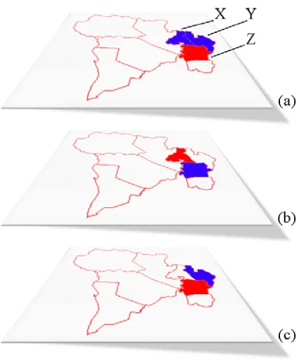
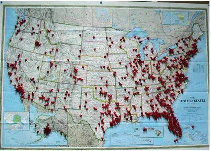
(15) List of Figures 1.1. Example cross-patterning: (a) sexual assault; (b) university locations; (c) overseas visitor population. . . . . . . . . . . . . . . . . . . . . . . . . . . . . . . . .. 2. 1.2. Activities performed for spatial analysis of areal aggregated crime datasets. . . . .. 7. 1.3. Cross-Patterning discovery techniques. . . . . . . . . . . . . . . . . . . . . . . .. 8. 2.1. Example of Layers in a GIS . . . . . . . . . . . . . . . . . . . . . . . . . . . . . 15. 2.2. Geographic Knowledge Discovery . . . . . . . . . . . . . . . . . . . . . . . . . . 17. 2.3. Snow’s Cholera Map (Broad Street Pump circled, with black areas indicating Cholera victims) . . . . . . . . . . . . . . . . . . . . . . . . . . . . . . . . . . . 21. 2.4. Common classification techniques provided by ArcGIS: (a) Raw data; (b) Equal area classification; (c) Equal interval classification; (d) Natural breaks classification; (e) Quantile classification; (f) Standard deviation classification. . . . . . . . . 23. 2.5. Example Co-locations . . . . . . . . . . . . . . . . . . . . . . . . . . . . . . . . 26. 2.6. An example of a traditional pin map.. . . . . . . . . . . . . . . . . . . . . . . . . 29. 2.7. An example of a modern pin map of crime in an area of Houston, Texas.. . . . . . 30. 2.8. An example of a modern pin map of fires in Victoria, Australia. . . . . . . . . . . 31. 2.9. COPLINK display of criminal activity. . . . . . . . . . . . . . . . . . . . . . . . 32. 2.10. COPLINK Spatio-Temporal Visualizer showing Bank Robberies (September-December, 2001). . . . . . . . . . . . . . . . . . . . . . . . . . . . . . . . . . . . . . . . . . 33. 3.1. Study region: (a) Map of Australia; (b) Map of the greater Brisbane area. . . . . . 37. 3.2. Study region: Urban suburbs of Brisbane, Australia. . . . . . . . . . . . . . . . . 38. 3.3. A crime taxonomy tree illustrating various crime types in Queensland. . . . . . . . 40. 4.1. The framework of areal categorised geospatial knowledge discovery.. . . . . . . . 45 xiv.

(16) L IST OF F IGURES. 4.2. xv. Area-to-area aggregation: (a) A base map; (b) A target map labelled with corresponding percentages of offences against person over total offences; (c) An overlay of the base map and the target map. . . . . . . . . . . . . . . . . . . . . . 47. 4.3. Categorisation with natural breaks: (a) A base map with national parks; (b) The base map with histograms; (c) A choropleth map by natural breaks with 5 classes.. 48. 4.4. Synthetic datasets for ACMAM: (a-c) Datasets dataset4.1a−c ; (d) Base region. . . 49. 5.1. Example cross-varying: (a) Murder (left) and Reserves (right); (b) Reserves (left) and Hospitals (right). . . . . . . . . . . . . . . . . . . . . . . . . . . . . . . . . . 55. 5.2. Drawback of Pearson’s correlation coefficient with spatial data: (a-c) Datasets dataset5.1a−c . . . . . . . . . . . . . . . . . . . . . . . . . . . . . . . . . . . . . 57. 5.3. Synthetic hexagon dataset I: (a-d) Datasets dataset5.2D−D3 . . . . . . . . . . . . . 59. 5.4. Comparison of Lee’s L and Wartenberg’s I with synthetic hexagon dataset I (dataset5.2D−D3 ). . . . . . . . . . . . . . . . . . . . . . . . . . . . . . . . . . . 60. 5.5. Synthetic hexagon dataset II: (a) Dataset dataset5.3a ; (b) Dataset dataset5.3t . . . 61. 5.6. Synthetic hexagon dataset III: (a-d) Datasets dataset5.4E−E3. . . . . . . . . . . . 62. 5.7. Comparison of Lee’s L and Wartenberg’s I with synthetic hexagon dataset III (dataset5.4). . . . . . . . . . . . . . . . . . . . . . . . . . . . . . . . . . . . . . 63. 5.8. Synthetic hexagon dataset IV: (a-b) Datasets dataset5.5a−b . . . . . . . . . . . . . 64. 5.9. Irregular region dataset: (a-c) Datasets dataset5.6a−c ; (d) Region outline. . . . . . 65. 5.10. Spatial lag of irregular dataset datasets5.6: (a-b) Unmodified weight matrix; (c-d) Modified weight matrix. . . . . . . . . . . . . . . . . . . . . . . . . . . . . 66. 5.11. Synthetic dataset removing clusters: (a-d) Datasets dataset5.7 a−d . . . . . . . . . . 67. 6.1. Example cross-distribution: (a) Rape and Railway Stations; (b) Fraud and College. 71. 6.2. Working principle of our framework: (a-c) Datasets dataset6.1a−c before normalisation; (d) GLS region ordering; (e) Density trace; (f) Density trace with area highlighted. . . . . . . . . . . . . . . . . . . . . . . . . . . . . . . . . . . . 73.

(17) L IST OF F IGURES. 6.3. xvi. Spatially aware region ordering: (a) Base map including centre points; (b) GLS; (c) DFS; (d) BFS; (e) NN-5; (f) Variance of edge lengths.. . . . . . . . . . . . . . 83. 6.4. Density Trace: (a) Two datasets; (b) Subset of all datasets. . . . . . . . . . . . . . 85. 6.5. Region Weighted Locality In-between Polylines. . . . . . . . . . . . . . . . . . . 85. 6.6. A subset of regions from the Brisbane base map with synthetic data: (a-d) Datasets dataset6.2a−d . . . . . . . . . . . . . . . . . . . . . . . . . . . . . . . . . . . . . 88. 6.7. Optimal ordering: (a) GLS; (b) DFS; (c) BFS; (d) NN-5; (e) Optimal order with same starting region. . . . . . . . . . . . . . . . . . . . . . . . . . . . . . . . . . 89. 6.8. Comparison of normalised density dissimilarity of synthetic datasets using various orders. . . . . . . . . . . . . . . . . . . . . . . . . . . . . . . . . . . . . . . 89. 6.9. Synthetic experiment removing clusters: (a-d) Datasets dataset6.3 a−d ; (e) Increasing dissimilarity with respect to number of removed clusters. . . . . . . . . . 91. 6.10. Synthetic experiment removing clusters: (a) Initial dataset dataset6.4 a ; (b) Increasing dissimilarity with respect to number of removed clusters. . . . . . . . . . 92. 6.11. Synthetic experiment with moving clusters: (a-e) Datasets dataset6.5 a−e ; (f) Increasing dissimilarity with respect to number of moved clusters. . . . . . . . . . . 93. 6.12. Synthetic experiment with moving clusters: (a) Initial dataset dataset6.6 a ; (b) Final dataset dataset6.6u ; (c) Increasing dissimilarity with respect to number of moved clusters. . . . . . . . . . . . . . . . . . . . . . . . . . . . . . . . . . . . . 94. 6.13. Generated graph of base map. . . . . . . . . . . . . . . . . . . . . . . . . . . . . 96. 6.14. Synthetic experiment with moving clusters: (a-e) Datasets dataset6.7 a−e . . . . . 97. 6.15. MSTs of synthetic dataset: (a-e) MST of Datasets dataset6.7a−e from Fig. 6.14. . 99. 6.16. Correlations from synthetic dataset dataset6.7 using minimum edge weight and Pearson’s r . . . . . . . . . . . . . . . . . . . . . . . . . . . . . . . . . . . . . . 100. 6.17. Correlations from synthetic dataset dataset6.7 using MST and Pearson’s r . . . . 100. 6.18. Correlations from synthetic dataset dataset6.7 using MST and Jaccard’s J . . . . 101. 6.19. Synthetic experiment with moving clusters: (a) Initial dataset dataset6.8 a ; (b) Final dataset dataset6.8u ; (c) Correlations using MST. . . . . . . . . . . . . . . . 101. 6.20. Synthetic dataset removing clusters: (a-d) Datasets dataset6.9 a−d . . . . . . . . . 107.

(18) L IST OF F IGURES. 6.21. xvii. Correlations from synthetic dataset dataset6.9 using minimum edge weight and Pearson’s r . . . . . . . . . . . . . . . . . . . . . . . . . . . . . . . . . . . . . . 107. 6.22. Correlations from synthetic dataset dataset6.9 using MST and Pearson’s r . . . . 108. 6.23. Correlations from synthetic dataset dataset6.9 using MST and Jaccard’s J . . . . 108. 6.24. Synthetic experiment removing clusters: (a) Initial dataset dataset6.10 a ; (b) Increasing dissimilarity with respect to number of removed clusters. . . . . . . . . . 109. 7.1. Visualisation of synthetic result set 1 - random layout. . . . . . . . . . . . . . . . 114. 7.2. Visualisation of synthetic result set 1 - circular layout. . . . . . . . . . . . . . . . 114. 7.3. Visualisation of synthetic result set 1 - 2D spring layout. . . . . . . . . . . . . . . 115. 7.4. Visualisation of synthetic result set 1 - 3D spring layout. . . . . . . . . . . . . . . 116. 7.5. Visualisation of synthetic result set 2 - random layout. . . . . . . . . . . . . . . . 117. 7.6. Visualisation of synthetic result set 2 - 2D spring layout. . . . . . . . . . . . . . . 118. 7.7. Visualisation of multiple result sets - random layout. . . . . . . . . . . . . . . . . 118. 7.8. Visualisation of multiple result sets - circular layout. . . . . . . . . . . . . . . . . 119. 7.9. Visualisation of multiple result sets - 2D spring layout. . . . . . . . . . . . . . . . 119. 7.10. Visualisation of multiple result sets - 3D spring layout. . . . . . . . . . . . . . . . 120. 7.11. Visualisation of synthetic result set 3 - circular layout. . . . . . . . . . . . . . . . 122. 7.12. Visualisation of synthetic result set 3 - 2D spring layout. . . . . . . . . . . . . . . 123. 8.1. Boolean ACMAM with support and confidence values. . . . . . . . . . . . . . . . 126. 8.2. Boolean ACMAM with support and lift values. . . . . . . . . . . . . . . . . . . . 126. 8.3. Visualisation of Boolean ACMAM - Random layout. . . . . . . . . . . . . . . . . 127. 8.4. Visualisation of Boolean ACMAM - Circle layout. . . . . . . . . . . . . . . . . . 127. 8.5. Visualisation of Boolean ACMAM - 2D spring layout. . . . . . . . . . . . . . . . 128. 8.6. Quantitative ACMAM with support and confidence. . . . . . . . . . . . . . . . . 129. 8.7. Quantitative ACMAM with support and lift. . . . . . . . . . . . . . . . . . . . . . 130. 8.8. Visualisation of Quantitative ACMAM - Random layout. . . . . . . . . . . . . . . 130. 8.9. Visualisation of Quantitative ACMAM - Circle layout. . . . . . . . . . . . . . . . 131. 8.10. Visualisation of Quantitative ACMAM - 2D spring layout. . . . . . . . . . . . . . 132.

(19) L IST OF F IGURES. xviii. 8.11. Number of generated frequent itemsets and rules using boolean ACMAM . . . . . 133. 8.12. Number of generated frequent itemsets and rules using quantitative ACMAM . . . 133. 8.13. Visualisation of top-50 cross-varying patterns.. . . . . . . . . . . . . . . . . . . . 134. 8.14. Visualisation of bottom-50 cross-varying patterns. . . . . . . . . . . . . . . . . . 135. 8.15. Visualisation of selected top-k crime cross-varying patterns. . . . . . . . . . . . . 135. 8.16. Visualisation of Density Tracing top-50 cross-distribution patterns.. . . . . . . . . 136. 8.17. Visualisation of Density Tracing top-50 cross-distribution patterns.. . . . . . . . . 137. 8.18. Visualisation of Density Tracing selected cross-distribution patterns. . . . . . . . . 138. 8.19. Lowering minimum similarity to reduce cross-distribution patterns. . . . . . . . . 138. 8.20. Comparison between GLS, DFS and BFS for kidnapping. . . . . . . . . . . . 139. 8.21. Comparison between weighted and non-weighted regions for reserves.. . . . . 139. 8.22. Visualisation of Graph Mining top-50 cross-distribution patterns. . . . . . . . . . 141. 8.23. Visualisation of Graph Mining bottom-50 cross-distribution patterns. . . . . . . . 141. 8.24. Visualisation of all cross-patterning - Random layout.. . . . . . . . . . . . . . . . 143. 8.25. Visualisation of all cross-patterning - 2D spring layout. . . . . . . . . . . . . . . . 143. 8.26. Visualisation of all cross-patterning - 3D spring layout. . . . . . . . . . . . . . . . 144. 8.27. Visualisation of overlapping cross-patterning - Circle layout. . . . . . . . . . . . . 144. 8.28. Visualisation of overlapping cross-patterning - 2D spring layout. . . . . . . . . . . 145. 8.29. Computational comparison of approaches for discovering cross-patterning. . . . . 146. 8.30. Computational comparison between Density Tracing and Graph based approach for discovering cross-distribution patterns . . . . . . . . . . . . . . . . . . . . . . 146.

(20) C HAPTER 1. Introduction. Intelligent crime data analysis facilitates an improved understanding of the dynamics of criminal activities such as robbery or assault. It aims to discover patterns of criminal behaviour that may assist in the discovery of where, when and why particular crimes are likely to occur. Criminal behaviour is dependent upon situational factors and as such is patterned according to the location of criminogenic environments. Crime will be concentrated around crime opportunities and other environmental features that facilitate criminal activity. These environmental factors may include socio-economic, socio-demographic or geospatial features. Criminals are creatures of habit and tend to have repetitive patterns of behaviour [94]. For example, some studies suggest that one third of convicted burglars admit to returning to the same residence more than once [35]. Law enforcement agencies can be more effective if they have information about perpetrators’ habits and areas they choose to commit crimes. To fully take advantage of this characteristic, crime data analysis techniques must capture connections between places and events based on past crimes. Decreases in storage costs and ease of spatial data collection has meant that the amount of features available for analysis has grown substantially over recent years. Each of these features are represented as a layer, defined as a spatial dataset consisting of one thematic topic. For example one layer may contain suburb aggregates for murder while another layer contains aggregates for arson. To enable crime data analysis, data mining and knowledge discovery techniques have become essential tools to capture connections between many hundreds of these spatial layers.. 1.

(21) 1 I NTRODUCTION. 2. F IGURE 1.1: Example cross-patterning: (a) sexual assault; (b) university locations; (c) overseas visitor population.. The Queensland Police Service (QPS) and Australian Bureau of Statistics (ABS) record crime and census information in areal aggregated datasets due to limited environmental circumstances and ethical issues such as concern for the privacy of individuals. Areal aggregated spatial datasets are region based datasets that have aggregate data values for regions, e.g. a particular suburb may have recorded five assaults. Regions that share a boundary are defined as neighbours. To enable intelligent crime analysis with these areal aggregated datasets, the relationship between many different spatial layers across locations needs to be modelled and quantified. Cross-patterning describes patterns that occur together in some geospatial region across multiple layers. For example, Fig. 1.1 shows three areal aggregated spatial datasets with colour coded aggregate data values (white=1, blue=2, red=3). An example cross-patterning relationship may be that incidents of sexual assault in region X and neighbouring regions Y and Z show cross-patterning with university locations in region X, Z and an overseas visitor population in region Y, Z..

(22) 1 I NTRODUCTION. 3. This thesis focuses on developing a framework for the discovery and visualisation of crosspatterning in areal aggregated spatial datasets. We identify three ways cross-patterning can be modelled; cross-association, cross-varying and cross-distribution. Cross-association patterns ignore the effect of neighbouring regions. For example it would model the relationship between {robbery in region X, schools in region X}. Cross-varying patterns take into consideration the effect of all neighbours in the local region (i.e. all neighbours that share a border with the region). For example it would model the relationship between {robbery in region X, robbery in neighbouring regions of X, schools in region X, schools in neighbouring regions of X}. Cross-distribution patterns consider one neighbouring region and the global distribution of the dataset. For example it would model the relationship between {robbery in region X, robbery in one neighbouring region of X, global distribution of robbery, schools in region X, schools in one neighbouring region of X, global distribution of schools}. We consider three ways to model cross-patterning so as to provide a generic framework that can be used within many disciplines and applications. Tobler’s first law of geography states that ‘everything is related to everything else, but near things are more related than distant things’ [84]. When analysing areal aggregated spatial datasets, this means that neighbours (those that share a boundary) should be considered. This is achieved in our framework by discovering crossvarying patterns (all local neighbours) and cross-distribution patterns (one local neighbour and the global spatial distribution). In some applications, for computational efficiency or when performing non-spatial metadata analysis, neighbouring information may be ignored. In our framework this is achieved by cross-association patterns. In many applications, analysts can benefit from a combination of the three types of crosspatterning. Our framework is able to discover each type and then using a visualisation environment we are able to highlight overlapping patterns. These overlapping patterns indicate that more than one type of cross-patterning has been discovered and may be of particular interest to the user..

(23) 1.1 M OTIVATION. 4. The core objective of this thesis is the development of a framework for the discovery and visualisation of cross-patterning in areal aggregated spatial datasets. We identify and define three ways cross-patterning can be modelled to discover interesting patterns across spatial layers. We also develop a visualisation environment that enables users to easily interpret the resulting cross-patterning. The algorithms we develop for discovering cross-patterning relationships are designed so they can be applied to areal aggregated spatial datasets from a wide variety of disciplines. For example, the framework presented in this thesis can be applied to spatial datasets in disaster management, epidemiology, business intelligence, geology, environmental monitoring, marketing and e-commerce. One of the motivating factors of this thesis is to improve analysis of crime datasets to allow reasoning towards better decision making and as such we provide a case study that shows how these algorithms are suited for such a purpose. The following section highlights the motivation behind this thesis while Section 1.2 provides an overview of our contributions. Section 1.3 outlines the content of this thesis.. 1.1 Motivation The focus of this thesis is on the development of a framework for the discovery and visualisation of interesting patterns across many spatial layers of areal aggregated data. Our specific application of these tools is to assist in providing a deeper understanding of criminal events and behaviour in areal aggregated crime datasets. Therefore it is necessary that we first describe why crime data analysis is a challenging, interesting and important area of study. We then describe how advances in computer storage and spatial data collection pose challenges to crime data analysis that must be overcome. Intelligent crime data analysis is of great importance to a number of people and agencies such as regional planners, politicians, police and residents. Regional planners can use information about environmental features that attract crime to design safer living environments (for example, with good lighting). Politicians can develop policies and laws to help deter criminals and.

(24) 1.1 M OTIVATION. 5. reduce the incidence of crime. Police can use knowledge about criminal patterns to develop preventative crime strategies, and to help catch offenders. While residents can use this information to try to avoid falling victim to crimes. The costs of crime go far beyond economic, which alone in Australia was estimated at nearly AU$36 billion a year in 2005, to include social, political and environmental factors [74]. Therefore, improving our understanding of crime is of benefit to all members of society. The distribution of crime in time and space is non-random. Because criminal behaviour is dependent upon situational factors, crime is patterned according to the location of criminogenic environments. Crime will be concentrated around crime opportunities and other environmental features that facilitate criminal activity. For example, the top three locations for armed robbery in Australia during 2006 in decreasing order were on the street and footpath, from a retail store and from a service station. This is largely due to their perception as easy targets [50]. Also, in Queensland, the highest residential burglary rates were in coastal tourist regions, inner city areas of Brisbane and a band of suburbs south of Brisbane between Ipswitch and Beenleigh [24]. The purpose of crime analysis is to identify and describe crime patterns such as these [94]. Environmental criminology is a branch of criminological theory that can guide crime analysis and crime prevention efforts. The goal of environmental criminology is to understand the various aspects of a criminal event in order to identify patterns of behaviour and environmental factors that create opportunities for crime [13]. Discovering crime and spatial features that exhibit cross-patterning relationships is a key component to environmental criminology and provides insight into the complex nature of criminal behaviour. These resulting patterns may be possible causal factors that warrant further investigation. For example, determining that criminal offences involving receiving stolen property show a cross-patterning relationship to improvised homes and parks could lead to a targeted crime prevention effort by police in those specific areas. Improvised homes and parks may not be the causal factors of receiving stolen property, but their cross-patterning makes the pattern valuable to police and policy makers..

(25) 1.1 M OTIVATION. 6. Crime, socio-demographic information and environmental feature datasets are maintained by different government and civilian agencies. As with traditional databases, the decrease in storage costs and ease of data collection has led to a data rich environment. This growth in data has increased the need to make sense of it. Data mining has therefore gathered significant attention, as it has the capability of providing a better understanding of the information contained within the data. The aim of data mining is to find previously unknown, nontrivial information from data. This process is automated using algorithms that enable the efficient discovery of such information from the data. Crime has a spatial component (where the crime took place) and as such techniques for crime analysis should consider this spatial information. In additional to the location information contained in such datasets, they also contain textual and/or numeric attributes to describe the feature. For example, the street address of a school is recorded along with information such as the number of pupils, teachers and buildings. Due to the greater complexity of spatial data compared to traditional data, previous methods for data mining are generally not suitable for application directly on spatial data [78]. As a result, new data mining techniques to discover information from spatial data have been developed. However, many spatial data mining techniques, such as predictive modelling, spatial clustering and spatial outlier detection, typically focus on a single spatial layer. To enable crime data analysis, techniques that are able to capture connections and relationships between many hundreds of spatial layers from a wide variety of sources are needed. In addition, a framework is needed that can use heterogeneous data types (such as areal aggregated, point and line datasets) from a wide variety of sources (such as police agencies, census agencies, local councils), efficiently mine these datasets for cross-patterning relationships and then present information to the user in a usable fashion. Obtaining useful information from these crime datasets is a non-trivial task due to the high number of datasets to be considered and the high number of possible cross-patterning relationships within these datasets..

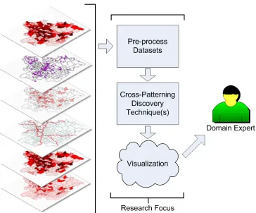
(26) 1.2 C ONTRIBUTIONS. 7. F IGURE 1.2: Activities performed for spatial analysis of areal aggregated crime datasets.. 1.2 Contributions There are a four major outcomes that this thesis achieves. They are to: • Identify and define cross-patterning relationships across multiple areal aggregated spatial datasets; • Develop new techniques to discover and model these cross-patterning relationships; • Develop a visualisation environment to enable users to easily interpret the discovered relationships; and, • Use the developed tools for the analysis of crime datasets along with socio-economic, socio-demographic and geospatial features. As with all data mining tasks, the main goal is to provide an improved understanding of the data in the form of information. Figure 1.2 provides an overview of this; many layers of raw.

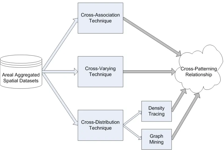
(27) 1.2 C ONTRIBUTIONS. 8. spatial data are available on the left, analysis is performed in the middle section to discover unknown patterns, and then these patterns are presented to the end user in an easy to understand format. This thesis is specifically focused on discovering relationships between different spatial layers across locations. The first part of this work identifies and defines these relationships as cross-patterning relationships. Cross-patterning describes patterns that happen together in some geospatial region across multiple layers. We identify three ways in which cross-patterning can be modelled. These are; cross-association patterns that ignore the effect of neighbouring regions, cross-varying patterns that take into consideration the effect of all local neighbouring regions and cross-distribution patterns that consider one local neighbouring region and the global distribution of the dataset. The second part of this work is to develop techniques to model and quantify each of these types of patterns, as depicted in Figure 1.3.. F IGURE 1.3: Cross-Patterning discovery techniques..

(28) 1.3 T HESIS S TRUCTURE. 9. Cross-association captures the relationship between different spatial layers for each region to allow for the extraction of frequent patterns. We propose an ARM based approach for automating the detection of multivariate cross-associations based on a given areal base map. Crossvarying models patterns using a combination of point-to-point association and spatial dependence. We extend Lee’s bivariate spatial correlation approach [51] to consider areal aggregated datasets containing irregular regions (such as suburbs). Cross-distribution models the spatial distribution of datasets to allow for the discovery of datasets that show similar distribution in similar spatial neighbourhoods. We develop two techniques to discover cross-distribution patterns. Density Tracing incorporates both localised clusters (through the use of context sensitive weighting and clustering) and the global distribution trend. We also investigate an efficient graph based dataset representation that is able to mine a set of datasets for cross-distribution patterns. The visualisation environment developed in the third part of this work serves two purposes. The main purpose is to allow the end user to easily access and interpret cross-patterning information extracted from the datasets. Secondly, it allows for the combination of results from the crossassociation, cross-varying and cross-distribution algorithms, in order to identify those patterns that overlap with each other. These overlapping patterns may be of particular interest and are highlighted to the user. The algorithms developed for discovering cross-patterning relationships are designed so they can be applied to areal aggregated spatial datasets from a wide variety of disciplines. In this thesis we focus on crime analysis and as such we provide a case study that shows how these algorithms are suited for such a purpose.. 1.3 Thesis Structure Following this introduction, we first provide the necessary background information and related work that is required in order to understand the work performed in this thesis. The background begins with an overview of Geographic Information Systems (GIS) and spatial data. Following this, information about geographic knowledge discovery and crime data mining is presented to.

(29) 1.3 T HESIS S TRUCTURE. 10. highlight the need for new algorithms to discover cross-patterning in areal aggregated spatial datasets. Chapter 4 describes the cross-association algorithm, while Chapter 5 details the cross correlation algorithm to model cross-varying. The two algorithms developed to model crossdistribution, Density Tracing and Graph Mining are described in Chapter 6. We describe the visualisation environment and show how the results from cross-association, cross-varying and cross-distribution can be combined in Chapter 7. Chapter 8 presents a case study detailing how cross-patterning can be used for intelligent crime data analysis. We examine each algorithm in detail to analyse crime data from the QPS along with socio-economic, socio-demographic and geospatial features. In this chapter each algorithm’s performance is also compared. Chapter 9 concludes the findings of our research and summarises potential future work that could take place following on from this work..

(30) C HAPTER 2. Related Work. This chapter provides a review of the relevant literature that describes the current landscape of spatial data analysis and crime data analysis. Crime analysis is only possible where data about crimes is available. Therefore the first component to consider is how spatial data is stored and analysed currently using GIS, and the benefits and limitations of such systems for analysis. While these systems are usually able to answer basic locational questions, they are typically unable to provide answers to questions relating to patterns of behaviour. Therefore other techniques need to be investigated to discover such patterns. In developing these techniques it is important to understand that due to the unique features of spatial data, traditional data mining techniques are not always suitable for mining patterns from such data. This has led to the development of new spatial data mining techniques which form part of the process of Geographic Knowledge Discovery (GKD). Specific work has also been conducted in the area of crime data mining which is a subset of spatial data mining. The data we focus on in this thesis is areal aggregated. There are several existing techniques that can be adapted to discover patterns from areal aggregated spatial data. These include hot spot analysis, Spatial Association Rules Mining (SARM) and Co-Location Rules Mining (CLRM). We describe these techniques and provide examples to illustrate their usage. Techniques that are able to discover patterns across multiple layers of areal aggregated data are less well studied and are the focus of this thesis. Once relationships within the datasets have been found, the resulting patterns need to be investigated by an analyst for useful information. Due to the size and complexity of spatial data, many 11.

(31) 2.1 OVERVIEW. 12. of these techniques discover a large number of complex patterns. Therefore the next challenge is to provide the most important, useful and relevant information to the analysts. Visualisation is a clear and effective technique for communicating these results. This chapter outlines related work that has contributed and led to the development of the techniques introduced in this thesis, which enable crime analysts to gain greater knowledge and understanding about criminal patterns of behaviour.. 2.1 Overview This section introduces the GIS which is the primary storage location for most geographic and spatial data. While GISs have been around since the early 1960s [71], they were not widely available until the early 1980s. This was helped along by the increasing adoption of Personal Computers such as that by IBM in 1982. Improvements in technology eventually lead to a number of GIS vendors producing commercial GIS products, such as those released by the Environmental Systems Research Institute (ESRI) and MapInfo. Microsoft has also recently started to provide some spatial tools as part of it’s SQL Server 2008 suite at a more affordable price than some of the dedicated GIS vendors, allowing more users to store and use spatial data. In more recent years, increasing amounts of spatial data are becoming available due to developments in both collection and storage technology. For example, improvements in the performance of telescopes have enabled the Sloan Digital Sky Survey (SDSS) [7] to collect data and map a large number of galaxies, quasars and stars. On a smaller scale, Google is encouraging organisations and individuals to provide and access spatial information through their Google Maps technology, which is widely available to the public [33]. Different types of spatial data are also increasingly being captured and in some cases being made publicly available either directly or through applications that are built from them [6, 29, 85]. Governments and organisations are coming to realise the benefits of spatial mapping where both types of enterprises can use spatial information for the provision of services and for planning..

(32) 2.1 OVERVIEW. 13. As the size and types of spatial data is increasing, the ability to analyse and understand it is a growing challenge. Additionally, spatial data contains some complexities over traditional transactional data that must be taken into account when developing pattern discovery techniques. In this section we introduce GISs, their benefits and limitations and then describe the complexities of the spatial data that they store. A more detailed description of the crime data used in this thesis is provided in Chapter 3.. 2.1.1 Geographic Information Systems Most spatial data is stored in a GIS. A GIS is defined as a tool for the manipulation of geographic data [11]. The GIS performs a great diversity of functions; some of which include compilation, verification, storage, retrieval, manipulation, update and visualisation of geographic data. The adoption and storage of data into GISs has allowed users to find answers to spatially-related queries. Some such queries may be, ‘What are the names of all customers who live within 10km of my store?’, or ‘What are all the crimes that have occurred within a 5km radius of my service station?’. Another example may be a query from a mobile device user who may ask ‘Where is the nearest Automatic Teller Machine (ATM)?’. The latter example is already being performed through the use of a GIS by Mastercard [57]. However, while the advances in spatial GISs are significant and important, realising the full value of spatial data is not yet complete. Growth in the use of such systems has led to an increase in the storage of spatial data. As with traditional databases, the decrease in storage costs and ease of data collection has meant that gathering useful and interesting spatial information is a difficult but important task. Most GISs, without the help from spatial data mining techniques, are not able to mine spatial data to find interesting and previously unknown information. Some examples of such information are ‘What services are frequently requested together from a mobile device?’ or ‘Around which spatial features is crime likely to occur near?’..

(33) 2.1 OVERVIEW. 14. One of the reasons spatial information discovery is challenging is that GISs often store multiple layers of spatial data. Each layer represents a different feature set. Figure 2.1 illustrates some examples of layers that can be stored in a GIS. The layers in this example include census information along with locations of crimes, parks, schools and train stations. Being able to find relationships in the data between layers is important in understanding patterns of criminal behaviour. In this example, we may be able to find relationships between the locations of particular crimes and the locations of parks or schools. Layers can also be at different granularities [59] and consist of different spatial data types (lines, points, grids, regions) which can also make pattern discovery more challenging. Each layer can also hold additional information about the data points or regions captured. For example, crime data can indicate the type and time of a particular crime incident, and park data could include the size or activity level of a park. Spatial data mining as described in the subsequent sections, is able to provide a solution to this problem. It can be used to discover patterns from multiple layers of spatial data, so that inferences can be drawn about relationships between the location of particular events and other features.. 2.1.2 Spatial Data Spatial data is data that contains thematic and geographic attributes. For example, the thematic attribute could be the type of crime committed (such as arson) or the land feature (such as a park). The geographic attribute is the location of the thematic attribute, that is, the location where the crime occurred, or the location of the park. With an increasing amount of spatial data available, there has been a growing need to mine information about the types of patterns that are prevalent in the data. However, this is a difficult task as there are many features of spatial data that must be considered. One of the most cited differences between spatial and non-spatial data is that observations are usually not independent [36, 69] and identically distributed (i.i.d.). Statistical independence.

(34) 2.1 OVERVIEW. 15. F IGURE 2.1: Example of Layers in a GIS. means that the occurrence of one event has no effect on the likelihood of the occurrence of another event. An example of how spatial data is not independent is that weather conditions in one region is influenced by weather conditions in neighbouring regions. Identical distribution means that each observation should have the same probability distribution as any other observation. However in the case of spatial data, the probability of certain values occurring is influenced by the values of neighbouring observations. As stated in Chapter 1, Tobler’s first law of geography states that ‘everything is related to everything else, but near things are more related than distant things’ [84]. The term ‘spatial autocorrelation’ is also often used to describe this phenomenon. Spatial autocorrelation is.

(35) 2.2 S PATIAL DATA M INING AND G EOGRAPHIC K NOWLEDGE D ISCOVERY. 16. defined by Goodchild [31] as “the degree to which objects or activities at some place on the Earth’s surface are similar to objects or activities nearby”. Another consideration when mining spatial data is that there are at least two types of information for any given spatial data point [31]. That is, their location, which may be specified using co-ordinates for example, and their attributes which are the variable values taken for that location, such as the number of crimes committed. Such features mean that traditional approaches to mining transactional data are not easily applied to spatial data. In order to handle such data, spatial data mining techniques need to be developed. Some such techniques are highlighted in Section 2.2.. 2.2 Spatial Data Mining and Geographic Knowledge Discovery Geographic Data Mining (GDM) is a component of GKD. GKD is the process of extracting information and knowledge from massive geo-referenced databases [62]. GDM involves the use of computational techniques and tools to discover patterns that are distributed over geographic space and time [62]. It is also sometimes referred to as spatial data mining within the data mining community [47, 76]. The GKD process is shown in Figure 2.2. The first step is to extract the raw spatial data from a spatial data store. The extracted data may not be in the desired form for GDM, therefore some preprocessing may be required. As with data in traditional databases, this data may contain some inconsistencies, such as missing data that should be dealt with prior to the GDM process. The layers that are to be mined should also be specified and those layers extracted. As spatial data layers may be stored in different granularities, any aggregations should also be made to this data to simplify GDM where necessary. Once the preprocessing is complete, GDM algorithms may be run to discover patterns from the data. Some examples of GDM techniques are outlined in Section 2.3. Once patterns are.

(36) 2.2 S PATIAL DATA M INING AND G EOGRAPHIC K NOWLEDGE D ISCOVERY. 17. F IGURE 2.2: Geographic Knowledge Discovery. retrieved, they are often returned in plain text format, or other formats that are difficult to interpret. Therefore a postprocessing step must take place to attempt to transform the data into more useful information. This step involves filtering out any uninteresting patterns and providing a graphical visualisation to the end user expert. The final stage is for the expert to investigate possible relationships further and potentially gain further knowledge about the discovered patterns. Geoinformation and spatial data have unique characteristics that some data mining techniques do not take into consideration [28, 69]. Openshaw [69] defines GDM as ‘a special type of data mining that seeks to perform similar generic functions as conventional data mining tools, but modified to take into account the special features of geoinformation, the rather different styles and needs of analysis and modelling relevant to the world of GIS, and peculiar nature of geographical explanation.’ Therefore, in order to detect geographically interesting patterns, GDM techniques must consider the unique features of geographic data in order to find potentially interesting geographical patterns. The discovered patterns can be either descriptive or prescriptive. Descriptive pattern mining techniques summarise and characterise the data. Prescriptive pattern mining techniques attempt to predict patterns by drawing inferences from the data. Geographic Data Mining, as a quantitative study of georeferenced phenomena, explicitly focuses on the geospatial features of the data such as location, distance, interaction and geospatial arrangement [5, 10]..

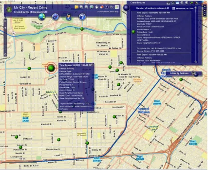
(37) 2.2 S PATIAL DATA M INING AND G EOGRAPHIC K NOWLEDGE D ISCOVERY. 18. 2.2.1 Crime Data Mining. Crime data mining has gained significant attention among academics over the past decade as terrorist attacks have become more widespread and as data mining techniques have become more mature. Crime data mining builds on traditional data mining techniques and applies them to different types of crimes [17, 18]. Most research in crime data mining has focused on the application side. Dedicated novel crime data mining methods have been relatively less studied. Although several efforts have been made to develop variants of dedicated crime data mining techniques, they are task-specific and still lack a unifying crime data mining framework [17]. For the analysis of crime data, data mining techniques have been applied by the US Federal Bureau of Investigation (FBI) as a part of the investigation of the Oklahoma City bombing (Unabomber case), and many lower-profile crimes [12]. Data mining has also been used by the US Treasury Department to hunt for suspicious patterns in international funds transfer records; patterns that may indicate money laundering or fraud [12]. Examples also include the Health Insurance Commission of Australia using data mining to investigate fraud within the Medicare system [42] and National Roads and Motorists’ Association (NRMA) Insurance Ltd [91]. However, in the above examples, the techniques have been limited to the thematic attributeoriented side of the data, while often ignoring the spatial and temporal attributes. The where and when are crucial for patterns of crime. Recent progress towards developing GIS for crime analysis emphasises the relevance that georeference has to understand patterns in crime [44]. In a limited exploratory approach, systems have been developed to geographically visualise patterns of vehicle crime, domestic burglaries, drug-related crime and public disorder in inner city areas [68], and violent crimes in Brisbane [64, 65]. The COPLINK project [17, 40, 41] developed by the University of Arizona Artificial Intelligence Lab in collaboration with the Tucson Police Department is the most comprehensive crime data mining suite. It consists of several different modules conducting various.

(38) 2.3 S PATIAL PATTERN M INING T ECHNIQUES. 19. crime data mining functions including link analysis visualisation, incident analysis though clustering, visualisation through geospatial mappings, and geospatial/temporal analysis. Although this suite provides a list of comprehensive data mining techniques, there are several limitations associated with it. Firstly, it mainly focuses on link analysis to find strong associations in organised crimes. Incident analysis is based on point data not areal aggregated data. Socio-demographic data is not properly considered in the geospatial domain, and the level of detail in data significantly differs from the level of detail in areal aggregated crime data available from the QPS.. 2.3 Spatial Pattern Mining Techniques. The most common techniques used to extract patterns from spatial data include hot spot analysis, SARM and CLRM. Hot spot analysis is the discovery of areas with particularly high levels of the occurrence of some spatial feature. A crime hot spot can be generally defined as ‘an area containing dense clusters of criminal incidents’ [3]. It is a descriptive mining tool that is able to summarise and characterise the data. Hot spot analysis can is also one way of performing deviation detection, and can also be used as a type of trend detection. Spatial association rules and co-location rules are both predictive pattern mining tools that can draw inferences from the data for predictions. A spatial association rule is a rule of the form A → B, where A and/or B are a set of non-spatial and sometimes spatial predicates. For example, a strong spatial association rule may be that 90% of sexual assaults may occur in parks. Co-location rules are defined as non-spatial items that frequently occur together over space [79]. These techniques are discussed in further detail in the following subsections..

(39) 2.3 S PATIAL PATTERN M INING T ECHNIQUES. 20. 2.3.1 Hot Spot Analysis. Hot spot analysis is the discovery of areas with particularly high levels of the occurrence of some spatial feature. For example, there may be a particularly high rate of illness or crime in one particular area. One of the earliest and most commonly cited hot spot analysis was performed by John Snow in Soho, England in response to a Cholera outbreak during 1854 [80]. By plotting the location of cholera victims on a map of London city shown in Figure 2.3 he showed that many of the victims were situated around a particular water pump location on Broad Street. The discovery of this cholera ‘hot spot’ led authorities to remove the handle from the water pump. The availability of spatial data and the introduction of storage systems such as GISs has enabled hot spot analysis to be performed on much larger sets of spatial data, and on a variety of different types of data. In crime analysis, the use of hot spots to determine policing and crime prevention strategies has grown over recent years [23, 44, 56, 64, 72]. Crime hot spots have appealed to both crime prevention practitioners and police managers [72]. Current GISs such as ArcGIS provide a limited range of data classification methods for hot spot analysis such as natural breaks, quantiles, equal area, equal interval and standard deviations [27]. Figure 2.4 shows various classification methods available within ArcGIS for the crime dataset, Fraud by Cheque, from Brisbane, Australia. Natural breaks (Figure 2.4(d)) divide the data by identifying natural groupings and ‘break points’ in the data that best group similarities within a class and maximise differences between classes. That is, boundaries are set where there are large jumps between neighbouring values. This method is best used when there is uneven distribution of values. In quantile classification (Figure 2.4(e)), the number of values is the same in each class. This is achieved by dividing the range of possible values into unequal-sized intervals. Classes at the extremes have a wider interval range. Therefore this method is generally used to highlight variations in the middle-values of the distributions..

(40) 2.3 S PATIAL PATTERN M INING T ECHNIQUES. 21. F IGURE 2.3: Snow’s Cholera Map (Broad Street Pump circled, with black areas indicating Cholera victims). The equal interval technique (Figure 2.4(c)) is similar to quantile classification, except that interval ranges are equal for each class. As there are usually less values at the extremes, this technique is generally used to highlight changes in the extreme range of values. Equal area classification (Figure 2.4(b)), also known as Geometrical Interval classification, was designed primarily for use with continuous data. Breaks between classes are based on class intervals that have a geometrical series. A geometric series is created by multiplying all the values in the series by a constant coefficient..

(41) 2.3 S PATIAL PATTERN M INING T ECHNIQUES. 22. The standard deviation classification (Figure 2.4(f)) method shows how much an attribute value deviates from the mean. It places class breaks above and below the mean value at intervals of 1, 0.5, or 0.25 standard deviations. The correct choice of classification method has a great impact on generated hot spots, and thus any reasoning based on these hot spots. Choosing the ‘best’ classification method is heavily dependent on the user’s domain knowledge and even then may require a number of iterations to determine the most suitable method. In data-rich environments, these iterations are timeconsuming and expensive. Most importantly, the boundaries of the base map dominate shapes of crime hot spots and we are not able to find data-oriented natural shapes of crime hot spots with the current techniques available in GISs. Thus, subsequent reasoning about hot spots can be misleading. Several approaches have been made to overcome these inherent limitations of GISs and to identify data-oriented shapes of crime hot spots in the geographical data mining community [23, 56, 64, 72]. These approaches identify base-map-free hot spots based on various clustering criteria. However, relatively little research has been conducted on postclustering and reasoning about crime hot spots for answers to questions such as “why are they there?”. Estivill-Castro and Murray [64] present a partitioning clustering algorithm using a k-medoid type optimisation function. The algorithm uses hill-climbing heuristics to efficiently allow the exploratory analysis of large spatial datasets. The novel idea of stopping these heuristics early is analysed and shown to offer large computational savings while keeping the quality of the clustering high. They show that clustering in respect to a given feature set (such as schools and parks) allows positive associations to be discovered. The downside to their approach is that the clustering algorithm only produces single level clusters and uses k-partitioning clustering. It is known that criminal activities are inherently hierarchical and the number of clusters is unknown [52, 56]. Choosing the best value for k is labourious and non-trivial. Lee and Estivill-Castro [53] present a framework for mining interesting associative patterns in complex crime datasets. They use clustering to identify hot spots, transform them into polygons, and then find possible associative relations with ARM. Their framework considers layers.

(42) 2.3 S PATIAL PATTERN M INING T ECHNIQUES. 23. (a). (b). (c). (d). (e). (f). F IGURE 2.4: Common classification techniques provided by ArcGIS: (a) Raw data; (b) Equal area classification; (c) Equal interval classification; (d) Natural breaks classification; (e) Quantile classification; (f) Standard deviation classification.. of different spatial features and how they impact on each other. The performance of the framework is heavily dependent on the clustering technique and the boundary extraction technique used. The major drawback to this technique is that it uses single-level clustering which does not fully reveal the true structure of complex crime data. A similar framework using hierarchical Short-Long clustering and Region Connection Calculus (RCC) is proposed by Lee and Williams [54]. They use cluster boundary extraction and the resulting polygons to detect relationships between multi-level clusters and to suggest their.

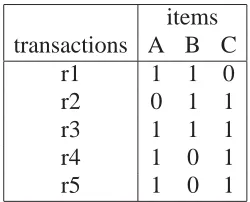
(43) 2.3 S PATIAL PATTERN M INING T ECHNIQUES. 24. positive associations. For massive crime datasets, the computational burden of computing and extracting cluster boundaries limits the usability of both of these techniques. Although there exist a number of techniques available to conduct hot spot analysis, most of these techniques focus on point data. In this thesis we focus on discovering patterns from areal aggregated data.. 2.3.2 Spatial Association Rules Mining Traditional ARM [1, 2, 37, 43] has been a powerful tool for discovering positive associations among a set I = {I1 , I2 , . . . , In } of items in a transactional database D. Here, each transaction T ∈ D is a subset of I. An association rule is an expression in the form of X ⇒ Y (c%), X ∈ I, Y ∈ I, and X ∩ Y = ∅ where X is called antecedent and Y is called consequent. It is interpreted as “c% of transactions in D that satisfy X also satisfy Y ”. Typically, support and confidence are two measures of a rule’s interestingness. Support ensuring statistical significance is the probability that X and Y exist in a transaction T ∈ D. Confidence indicating the rule’s strength is the probability that Y exists in a transaction T given that T contains X. That is, support is an estimate for P rob(X ∪ Y ) and confidence is an estimate for P rob(Y |X). Two user defined thresholds, minimum support and minimum confidence, are used for pruning rules to find only interesting rules. Itemsets satisfying the required minimum support constraint are named frequent while rules satisfying the two thresholds are called strong. Another measure of a rules interestingness is lift [90]. The lift value is given by the ratio of confidence to expected confidence, where the expected confidence is the number of transactions that include the consequent divided by the total number of transactions. Lift indicates the increase in probability of X given Y . Support, confidence and lift are used to filter out uninteresting association rules that are less probable, and thus potentially provide analysts with previously unknown but useful strong association rules that can assist with decision making..

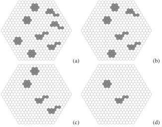
(44) 2.3 S PATIAL PATTERN M INING T ECHNIQUES. 25. Mennis [61] applied traditional ARM to socioeconomic and land cover change analysis. It ignores the spatial dimension and simply converts the spatial database to relational tables to which traditional ARM can be applied. Typically, ARM has been applied to geospatial data in two different ways. This is parallel to the fact that there are two popular views of geographical space in a GIS: vector and raster. The vector view regards geographical space as a set of objects while the raster view sees it as a set of locations. Spatial Association Rules Mining (SARM) [48] is similar to the raster view in the sense that it tessellates a study region S into discrete groups based on spatial or aspatial predicates derived from concept hierarchies. For instance, a spatial predicate close_to(α, β) divides S into two groups, locations close to β and those not. So, close_to(α, β) can be either true or false depending on α’s closeness to β. A spatial association rule is a rule that consists of a set of predicates in which at least one spatial predicate is involved. For instance, is_a(α, house) ∧ close_to(α, beach) ⇒ is_expensive(α). Although this approach efficiently mines complex geospatial datasets, it has several drawbacks. It is not directly applicable to datasets in which transactions can be infinite or indefinite. That is, situations where the traditional interesting measures can not be directly measured. Also, a great degree of human involvement is required to find association rules. In this approach, the predefined concept hierarchy drives the human-oriented rule discovery which does not comply with exploratory data analysis and the principle to “let the data speak for themselves” [34, 68].. 2.3.3 Co-location Rules Mining Co-Location Rule Mining [79] discovers a subset of features given a set of point features frequently located together in a geographic space. An example of this is shown in Figure 2.5, where green circles and red squares are frequently located together. These shapes could represent any two items in space. For example these points could indicate the co-location of public recreation areas and theft, chemical storage facilities and cancer or puma and deer. It extends traditional ARM by providing a transaction free approach of mining co-location rules, using the concept of neighbourhoods without having to define a reference feature. This.

No results found