Numerical study of stream-function formulation
governing flows in multiply-connected domains by
integrated RBFs and Cartesian grids
K. Le-Cao
1, N. Mai-Duy
1∗, C.-D. Tran
1,2and T. Tran-Cong
1 1Computational Engineering and Science Research Centre
Faculty of Engineering and Surveying,
The University of Southern Queensland, Toowoomba, QLD 4350, Australia
2
CSIRO, Geelong,VIC 3216, Australia
Submitted to
Computers & Fluids, 31-March-2010; revised,
3-September-2010
AbstractThis paper describes a new numerical procedure, based on point
colloca-tion, integrated multiquadric functions and Cartesian grids, for the discretisation of
the stream-function formulation for flows of a Newtonian fluid in multiply-connected
domains. Three particular issues, namely (i) the derivation of the stream-function
values on separate boundaries, (ii) the implementation of cross derivatives in
irreg-ular regions, and (iii) the treatment of double boundary conditions, are studied in
the context of Cartesian grids and approximants based on integrated multiquadric
functions in one dimension. Several test problems, i.e. steady flows between a
rotating circular cylinder and a fixed square cylinder and also between eccentric
cylinders maintained at different temperatures, are investigated. Results obtained
are compared well with numerical data available in the literature.
Keywords: Stream-function formulation; multiply-connected domain; integrated
ra-dial basis function network; Cartesian grid
1
Introduction
The motion of a Newtonian fluid is governed by the Navier-Stokes equations which
can be written in terms of different dependent variables, including the velocity
-pressure formulation, the function - vorticity formulation and the
stream-function formulation. The velocity - pressure formulation is able to work for
two-and three-dimension flows in a similar manner. One main concern is that there are
no explicit transport equation and boundary conditions for the pressure variable.
The resultant algebraic system could be solved iteratively where the pressure value
is corrected using the continuity equation. For two-dimensional (2D) problems, by
two (stream-function and vorticity) and only one (stream-function). However, the
last two formulations have some drawbacks. Special attention should be given to
the handling of the vorticity boundary condition for the stream-function - vorticity
formulation and the double boundary conditions as well as high-order derivatives
including the cross ones for the stream-function formulation. Furthermore, the
pres-sure field needs be computed after solving the governing equations, which is generally
regarded as a complicated process. In the case of multiply-connected domains, an
added difficulty is that the stream-function variable generally has different values,
which are unknown, on separate boundaries. It is noted that advantages of the
stream-function - vorticity formulation presented above are restricted to 2D
prob-lems.
The governing differential equations can be transformed into sets of algebraic
equa-tions by means of discretisation. To support the approximaequa-tions, the problem
do-main needs be represented by a set of finite elements, a Cartesian grid or a
collec-tion of discrete points. For problems with complicated geometries such as flows in
multiply-connected domains, it has been recognised that the task of dividing the
spa-tial domain into a number of finite elements can be the most time-consuming part of
the solution process. Generating a Cartesian grid or a set of discrete points is clearly
much more economical. Over the last twenty years, radial-basis-function networks
(RBFNs) have been developed to solve different types of differential problems
en-countered in applied mathematics, science and engineering (e.g. [1,2,3,4,5,6,7,8,9]).
These approximators can work well with gridded and scattered points. As shown in
[10, 11, 12], there is the relation between the RBF collocation method and the finite
difference method (FDM). For 1D approximations, the standard RBF interpolant
converges to the Lagrange interpolating polynomial as the RBF width goes to
in-finity, which means that all classical FD formulas can be recovered by the limiting
clear due to the fact that multivariate polynomial interpolations are not well-posed.
In [4,5,6,7,8], the RBF approximations are constructed using integration (integrated
RBFNs (IRBFNs)) rather than the usual differentiation. This approach has the
abil-ity to overcome the problem of reduced convergence rates caused by differentiation
and to provide effective ways to implement derivative boundary values. IRBFNs
have been developed for the simulation of flows in simply-connected domains
gov-erned by the stream-function formulation and the stream-function - vorticity
formu-lation (e.g. [6]) as well as natural convection in regions between concentric cylinders
governed by the stream-function - vorticity formulation (symmetrical flows) (e.g.
[4]).
This study is concerned with the simulation of unsymmetrical flows of a
Newto-nian fluid in multiply-connected domains using the stream-function formulation,
Cartesian grids and 1D-IRBFNs. Unlike the symmetrical case, the stream-function
variable has different values on separate boundaries. These values can be found
using the single-value condition for the pressure, whose implementations are known
to be difficult (e.g. [13]). Further difficulties include the implementation of cross
derivatives in regions bounded by irregular surfaces as the boundary points do not
generally coincide with the grid nodes. New treatments for these difficulties and
their 1D-IRBF-based implementations are the focal point of this study.
An outline of the paper is as follows. The stream-function formulation and
1D-IRBFNs are briefly reviewed in Section 2 and Section 3, respectively. The proposed
procedure is described in Section 4 and then numerically verified through the
simu-lation of steady flows between a rotating circular cylinder and a fixed square cylinder
and also between eccentric cylinders maintained at different temperatures in Section
2
Governing equations
Consider the stream-function formulation. The non-dimensional basic equations
for natural convection under the Boussinesq approximation in the Cartesian x−y
coordinate system can be written as (e.g. [14])
∂ ∂t
∂2ψ
∂x2 +
∂2ψ
∂y2
+∂ψ
∂y
∂3ψ
∂x3 +
∂3ψ
∂x∂y2
− ∂ψ
∂x
∂3ψ
∂x2∂y +
∂3ψ
∂y3 = r P r Ra
∂4ψ
∂x4 + 2
∂4ψ
∂x2∂y2 +
∂4ψ
∂y4
−∂T
∂x, (1)
∂T ∂t +u
∂T ∂x +v
∂T ∂y = 1 √ RaP r
∂2T ∂x2 +
∂2T ∂y2
, (2)
whereψ is the stream function,T the temperature,t the time,u and v the velocity components, andP randRathe Prandtl and Rayleigh numbers defined asP r=ν/α
and Ra = βg∆T L3/αν, respectively, in which ν is the kinematic viscosity, α the
thermal diffusivity, β the thermal expansion coefficient and g the gravity. In this dimensionless scheme, L, ∆T (temperature difference), U =√gLβ∆T and (L/U), are taken as scale factors for length, temperature, velocity and time, respectively. It
is noted that the velocity scale is chosen here in a way in which the buoyancy and
inertial forces are balanced (e.g. [14]).
For iso-thermal flows, the non-dimensional basic equations reduce to
∂ ∂t
∂2ψ
∂x2 +
∂2ψ
∂y2
+∂ψ
∂y
∂3ψ
∂x3 +
∂3ψ
∂x∂y2
−∂ψ
∂x
∂3ψ
∂x2∂y +
∂3ψ
∂y3 = 1 Re
∂4ψ ∂x4 + 2
∂4ψ ∂x2∂y2 +
∂4ψ ∂y4
, (3)
The velocity components are defined in terms of the stream function as
u= ∂ψ
∂y, (4)
v =−∂ψ
∂x. (5)
The given velocity boundary conditions for u and v can be transformed into two boundary conditions on the stream function and its normal derivative
ψ =γ, (6)
∂ψ
∂n =ξ, (7)
wheren is the direction normal to the boundary, and γ and ξ prescribed functions. For the case of fixed concentric cylinders, non-slip boundary conditions usually lead
to γ = 0 and ξ = 0 at walls. For the case of rotating cylinders and eccentric cylinders, because of the existence of a global circulation flow, the stream-function
values on the inner and outer cylinder walls cannot be the same.
3
Brief review of 1D-integrated RBFNs
In contrast to the traditional/direct/differential approach, where a functionf is ap-proximated by an RBFN, followed by successive differentiations to obtain
approxi-mate expressions for its derivatives, the indirect/integral approach uses integration
to construct the RBF approximations (e.g. [7,8]). A highest-order derivative of f
derivatives and the function itself are then obtained through integration
dpf(x)
dxp = m
X
i=1
wigi(x) = m
X
i=1
wiI( p)
i (x), (8)
dp−1f(x)
dxp−1 =
m
X
i=1
wiI( p−1)
i (x) +c1, (9)
dp−2f(x)
dxp−2 =
m
X
i=1
wiI
(p−2)
i (x) +c1x+c2, (10)
· · · ·
df(x)
dx =
m
X
i=1
wiIi(1)(x) +c1
xp−2
(p−2)! +c2
xp−3
(p−3)! +· · ·+cp−2x+cp−1, (11)
f(x) =
m
X
i=1
wiIi(0)(x) +c1
xp−1
(p−1)! +c2
xp−2
(p−2)! +· · ·+cp−1x+cp, (12)
where {gi(x)}mi=1 ≡
n
Ii(p)(x)om
i=1 is the set of RBFs, m the number of RBFs,
(c1, c2,· · · , cp) the constants of integration and I( p−1)
i (x) =
R
Ii(p)(x)dx, I(p−2)
i (x) =
R
I(p−1)
i (x)dx,· · ·, I
(0)
i (x) =
R
Ii(1)(x)dx. Numerical results (e.g. [7]) have shown that the integral approach significantly improves the quality of the approximation
of derivative functions over conventional differential approaches. The IRBF-based
approximation scheme is said to be of pth-order, denoted by IRBFN-p, if the p th-order derivative is taken as the staring point.
The present technique implements the multiquadric (MQ) function whose form is
gi(x) =
q
(x−ci)2+a2i, (13)
where ci and ai are, respectively, the centre and the width of the ith MQ basis
4
Proposed numerical procedure
Calculations for unsymmetrical flows in multiply-connected domains are carried out
on Cartesian grids. Grid nodes inside the domain of interest are taken to be interior
nodes. Boundary points are generated by the intersection of the grid lines and
boundaries. Boundary nodes are thus comprised of two sets of points. The first set
is generated by the x−grid lines; the other by the y−grid lines.
1D-IRBFNs of orders 4 and 2 are employed on the grid lines to represent the
stream-function and temperature variables, respectively. The governing differential
equa-tions, which involve high-order and cross derivatives, are discretised by means of
point collocation. Emphasis is placed on the following issues: (i) the implementation
of cross derivatives in irregular regions, (ii) the derivation of the stream-function
val-ues on separate boundaries, and (iii) the treatment of double boundary conditions.
Formulas are derived in terms of Cartesian coordinates and they are implemented
with 1D-IRBFNs.
It is noted that conventional RBF methods are global and lead to full matrices.
Unlike conventional methods, at a grid node, the proposed method only uses RBF
centres on the two associated grid lines rather than the whole set of RBF centres to
construct the approximations at that point. The present method thus possesses some
local approximation properties. In comparison with conventional RBF methods,
relatively-large numbers of nodes can be employed here. However, the resultant
system matrix is still not as sparse as those produced by finite-difference methods.
The present technique needs be combined with domain decompositions for handling
4.1
Boundary values for stream function
Since there is no flow in the direction normal to a solid boundary, the stream function
is constant at a wall. The stream-function variable has different values on different
walls. The value of ψ on the outer wall is simply set to zero, while the values of ψ
on inner walls are considered as unknowns. Consider an inner wall. The associated
unknown there cannot be determined from the governing equation; an independent
equation/integral condition is needed. To find the value ofψ on the wall, Lewis [15] suggested using the condition that the pressure is a single-valued function (there
is only one value of pressure at a point). This condition can be mathematically
described as
I
Γ
∂p ∂sds=
I
Γ∇
p·d~s= 0, (14) wherepis the pressure,sthe arc length, dsthe length of an infinitesimal part of the boundary Γ. It should be pointed out that Γ can be any closed path. In the present
work, the inner cylinder boundary is taken to be Γ . The pressure gradient∇p can be obtained from the momentum equations. The reader is referred to, for example,
([15, 16, 17]) for further details. In the Cartesian coordinate system, Equation (14)
becomes
I
∂p ∂xdx+
I
∂p
∂ydy = 0. (15)
From the primitive variable formulation, we have
∂p ∂x =
1
Re
∂2u
∂x2 +
∂2u
∂y2
−
u∂u ∂x +v
∂u ∂y , (16) ∂p ∂y = 1 Re
∂2v
∂x2 +
∂2v
∂y2
−
u∂v ∂x +v
∂v ∂y
Substituting (16) and (17) into (15) and then making use of (4) and (5) lead to
I
∂3ψ
∂2x∂ydx+
I
∂3ψ
∂3ydx−Re
I
∂ψ ∂y
∂2ψ
∂x∂ydx+Re
I
∂ψ ∂x
∂2ψ
∂y2dx−
I ∂3ψ
∂3xdy−
I ∂3ψ
∂2y∂xdy+Re
I ∂ψ
∂y ∂2ψ
∂x2dy−Re
I ∂ψ
∂x ∂2ψ
∂y∂xdy= 0. (18)
In the case of a fixed cylinder, the convection term vanishes on its wall. Equation
(18) thus reduces to
I ∂3ψ
∂2x∂ydx+
I ∂3ψ
∂3ydx−
I ∂3ψ
∂3xdy−
I ∂3ψ
∂2y∂xdy= 0. (19)
By expressing integrals in (18)/(19) in terms of the values ofψat the interior points, the resultant equation can be used as an extra equation to determine the value of
ψ on the wall.
4.2
Cross derivatives
In the present formulations, the governing equations and the single-valued pressure
condition involve cross derivatives, namely∂4ψ/∂2x∂2y,∂3ψ/∂2x∂y, and∂3ψ/∂x∂y2.
As mentioned earlier, the IRBF approximations are constructed on the grid lines.
It is necessary to transform the computation of these mixed derivatives to that of
pure derivatives. This can be achieved through the following relations
∂4ψ
∂2x∂2y =
1 2 ∂2 ∂x2
∂2ψ
∂y2 + ∂ 2 ∂y2
∂2ψ
∂x2
, (20)
∂3ψ
∂2x∂y =
∂2 ∂x2 ∂ψ ∂y , (21)
∂3ψ
∂x∂y2 =
In (20)-(22), there are two terms, namely ∂2(∂2ψ/∂y2)/∂x2 and ∂2(∂ψ/∂y)/∂x2,
to be evaluated on the x−grid lines and two terms, namely ∂2(∂2ψ/∂x2)/∂y2 and
∂2(∂ψ/∂x)/∂y2, to be evaluated on the y−grid lines.
Consider anx−grid line. To carry out the approximation of ∂2(∂2ψ/∂y2)/∂x2 and
∂2(∂ψ/∂y)/∂x2, the values of ∂2ψ/∂y2 and ∂ψ/∂y at the interior and boundary
nodes on the x−grid line are assumed to be given (i.e. they are known values or can be expressed in terms of the nodal values of ψ). For nodal interior points, these values can be obtained straightforwardly by using the approximations on the
vertical grid lines. For the boundary points, the value of∂ψ/∂y is known as it can be easily computed from the given boundary conditions ψ and ∂ψ/∂n, while one does not generally know the value of∂2ψ/∂y2. For the latter, there are two possible
cases. If the boundary point is also a grid node, the computation of ∂2ψ/∂y2 is
similar to that of an interior point. If the boundary point is not a grid node,
special treatment is required. A new formula for computing ∂2ψ/∂y2 is derived
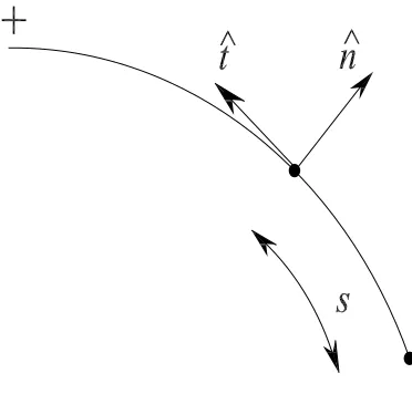
as follows. Along a curved boundary (Figure 1), the values of ∂ψ/∂x and ∂ψ/∂y
can be easily obtained from the prescribed boundary values for ψ and ∂ψ/∂n. By introducing an interpolating scheme (e.g. 1D-IRBFNs) on the boundary, one is
able to get derivatives of∂ψ/∂x and ∂ψ/∂y along the boundary such as∂2ψ/∂x∂s
and ∂2ψ/∂y∂s in which s is the arc-length of the curved boundary. A tangential
derivative of a generic functionf at a boundary point, xb, can be computed by
∂f ∂s =
∂f ∂xtx+
∂f
∂yty, (23)
wheretx =∂x/∂sandty =∂y/∂sare the twoxandycomponents of the unit vector
Replacing f with ∂ψ(xb)/∂x, we have
∂2ψ(x
b)
∂x∂s =
∂2ψ(x
b)
∂x2 tx+
∂2ψ(x
b)
∂x∂y ty, (24)
or
∂2ψ(x
b)
∂x∂y =
1
ty
∂2ψ(x
b)
∂x∂s −
∂2ψ(x
b)
∂x2 tx
, (25)
where the value of ∂2ψ(x
b)/∂x∂sis known.
Similarly, taking f as ∂ψ(xb)/∂y results in
∂2ψ(x
b)
∂x∂y =
1
tx
∂2ψ(x
b)
∂y∂s −
∂2ψ(x
b)
∂y2 ty
. (26)
From (25) and (26), one can derive the relation between∂2ψ/∂x2 and∂2ψ/∂y2 at a
boundary point
1
ty
∂2ψ(x
b)
∂x∂s −
∂2ψ(x
b)
∂x2 tx
= 1
tx
∂2ψ(x
b)
∂y∂s −
∂2ψ(x
b)
∂y2 ty
. (27)
Expression (27) can be rearranged as
∂2ψ(x
b)
∂y2 =
tx
ty
2
∂2ψ(x
b)
∂x2 +qy, (28)
whereqy is a known value defined by
qy =−
tx
t2
y
∂2ψ(x
b)
∂x∂s +
1
ty
∂2ψ(x
b)
∂y∂s . (29)
Formula (28) facilitates the computation of the value of ∂2ψ/∂y2 at a boundary
pointxb using the approximations on the x−grid line.
pointyb can be computed by
∂2ψ(y
b)
∂x2 =
ty
tx
2
∂2ψ(y
b)
∂y2 +qx, (30)
whereqx is a known value defined by
qx =−
ty
t2
x
∂2ψ(y
b)
∂y∂s +
1
tx
∂2ψ(y
b)
∂x∂s . (31)
It can be seen that, given a Cartesian grid, expressions (28) and (30) allow the
approximations of mixed derivatives in regions bounded by irregular surfaces to be
expressed in terms of the nodal values ofψ and the boundary conditions.
4.3
1D-IRBF expressions
1D-IRBF expressions on thex− andy−grid lines have similar forms. In the follow-ing, the process of deriving 1D-IRBF expressions for the stream-function variable
and its derivatives on thex−grid lines is presented in detail.
4.3.1 Pure derivatives
Along anx−grid line (Figure 2), the set of RBF centres consists of the interior points
{xi} q
i=1 and the two boundary points {xbi}2i=1. The stream-function variable is
ap-proximated using 1D-IRBFN-4s. At a boundary pointxb, there are double boundary
conditions, ψ(xb) and ∂ψ(xb)/∂x. Unlike conventional differentiated RBFNs, there
are four integration constants in the 1D-IRBFN formulation. These extra
coeffi-cients allows for the addition of some extra equations to the process of conversion of
to implement derivative boundary values b ψ b ψb c ∂ψb ∂x = b
C w,b (32)
where
b
ψ = (ψ(x1), ψ(x2),· · · , ψ(xq))T,
b
ψb = (ψ(xb1), ψ(xb2))T,
d
∂ψb
∂x =
∂ψ(xb1)
∂x ,
∂ψ(xb2)
∂x T , b C =
I1(0)(x1) · · · Im(0)(x1) x31/6 x21/2 x1 1
I1(0)(x2) · · · Im(0)(x2) x32/6 x22/2 x2 1
... . .. ... ... ... ... ...
I1(0)(xq) · · · Im(0)(xq) x3q/6 x2q/2 xq 1
I1(0)(xb1) · · · Im(0)(xb1) x3b1/6 x2b1/2 xb1 1
I1(0)(xb2) · · · Im(0)(xb2) x3b2/6 x2b2/2 xb2 1
I1(1)(xb1) · · · Im(1)(xb1) x2b1/2 xb1 1 0
I1(1)(xb2) · · · Im(1)(xb2) x2b2/2 xb2 1 0
, b
w= (w1, w2,· · · , wm, c1, c2, c3, c4)T ,
and m = q+ 2. The values of the lth-order derivative (l ={1,2,3,4}) of ψ at the interior points on the grid line are evaluated as
d
∂lψ
∂xl =Ib
(l) [4]Cb−
1 b ψ b ψb c ∂ψb ∂x
where
b
I[4](4) =
I1(4)(x1) · · · Im(4)(x1) 0 0 0 0
I1(4)(x2) · · · Im(4)(x2) 0 0 0 0
... . .. ... ... ... ... ...
I1(4)(xq) · · · I
(4)
m (xq) 0 0 0 0
, b
I[4](3) =
I1(3)(x1) · · · Im(3)(x1) 1 0 0 0
I1(3)(x2) · · · Im(3)(x2) 1 0 0 0
... . .. ... ... ... ... ...
I1(3)(xq) · · · I
(3)
m (xq) 1 0 0 0
, b
I[4](2) =
I1(2)(x1) · · · Im(2)(x1) x1 1 0 0
I1(2)(x2) · · · Im(2)(x2) x2 1 0 0
... . .. ... ... ... ... ...
I1(2)(xq) · · · Im(2)(xq) xq 1 0 0
, and b
I[4](1) =
I1(1)(x1) · · · Im(1)(x1) x21/2 x1 1 0
I1(1)(x2) · · · Im(1)(x2) x22/2 x2 1 0
... . .. ... ... ... ... ...
I1(1)(xq) · · · Im(1)(xq) x2q/2 xq 1 0
.
Expressions (33) can be rewritten in compact form
d
∂lψ
∂xl =Dblxψb+bklx, (34)
whereDblx are the differentiation matrices in the physical space, and bklx the vectors
whose components are functions of boundary conditions. It is noted that, for the
Similarly, 1D-IRBFN expressions for pure derivatives on the y−grid lines take the following forms
d
∂lψ
∂yl =Dblyψb+bkly, (35)
wherel ={1,2,3,4}.
4.3.2 Mixed derivatives
On an x−grid line, it can be seen from (20)-(22) that relevant mixed derivative to be evaluated here are∂2(∂ψ/∂y)/∂x2 and∂2(∂2ψ/∂y2)/∂x2. Approximate
expres-sions for∂ψ/∂y and ∂2ψ/∂y2 can be obtained at the interior points using (35) with
l={1,2}. At the boundary points, the values of ∂ψ/∂y are given, while the values of ∂2ψ/∂y2 can be computed using (28) in which ∂2ψ/∂x2 is evaluated using the
nodal values ofψ on the x−grid line
∂2ψ(x
b)
∂x2 =
I1(2)(xb)· · ·I
(2)
m (xb) xb 1 0 0
b
C−1
b
ψ
b
ψb
c
∂ψb
∂x
, (36)
wherexb is a boundary point and ψ,b ∂ψcb/∂x,wb and Cbare defined as before.
Let g represent ∂2ψ/∂y2 and ∂ψ/∂y. The remaining task is to form an 1D-IRBF
expression for∂2g/∂x2. This process is similar to that for the stream function which
is described in Section 4.3.1, except that there are no extra equations representing
4.3.3 Single-valued pressure equation
As shown in (18)/(19), this pressure condition involves pure and mixed derivatives
on the wall.
Using 1D-IRBFN expressions which are derived above, one can express derivatives
in (18)/(19) in terms of the nodal values of ψ. For example, the integrand of the third term in (19) can be written as
∂3ψ(x
b)
∂x3 =
I1(3)(xb)· · ·Im(3)(xb) 1 0 0 0
b
C−1
b
ψ
b
ψb
c
∂ψb
∂x
, (37)
wherexb is the boundary point on the inner wall andψ,b ∂ψcb/∂x,wbandCbare defined
as before. The vector ψbb in (37) contains the value of the stream function on the
inner cylinder, i.e. ψ(xb), that is an unknown to be found.
All associated integrals in (18)/(19) are then evaluated using the Gauss quadrature
scheme.
The pressure condition leads to a relation where the value of ψ on the inner wall is expressed as a linear combination of the values of ψ at the interior points.
4.4
Solution Procedure
The algebraic equation set resulting from the discretisation of the stream-function
formulation is nonlinear because of the presence of the convective terms. There are
two approaches widely used to handle this nonlinearity. In the first approach, all time
can be applied. In the second approach, the solution is obtained by means of time
marching. Each approach has some advantages over the other for certain problems.
In this study, fluid flow problems are considered and the second approach is applied.
1. Guess initial values of T, ψ and their spatial derivatives at time t= 0.
2. Discretise the governing equations in time using a first-order accurate
finite-difference scheme, where the diffusive and convective terms are treated
implic-itly and explicimplic-itly, respectively.
3. Discretise the governing equations in space using 1D-IRBF schemes,
Solve the energy equation (2) for T, and Solve the momentum equation (1) for ψ.
The two equations are solved separately in order to keep matrix sizes to a
minimum.
4. Check to see whether the solution has reached a steady state
CM = r
Pnip
i=1
ψ(ik)−ψ(k−1)
i
2
r Pnip
i=1
ψi(k)2
< ǫ, (38)
where k is the time level and ǫ is the prescribed tolerance.
5. If it is not satisfied, advance time step and repeat from step 2. Otherwise,
stop the computation and output the results.
driven flows in eccentric annuli with a wide range of the eccentricity. The computed
solution at the lower and nearest value ofRe/Ra is taken to be the initial solution. Internal grid points that fall very close–within a distance of h/8–to the boundary are removed.
It is well known that RBF-based schemes suffer from the so-called uncertainty or
trade-off principle. As the value of the RBF-width/shape-parameter increases, the
approximation error reduces while the condition number of the system matrix grows.
Unfortunately, there is still a lack of theory to determine the optimal value for the
RBF width. The RBF width is usually chosen by trial and error or some other
ad-hoc means. In this study, the grid size h is taken to be the MQ-RBF width. For conventional FDMs and pseudo-spectral techniques, coordinate transformations
are required to convert non-rectangular domains into rectangular ones [16,18]. The
relationships between the physical and computational coordinates are given by a set
of algebraic equations or a set of partial differential equations (PDEs), depending
on the level of complexity of the geometry. Such transformation processes are, in
general, complicated. The proposed technique can work with irregular domains in a
direct manner, i.e. without the need for using coordinate transformations. However,
the proposed technique is restricted to structured uniform or non-uniform Cartesian
grids.
5.1
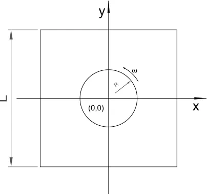
Example 1:
Steady flow between a rotating circular
cylinder and a fixed square cylinder
This test problem is employed for the investigation of accuracy of the proposed
technique in computing the value of the stream function on the inner cylinder. The
at a unit angular velocity. The stream function on the outer wall is set to zero.
Formula (18) is utilised to determine the value of the stream function on the inner
wall, denoted by ψw. This flow is governed by (3) and subject to the boundary
conditions
ψ = ∂ψ
∂x = ∂ψ
∂y = 0,
on the outer cylinder and
ψ =ψw,
∂ψ
∂x =−x, ∂ψ
∂y =−y,
on the inner cylinder. The flow is simulated with R = 0.25 and L = {0.55,1.0} using a uniform grid of 52×52. Different values of the Reynolds number, namely
1, 100, 500, 700 and 1000, are considered. Results concerning ψw obtained by the
proposed technique and the finite-difference technique [15] are presented in Table 1,
showing a satisfactory agreement. Plots for the velocity and vorticity fields for the
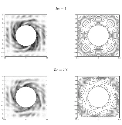
case of L= 1 andR = 0.5 at Re={1,700} are given in Figure 4.
5.2
Example 2: Natural convection in an eccentric annulus
between two circular cylinders
Natural convection is governed by the coupling of the momentum equation (velocity
field) (1) and energy equation (temperature field) (2). Solutions to natural
con-vection in concentric and eccentric annuli between two circular cylinders have been
reported using various discretisation techniques such as finite-difference methods
(FDMs) (e.g. [19,20]), finite-element methods (FEMs) (e.g. [21,22]), finite-volume
methods (FVMs) (e.g. [23,24]), boundary-element methods (BEMs) (e.g. [25,26])
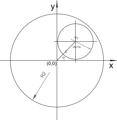
Consider buoyancy-driven flows of a Newtonian fluid between two cylinders whose
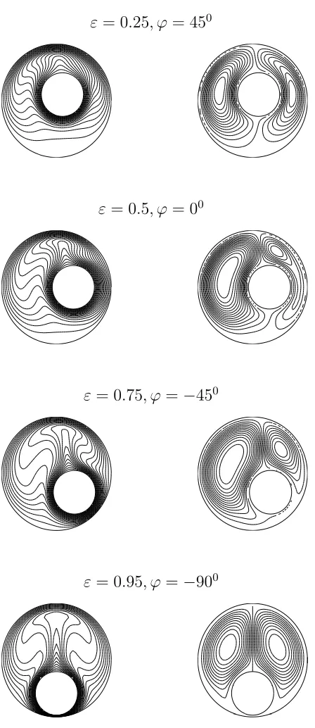
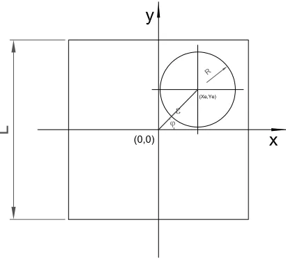
centres are separated by a distance ε (Figure 5). As shown in Figure 5, the flow geometry is defined by the following geometrical parameters: the eccentricity ε, angular position ϕ, the diameter of the outer cylinder Do and the diameter of the
inner cylinder Di. In the present work, the numerical results are reported with
P r= 0.71 and Do/Di = 2.6. A typical discretisation is shown on Figure 6a, where
no coordinate transformations are employed.
The inner and outer cylinders are heated (T = 1) and cooled (T = 0), respectively. The stream-function value at the outer cylinder is set to zero. The stream-function
value at the inner cylinder is a part of the solution and can be determined by the
single-valued pressure condition (19). The normal derivatives of the stream function
are set to zero at both walls.
One typical quantity associated with this type of flow is the average equivalent
conductivity denoted by ¯keq. This quantity is defined as (e.g. [20])
¯
keq= −
ln(Do/Di)
2π
I
∂T
∂nds (39)
The present method is first tested with the case of symmetrical flows. For such flows,
one is able to know the exact solution ofψ at the inner wall (ψw = 0), which can be
used to test numerical solvers. We employ three uniform grids of 41×41, 51×51
and 61×61 to represent the flow field. Results obtained show that the value of
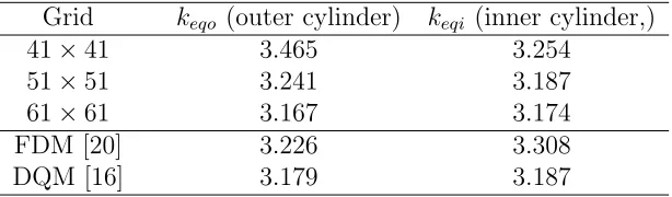
ψw is less than 10−6. For concentric cylinders, results concerning ¯keq by the present
technique together with those by FDMs [20] and DQMs [16] for Ra= 7×10⁴ are
presented in Table 2. The present solutions converge well and are in close agreement
with the other solutions. It can be seen that the IRBF results are more agreeable
to the DQ ones than the FD results. For eccentric cylinders (i.e. the centres of
the maximum value ofψ forRa= 104 between the proposed method and the DQM
[16]. Good agreement is achieved.
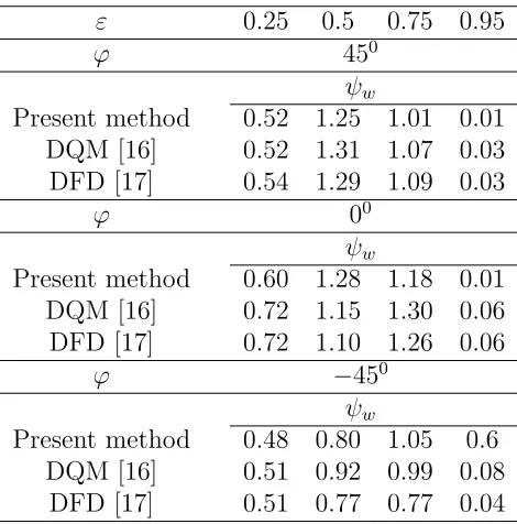
For the case of unsymmetrical flows, the value of ψ at the inner wall has non-zero value that varies with the location of the inner cylinder. Different amounts
of eccentricity (ε), namely {0.25,0.5,0.75,0.95}, and angular direction ϕ, namely
{−900,−450,00,450,900}, are employed. In Table 4, the values ofψat the inner walls
are presented and agree satisfactorily with those conducted by the DQM [16] and
the domain free discretisation method (DFD) [17]. Figure 7 shows the streamlines
and isotherms of the flow atRa= 104 using a grid of 61×61, where different values
of eccentricity and angular directions are employed. Each plot contains 21 contour
lines whose levels vary linearly from the minimum to maximum values. All plots
look reasonable when compared with those of the DQM [16].
5.3
Example 3: Natural convection in an eccentric annulus
between a square outer and a circular inner cylinder
In this example, natural convection between a heated inner circular cylinder and a
cooled square enclosure (Figure 8) is considered. An aspect ratio ofL/2R= 0.26 (L: the side length of the outer square andR: the radius of the inner circle), P r= 0.71 and Ra= 3×10⁵ are used.
The problem domain is simply replaced with a Cartesian grid (Figure 6b), where no
coordinate transformations are employed.
can be taken to be zero. Calculations are conducted on a uniform Cartesian grid of
62×62. In Table 5, the maximum values of the stream function are presented and
compared very well with those conducted by Ding [29].
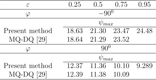
For special cases of eccentric square-circular annuli, where the centre of the inner
cylinder lies on the vertical symmetrical axis of an outer cylinder, the values of
ψmax are given in Table 6. It can be seen that the present results are in very good
agreement with those of Ding [29].
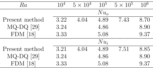
Following the work of Moukalled and Acharya [18], the local heat transfer coefficient
is defined as
θ=−k∂T
∂n, (40)
where k is the thermal conductivity. The average Nusselt number (the ratio of the temperature gradient at the wall to a reference temperature gradient) is computed
by
N u= θ
k, (41)
where θ = −H ∂T
∂nds. Since the computational domain in [18] is taken as one-half
of the physical domain, the values of N u in the present work (Table 7) are divided by 2 for comparison purposes. The present results agree well with those in [18] and
[29].
Figures 9 displays streamline and isotherm fields with different positions of the inner
cylinder for Ra = 3×10⁵. The qualitative behaviours of these fields and those in
[29] are similar. In Figure 10, the effects of time step on the convergence of the
proposed technique are investigated for the case of Ra = 1×10⁵ using a grid of
53×53. It can be seen that the present technique can work with a wide range of
the value of time step. As expected, the convergence is faster but less stable when
consumes 0.013715 (s) per iteration for a grid of 33×33, 0.0599 for 49×49 and
0.0807 for 53×53 (Intel Core 2 6300-1.86 Ghz).
For all values of the Reynolds/Rayleigh number employed in these examples, it is
observed that the solution evolves in a stable manner with relatively-large time
steps. As a result, the use of special treatments for the convection term such as the
upwind scheme is not necessary here.
6
Concluding Remarks
In this article, flows in multiply-connected domains are studied using the
stream-function formulation, one-dimensional integrated RBF approximations and
Carte-sian grids. Formulas for handling mixed derivatives in irregular regions and
bound-ary conditions for the stream-function variable are derived under the Cartesian
framework, and they are implemented effectively with 1D-IRBFNs. Attractive
fea-tures of the proposed technique include (i) simple preprocessing and (ii) the ability
to retain the PDEs in their Cartesian forms, and thus to work in a similar fashion
for different shapes of annuli. Various solutions are reported to demonstrate the
capabilities of the proposed technique.
Acknowledgements
This research is supported by the Australian Research Council. K. Le-Cao wishes
to thank the USQ, CESRC and CSIRO for a postgraduate scholarship. The authors
References
[1] Fasshauer GE. Solving partial differential equations by collocation with radial
ba-sis functions, Surface Fitting and Multiresolution Methods. Nashville:Vanderbilt
University Press; 1997.
[2] Kansa EJ. Multiquadrics- A scattered data approximation scheme with
applica-tions to computational fluid-dynamics-II. Soluapplica-tions to parabolic, hyperbolic and
elliptic partial differential equations. Computers and Mathematics with
Appli-cations 1990;19(8/9):147-161.
[3] Kosec G, Sarler B. Solution of thermo-fluid problems by collocation with
lo-cal pressure correction. International Journal of Numerilo-cal Methods for Heat &
Fluid Flow 2008;18(7/8):868-882.
[4] Le-Cao K, Mai-Duy N, Tran-Cong T. An effective integrated-rbfn
cartesian-grid discretization for the stream function-vorticity-temperature formulation
in nonrectangular domains. Numerical Heat Transfer, Part B: Fundamentals
2009;55(6):480-502.
[5] Mai-Duy N, Le-Cao K, Tran-Cong T. A Cartesian grid technique based on
one-dimensional integrated radial basis function networks for natural convection
in conccentric annuli. International Journal for Numerical Methods in Fluids
2008;57:1709-1730.
[6] Mai-Duy N, Tran-Cong T. Numerical solution of Navier-Stokes equations using
multiquadric radial basis function networks. International Journal for Numerical
Methods in Fluids 2001;37(1):65-86.
[7] Mai-Duy N, Tran-Cong T. Approximation of function and its derivatives using
radial basis function networks. Applied Mathematical Modelling
[8] Mai-Duy N, Tran-Cong T. A Cartesian-grid collocation method based on
radial-basis-function networks for solving PDEs in irregular domains. Numerical
Meth-ods for Partial Differential Equations 2007;23(5):1192-1210.
[9] Sarler B. A radial basis function collocation approach in computational fluid
dynamics. Computer Modeling in Engineering and Sciences 2005;7(2):185-194.
[10] Driscoll TA, Fornberg B. Interpolation in the limit of increasingly flat radial
basis functions. Computers and Mathematics with Applications 2002;43:413-422.
[11] Schaback R. Multivariate interpolation by polynomials and radial basis
func-tions. Constructive Approximation 2005;21:293-317.
[12] Wright GB, Fornberg B. Scattered node compact finite difference-type formulas
generated from radial basis functions. Journal of Computational Physics 2006;
212:99-123.
[13] Roger P. Spectral Methods for Incompressible Viscous Flow Series: Applied
Mathematical Sciences, Vol. 148. New York: Springer-Verlag; 2002.
[14] Ostrach S. Natural convection in enclosures. Journal of Heat Transfer
1988;110:1175-1190.
[15] Lewis E. Steady flow between a rotating circular cylinder and fixed square
cylinder. Journal of Fluid Mechanics. 1979;95:497-513.
[16] Shu C, Yao Q, Yeo KS, Zhu YD. Numerical analysis of flow and thermal fields
in arbitrary eccentric annulus by differential quadrature method. Journal of Heat
and Mass Transfer 2002;38:597-608.
[17] Shu C, Wu YL. Domain-free discretization method for doubly connected domain
[18] Moukalled F, Acharya S. Natural convection in the annulus between concentric
horizontal circular and square cylinders. Journal of Thermophysics and Heat
Transfer 1996;10(3):524-531.
[19] de Vahl Davis G. Natural convection of air in a square cavity: a
bench-mark numerical solution. International Journal for Numerical Methods in Fluids
1983;3:249-264.
[20] Kuehn TH, Goldstein RJ. An experimental and theoretical study of natural
convection in the annulus between horizontal concentric cylinders. Journal of
Fluid Mechanics. 1976;74(4):695-719.
[21] Manzari MT. An explicit finite element algorithm for convection heat transfer
problems. International Journal of Numerical Methods for Heat & Fluid Flow
1999;9(8):860-877.
[22] Sammouda H, Belghith A, Surry C. Finite element simulation of transient
natu-ral convection of low-Prandtl-number fluids in heated cavity. International
Jour-nal of Numerical Methods for Heat & Fluid Flow 1999;9(5):612-624.
[23] Glakpe EK, Watkins CB, Cannon JN. Constant heat flux solutions for
natu-ral convection between concentric and eccentric horizontal cylinders. Numerical
Heat Transfer, Part B: Fundamentals 1986;10:279-295.
[24] Kaminski DA, Prakash C. Conjugate natural convection in a square enclosure:
effect of conduction in one of the vertical walls. International Journal of Heat
and Mass Transfer 1986;29(12):1979-1988.
[25] Hribersek M, Skerget L. Fast boundary-domain integral algorithm for the
com-putation of incompressible fluid flow problems. International Journal for
[26] Kitagawa K, Wrobel LC, Brebbia CA, Tanaka M. A boundary element
for-mulation for natural convection problems. International Journal for Numerical
Methods in Fluids 1988;8:139-149.
[27] Le Quere P. Accurate solutions to the square thermally driven cavity at high
Rayleigh number. Computers and Fluids 1991;20(1):29-41.
[28] Shu C. Application of differential quadrature method to simulate natural
con-vection in a concentric annulus. International Journal for Numerical Methods in
Fluids 1999;30:977-993.
[29] Ding H, Shu C, Yeo, KS, Lu ZL. Simulation of natural convection in eccentric
annuli between a square outer cylinder and a circular inner cylinder using local
MQ-DQ method. Numerical Heat Transfer, Part A: Applications
Re 1 100 500 1000
L 0.55
ψw
Present method 0.0581 0.0582 0.0586 0.0596 FDM [15] 0.0625 0.0626 0.0621 0.0600
L 1
ψw
[image:29.595.157.438.85.219.2]Present method 0.4622 0.4617 0.4500 0.4264 FDM [15] 0.4656 0.4577 0.4465 0.4375
Table 1: Example 1 (rotating cylinder): Comparison of the stream-function values at the inner cylinder,ψw, forRefrom 1 to 1000 between the present technique (grid
of 52×52) and finite difference technique.
Grid keqo (outer cylinder) keqi (inner cylinder,)
41×41 3.465 3.254 51×51 3.241 3.187 61×61 3.167 3.174 FDM [20] 3.226 3.308 DQM [16] 3.179 3.187
[image:29.595.145.452.310.400.2]ε 0.25 0.5 0.75 0.95
ϕ −900
ψmax
Present method 22.19 20.72 18.50 15.71 DQM [16] 22.16 20.62 18.32 15.50
ϕ 900
ψmax
[image:30.595.169.427.115.250.2]Present method 11.26 9.64 8.25 7.28 DQM [16] 11.13 9.55 8.12 7.17
Table 3: Example 2 (symmetric flow, eccentric circular-circular annuli): Comparison of the maximum stream-function values,ψmax, for two special casesϕ ={−900,900}
between the present technique and DQM technique.
ε 0.25 0.5 0.75 0.95
ϕ 450
ψw
Present method 0.52 1.25 1.01 0.01 DQM [16] 0.52 1.31 1.07 0.03 DFD [17] 0.54 1.29 1.09 0.03
ϕ 00
ψw
Present method 0.60 1.28 1.18 0.01 DQM [16] 0.72 1.15 1.30 0.06 DFD [17] 0.72 1.10 1.26 0.06
ϕ −450
ψw
Present method 0.48 0.80 1.05 0.6 DQM [16] 0.51 0.92 0.99 0.08
DFD [17] 0.51 0.77 0.77 0.04
Table 4: Example 2 (unsymmetrical flow, eccentric circular-circular annuli): Comparison of the stream-function values at the inner cylinders, ψw, for ε =
{0.25,0.5,0.75,0.95} and ϕ ={−450,00,450}between the present, DQM and DFD
[image:30.595.180.415.393.631.2]ε 0.25 0.5 0.75 0.95
ϕ 450
ψmax
Present method 15.31 14.23 13.52 12.91 MQ-DQ [29] 15.32 14.35 13.61 12.98
ϕ 00
ψmax
Present method 17.00 16.99 16.87 17.18 MQ-DQ [29] 17.00 16.97 16.84
ϕ −450
ψmax
[image:31.595.169.429.130.320.2]Present method 18.50 20.09 21.02 21.61 MQ-DQ [29] 18.50 20.03 21.01 21.68
Table 5: Example 3 (eccentric square-circular annuli): Comparison of the maximum stream-function values,ψmax, for ε={0.25,0.5,0.75,0.95} and ϕ ={−450,00,450}
between the present technique and MQ-DQ technique.
ε 0.25 0.5 0.75 0.95
ϕ −900
ψmax
Present method 18.63 21.30 23.47 24.48 MQ-DQ [29] 18.64 21.29 23.52
ϕ 900
ψmax
Present method 12.37 11.36 10.10 9.289 MQ-DQ [29] 12.39 11.38 10.09
Table 6: Example 3 (eccentric square-circular annuli): Comparison of the maximum stream-function values,ψmax, for special cases ϕ={−900,900}between the present
[image:31.595.168.427.497.631.2]Ra 104 5×10⁴ 105 5×10⁵ 106
N uo
Present method 3.22 4.04 4.89 7.43 8.70 MQ-DQ [29] 3.24 4.86 8.90 FDM [18] 3.33 5.08 9.37
N ui
[image:32.595.148.448.311.446.2]Present method 3.21 4.04 4.89 7.51 8.85 MQ-DQ [29] 3.24 4.86 8.90 FDM [18] 3.33 5.08 9.37
Table 7: Example 3 (square-circular annulus): Comparison of the average Nusselt number on the outer and inner cylinders, N uo and N ui, for Ra from 104 to 106
x1 x2 xq
xb1 xb2
Figure 2: Points on a grid line consist of interior pointsxi (◦) and boundary points
Re= 1
−0.5 0 0.5
−0.5 −0.4 −0.3 −0.2 −0.1 0 0.1 0.2 0.3 0.4 0.5
−0.5 0 0.5
−0.5 −0.4 −0.3 −0.2 −0.1 0 0.1 0.2 0.3 0.4 0.5
Re= 700
−0.5 0 0.5
−0.5 −0.4 −0.3 −0.2 −0.1 0 0.1 0.2 0.3 0.4 0.5
−0.5 0 0.5
[image:36.595.123.525.170.583.2]−0.5 −0.4 −0.3 −0.2 −0.1 0 0.1 0.2 0.3 0.4 0.5
(a) (b)
ε= 0.25, ϕ= 450
ε= 0.5, ϕ= 00
ε= 0.75, ϕ =−450
[image:39.595.190.414.113.630.2]ε= 0.95, ϕ =−900
Figure 7: Example 2 (circular-circular annulus): Contour plots for the temperature (left) and stream-function (right) fields with respect different values of eccentricity
ε and angular directions ϕ for the flow at Ra = 1 ×10⁴. Each plot contains 21
ε= 0.25, ϕ =−450
ε= 0.5, ϕ= 00
ε= 0.75, ϕ= 450
[image:41.595.188.412.114.629.2]ε= 0.95, ϕ= 900
Figure 9: Example 3 (square-circular annulus): The temperature (left) and stream-function (right) fields with respect different values of eccentricity ε and angular directionϕ for the flow atRa= 3×10⁵. Each plot contains 21 contour lines whose
0 20 40 60 80 100 0
0.02 0.04 0.06 0.08 0.1 0.12
dt=0.05 dt=0.1 dt=0.5 dt=1
C
M
[image:42.595.114.475.100.349.2]Number of time steps