Multi-objective optimisation for tuning building heating and cooling loads forecasting models

Multi-Objective Optimisation for Tuning Building Heating and Cooling

Loads Forecasting Models

Saleh Seyedzadeh1,3*_{, Farzad Pour Rahimian}2_{, Parag Rastogi}3_{, Stephen Oliver}1,3_{, Ivan Glesk}1 _and

Bimal Kumar2

1_{Faculty of Engineering, University of Strathclyde, Glasgow, UK}

2_{Faculty of Engineering & Environment, Northumbria University, Newcastle, UK} 3_{arbnco, Glasgow, UK}

*email: [email protected]

Abstract

Machine learning (ML) has been recognised as a powerful method for modelling building energy consumption. The capability of ML to provide a fast and accurate prediction of energy loads makes it an ideal tool for decision-making tasks related to sustainable design and retrofit planning. However, the accuracy of these ML models is much dependant on the selection of the right hyper-parameters for specific building dataset. This paper proposes a method for optimising ML model for forecasting both heating and cooling loads. The technique employs multi-objective optimisation with evolutionary algorithms to search the space of possible parameters. The proposed approach not only tune one model to precisely predict building energy loads but also accelerates the process of model optimisation. The study utilises a simulated building energy data generated in EnergyPlus to demonstrate the efficiency of the proposed method, and compares the outcomes with the regular ML tuning procedure (i.e. grid search). The optimised model provides a reliable tool for building designers and engineers to explore a large space of the available building materials and technologies.

1.

Introduction

There have been several approaches proposed to enhance the energy efficiency of buildings in many countries during the last couple of decades. For instance in Europe, it was estimated in 2010 that 60 billion Euros could be saved annually by improving EU buildings’ energy performance by 20 per cent (X. Li, Bowers, & Schnier, 2010).

Every attempt to optimise buildings’ energy performance involves series of calculations to estimate the energy consumption and create an index such as Energy Performance Indicator (EPI) or Energy Use Intensity (EUI) from the measured data (T. Hong, Koo, Kim, Lee, & Jeong, 2015; Nikolaou, Kolokotsa, Stavrakakis, Apostolou, & Munteanu, 2015). Most prevailing optimisation methods are simulation-based where the energy-related objectives (i.e. energy consumption or gas emission) are calculated by a Building Performance Simulation (BPS) tool such as EnergyPlus, TRNSYS or ESP-r. This approach limits the computation complexity of the algorithms to BPSs’ calculation time. As such, when a large number of solutions are defined, the calculation and optimisation process may become extremely costly to handle. For this reason, most of the studies which focused on decision making for energy performance improvement of buildings either investigated basic or simple optimisation models or targeted retrofitting only one or two parts of envelopes to pare-down total calculation time and cost. It is also noted that the majority of studies targeted residential buildings, and there are only a few examples of research related to non-domestic buildings. A key component of achieving global development and meeting climate change mitigation targets is the optimisation of the building stock. This process requires significant testing and planning to deliver.

With the tremendous growth in the amount of valid and attainable datasets of structures and collection of Big Data from smart buildings, there is an increasing interest in the employment of Artificial Intelligent (AI) methods specifically Machine Learning (ML) (Seyedzadeh, Rahimian, Glesk, & Roper, 2018).

The use of ML models needs particular consideration of the accuracy and suitability of the data and relationships inferred from the data. It has been demonstrated that the process of tuning a model not only increases the predictive accuracy but also reduces model complexity, ease of use, and consistency of predictions (Seyedzadeh, Rahimian, Rastogi, & Glesk, 2019).

ML techniques have been widely used for modelling building energy loads and performance. Traditionally, the defaults values for hyper-parameters have been used in this field, however, in recent years researchers have started to tune the ML models to have more accurate predictions of energy metrics (Ahmad, Mourshed, & Rezgui, 2017; Jain, Smith, Culligan, & Taylor, 2014; C. Li, Ding, Zhao, Yi, & Zhang, 2017; Massana, Pous, Burgas, Melendez, & Colomer, 2015). Tuning ML model hyper-parameters using grid search could be very time-consuming when a complex one is chosen such as Artificial Neural Networks or models based on decision trees.

When MLs are utilised to forecasting multiple measures such as heating and cooling loads, it is required to optimise models for both the targets (Papadopoulos, Azar, Woon, & Kontokosta, 2018; Seyedzadeh et al., 2019). This procedure, in turn, increases the time required and exacerbates the usability of MLs. To address the issues mentioned above, this paper proposes a method based on an evolutionary algorithm for optimisation of ML models for accurate prediction of both heating and cooling loads. The proposed approach uses a multi-objective optimisation (MOO) to find the most appropriate hyper-parameters for Random-Forest (RF) model. The selection of RF method is due to the high precision of in prediction and the ability to simultaneously forecast multiple targets.

The next section presents a review of previous studies and issues with tuning ML models in predicting building energy consumption. That is followed by a description of the RF method, the case study, and results from our tuning approach. The final section contains recommendations and discusses future work.

2. Background and Motivation

features (X) are mapped to one or more targets variables (Y). Unsupervised learning includes techniques such as clustering, which organises data into groups based on similarities among the samples in a dataset. Unsupervised learning is applied to an unlabeled dataset, i.e., where the there are no labels to test against, while a supervised learning algorithm detects the relation between inputs and output and used this function to predict new records.

The use of machine learning models in the analysis of buildings was first used by Kalogirou et al. (1997) to estimate building heating loads considering envelope characteristic along with the desired temperature. The work (S. A. Kalogirou, 2000) was completed in 2000 by using ANNs to predict the hourly energy demand of holiday dwellings, calculated using ZID software. Kalogirou et al. (S. Kalogirou, Florides, Neocleous, & Schizas, 2001) also used ANN to estimate the daily heat loads of model house buildings with different combinations of the wall and roof types (i.e. single vs cavity walls and roofs with different insulation applied) using a typical meteorological data for Cyprus. In that study, TRNSYS software acted as an energy evaluation engine for all cases and the data validated by the comparison of one building energy consumption with the actual measurement. Since then, ANN has been widely used for estimating building heating and cooling loads (C. Deb, Eang, Yang, & Santamouris, 2016; S. M. Hong, Paterson, Mumovic, & Steadman, 2014; Paudel, Elmtiri, Kling, Corre, & Lacarrière, 2014; Yokoyama, Wakui, & Satake, 2009), Electricity demand (Mena, Rodríguez, Castilla, & Arahal, 2014; Platon, Dehkordi, & Martel, 2015), energy demand (Dombayci, 2010; Kialashaki & Reisel, 2013; Neto & Fiorelli, 2008) and overall energy performance (Khayatian, Sarto, & Dall’O’, 2016; Wong, Wan, & Lam, 2010; Yalcintas, 2006).

Support Vector Machine (SVM) for building energy forecasting was introduced by Dong et al. (2005) and adopted by several studies for prediction of cooling and heading loads (Hou & Lian, 2009; Q. Li, Meng, Cai, Yoshino, & Mochida, 2009; Xuemei, Jin-hu, Lixing, Gang, & Jibin, 2009) electricity consumption (Massana et al., 2015; Xing-ping & Rui, 2007), and energy consumption (Chen & Tan, 2017; Jain et al., 2014; H. Zhao & Magoulès, 2010).

Ensemble ML models such as RF and gradient boosted regression trees have been introduced for decades, but their use in building energy domain is recent (Deng, Fannon, & Eckelman, 2018; Papadopoulos, Azar, Woon, & Kontokosta, 2017; Tsanas & Xifara, 2012; Wang, Wang, Zeng, Srinivasan, & Ahrentzen, 2018).

Simple models with few parameters like SVM are easy to optimise, but when the number of hyper-parameters is increased the search space becomes huge. For example, to tune an RF with six hyper-parameters, a grid search will explore more than four thousands possible configurations. That is why traditionally, the researchers mostly relied on default values for those hyper-parameters. However, such models provide far more accurate results by precise tuning in comparison with SVM or Gaussian process regression (Seyedzadeh et al., 2019). Forecasting two or more building energy measures such as heating and cooling loads at one time requires even more expertise and investigation. The use of complex model and grid search for such applications is not a viable solution, due to the complexity in time as well as selection of the ideal model.

This study proposes a framework for optimising models with several hyper-parameters and ability to predict multiple targets from the same set of features concurrently.

3. Methodology

and tested using 10-fold cross-validation and five thousand randomly selected building records. In this section, first, the RF model is introduced, followed by an explanation of MOO. Then the evaluation criteria, along with the optimisation parameters, are elaborated. Finally, the description of the building dataset, which is used as the case study for the evaluation of the proposed approach will be presented.

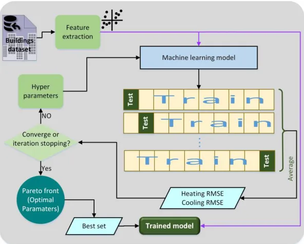
Figure 1: Schematic diagram of the proposed MOO-ML method.

3.4. Random Forest

Random forest is a collection (ensemble) of randomised decision trees (DTs). A DT is a non-parametric ML algorithm that establishes a model in the form of a tree structure. DT repeatedly divides the given records into smaller and smaller subsets until only one record remains in the subgroup. The inner and final sets are known as nodes and leaf nodes. As the precision of DT is substantially subject to the distribution of records on in the learning dataset, it is considered as an unstable method (i.e. tiny alteration in the observations will change the entire structure). To overcome this issue, a set of DTs is used and the average predicted values of all independent trees is selected as the final target. In general, RF applies bagging and boosting to combine separate models with similar information to generate a linear combination from many independent trees.

RF requires several hyperparameters to be set. The main parameter is the number of independent trees in the forest. There is a trade-off between the accuracy of model and training and predicting computational cost. Thereby, this parameter should be tuned to choose the optimal value. Other parameters include the number of features to consider when seeking for the best split, whether bootstrap (generating multiple different models from a singular training dataset) samples are used when creating trees and a minimum number of a data sample to split on nodes.

3.4. Multi-objective optimisation approach

hyper-parameters, and the most accurate model and its configuration are selected eventually. The main disadvantage of this strategy is the high time-complexity of tuning the separate models. We propose a MOO method for automated hyper

parameter selection in modelling the heating and cooling loads of a building. The proposed method reduces the time required for tuning, speeds up the model predictions and decreases human effort for implementing ML.

The general MOO problem is presented mathematically as:

Minimise:

𝐹(𝑥⃗) = [𝑓1(𝑥⃗), 𝑓2(𝑥⃗), … , 𝑓𝑚(𝑥⃗)]𝑇

Subject to

𝑔(𝑥⃗) ≤ 0 ℎ(𝑥⃗) = 0

where

𝑥_𝑖𝑚𝑖𝑛 ≤ 𝑥𝑖≤ 𝑥𝑖𝑚𝑎𝑥 (𝑖 = 1,2, … , 𝑛) 𝑥 = [𝑥1, 𝑥2, … , 𝑥𝑛]𝑇∈ 𝛩 𝑦 = [𝑦1, 𝑦2, … , 𝑦𝑚]𝑇 ∈ ψ

Here m is the number of objective functions which is three in our problem. Φ is the search space with n dimensions and identified by upper and low bounds of decision variables 𝑥𝑖(𝑖 = 1,2, . . , 𝑛).

𝑥𝑚𝑎𝑥_{= [𝑥}

1𝑚𝑎𝑥, 𝑥2𝑚𝑎𝑥, … , 𝑥𝑛𝑚𝑎𝑥]𝑇 𝑥𝑚𝑖𝑛 = [𝑥1𝑚𝑖𝑛, 𝑥2𝑚𝑖𝑛, … , 𝑥𝑛𝑚𝑖𝑛]

𝑇

Ψ is an m-dimensional vector space of objective functions and defined by Θ and the objective function f(x). 𝑔𝑗(𝑥⃗) ≤ 0(𝑗 = 1,2, . . , 𝑝) and ℎ(𝑥⃗) = 0(𝑗 = 1,2, . . , 𝑞) denotes p and q which are respectively the

number of inequality and equality constraints. If both p and q are equal to zero, then the problem is simplified as an unconstrained optimization problem.

Our tuning method involves an improved multi-objective genetic algorithm (NSGA-II) (K. Deb, 2014). Genetic algorithm is initiated by randomly generated solutions as a population and sorts them into fronts based on non-domination criteria. These solutions are evolved from one generation to another based on the objective evaluation, selection, crossover and mutation operators.

3.5. Evaluation criteria and optimisation variables

The objective functions for our optimisation problem are the accuracy of a model in the prediction of heating and cooling loads. This measure is calculated as the average root mean square (RMSE) for both heating and cooling estimations. When the MOO algorithm generates a population, each solution contains a set of RF parameters. Table 1 summarises these variables.

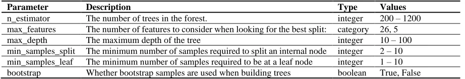
Table 1RF model hyper-parameters for tuning.

Parameter Description Type Values

n_estimator The number of trees in the forest. integer 200 – 1200 max_features The number of features to consider when looking for the best split: category 26, 5

max_depth The maximum depth of the tree integer 10 – 100

min_samples_split The minimum number of samples required to split an internal node integer 2 – 10 min_samples_leaf The minimum number of samples required to be at a leaf node integer 1 – 10 bootstrap Whether bootstrap samples are used when building trees boolean True, False

of k folds is then considered as the evaluation measure for each solution.

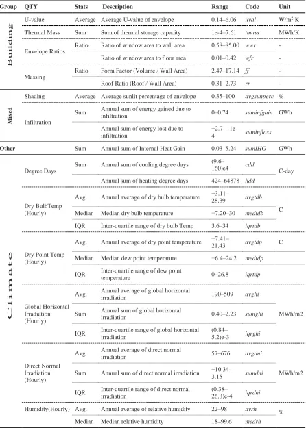
Table 2 List of input variables for model training of buildings heating and cooling loads

Group QTY Stats Description Range Code Unit

Buil

ding

U-value Average Average U-value of envelope 0.14–6.06 uval W/m2 _K

Thermal Mass Sum Sum of thermal storage capacity 1e-4–7.61 tmass MWh/K

Envelope Ratios

Ratio Ratio of window area to wall area 0.58–85.00 wwr -

Ratio of window area to floor area 0.01–0.42 wfr -

Massing

Ratio Form Factor (Volume / Wall Area) 2.47–17.14 ff -

Roof Ratio (Roof / Wall Area) 0.31–2.73 rr -

Mi

x

ed

Shading Average Average sunlit percentage of envelope 0.35–100 avgsunperc %

Infiltration

Sum Annual sum of energy gained due to

infiltration 0–0.74 suminfgain GWh

Annual sum of energy lost due to infiltration

−2.7–

-1e-4 suminfloss

Other Sum Annual sum of Internal Heat Gain 0.03–5.24 sumIHG GWh

C l i m a t e Degree Days

Sum Annual sum of cooling degree days (9.6–

160)e4 cdd _C-day

Annual sum of heating degree days 424–64878 hdd

Dry BulbTemp (Hourly)

Avg. Annual average of dry bulb temperature −3.11–

28.39 avgtdb

C

Median Median dry bulb temperature −7.20–30 medtdb

IQR Inter-quartile range of dry bulb Temp 3.6–34 iqrtdb

Dry Point Temp (Hourly)

Avg. Annual average of dry point temperature −7.41–

21.43 avgtdp C

Median Median dew point temperature −6.4–24.2 medtdp

IQR Inter-quartile range of dew point

temperature 0–26.8 iqrtdp

Global Horizontal Irradiation (Hourly)

Avg. Annual average of global horizontal

irradiation 190–509 avghi

MWh/m2 Sum Annual sum of global horizontal

irradiation 0.40–2.23 sumghi

IQR Inter-quartile range of global horizontal irradiation

(0.84–

5.2)e-3 iqrghi

Direct Normal Irradiation (Hourly)

Avg. Annual average of direct normal

irradiation 57–676 avgdni

MWh/m2 Sum Annual sum of direct normal irradiation −10.34–

3.15 sumdni

IQR Inter-quartile range of direct normal irradiation

(0.38–

26.3)e-4 iqrdni

Humidity(Hourly) Avg. Annual average of relative humidity 22–98 avrh _%

3.6. Description of the datasets

A building datasets simulated using BPS tools is utilised. This data includes 460,000 domestic and non-domestic buildings simulations characterised by 7 structural, 16 climate and 3 mixed features as presented in Table 2. The characteristics of building cases are selected from different sources including, United States Department of Energy commercial building reference database and residential houses in Geneva, Switzerland and north of Germany.

4.

Results

The results from the grid search require further investigation to select the best model. Besides, it is not possible to search every potential value for the parameters in the grid due to the size of the huge search space. Therefore, as the hyper-parameters are discretely introduced to the grid, the chance of the optimisation algorithm, which smartly selects the values is higher to reach a model with better accuracy. As expected, the best models from MOO and grid search achieves mean RMSE of 12.56 and 13.68 KW/m2 for heating and 9.28 and 9.43 for cooling predictions, respectively.

Regardless of the obtained accuracy, MOO converged on the selection of the best hyper-parameters 4.5 times faster than the time required for the grid to search the whole space. Considering the average time of 18 seconds for training and test of each fold and the size of possible combinations of the hyper-parameters as almost seven thousand, the grid is completed in 14 days whereas MOO evaluates around 1,500 solutions in 3 days.

The best hyper-parameters providing the most accurate predictions for both heating and cooling loads are as follow: n_estimators = 337, bootstrap = False, max_depth = 30, max_features = 'sqrt', min_samples_split = 3, min_samples_leaf = 1.

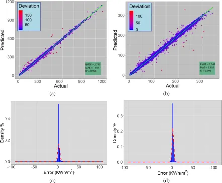
(a) (b)

(c) (d)

distributions, respectively.

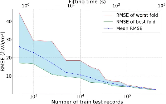
After determining RF parameters, a model is then trained and tested with 400,000 building records. The model was fit using 300,000 samples and tested over the rest. Figure 2 illustrates the results as predicted (estimated) loads against loads from the simulator (actual values), and the distribution of errors between simulated-predicted pairs. To investigate the effect of data size on the accuracy of supervised models, mean RMSE of heating and cooling is plotted against the number of train and test records which is depicted in Figure 3. Here, a 10 fold cross- validation is used in the RF model and worst, best and mean RMSE of all folds are presented. Mean training time is also displayed as the top axis for evaluating computational overhead.

Figure 3: RMSE for heating load against the total number of samples used for training

5.

Conclusion

This research addresses the gap in using ML models which require precise tuning to accurately predict building energy loads. As mentioned in the reviewed literature, most research reviewed used MLs without model optimisations, and they proposed to separately model the heating and cooling loads. This paper has proposed a method based on MOO to facilitate the process of selecting hyper-parameters, and simultaneously to optimise the model for both forecasting heating and cooling loads. The proposed approach was evaluated by implementing the random forest decision tree algorithm and testing the accuracy over a building data which was simulated using EnergyPlus. The effectiveness of our proposed approach was demonstrated through comparison with traditional grid search methods. Generating an accurate model for calculation of the energy loads with fast and robust method paves the way for more informed and productive design decisions for built environments. Furthermore, along with the optimisation algorithms, ML also offers a promising solution for efficient retrofit planning of complex buildings, where engineers are not able to carry out massive calculations readily.

Acknowledgements

The research presented in this paper was co-funded by The Data Lab (Edinburgh, UK) and arbnco Ltd (Glasgow, UK), through DataLab SFC Earmarked Grant Agreement: PO DL 00033. This work would also not be feasible without the generous PhD funding for the first author, which was co-funded by the Engineering. The Future scheme from University of University of Strathclyde and the Industry Funded Studentship Agreement with arbnco Ltd (Studentship Agreement Number: S170392-101).

References

Chen, Y., & Tan, H. (2017). Short-term prediction of electric demand in building sector via hybrid support vector regression. Applied Energy, 204, 1363–1374.

https://doi.org/https://doi.org/10.1016/j.apenergy.2017.03.070

Deb, C., Eang, L. S., Yang, J., & Santamouris, M. (2016). Forecasting diurnal cooling energy load for institutional buildings using Artificial Neural Networks. Energy and Buildings, 121, 284–297. https://doi.org/http://dx.doi.org/10.1016/j.enbuild.2015.12.050

Deb, K. (2014). Multi-objective optimization. In Search methodologies (pp. 403–449). Springer. Deng, H., Fannon, D., & Eckelman, M. J. (2018). Predictive modeling for US commercial building

energy use: A comparison of existing statistical and machine learning algorithms using CBECS microdata. Energy and Buildings, 163, 34–43. https://doi.org/10.1016/j.enbuild.2017.12.031 Dombayci, Ö. A. (2010). The prediction of heating energy consumption in a model house by using

artificial neural networks in Denizli-Turkey. Advances in Engineering Software, 41(2), 141–147. https://doi.org/https://doi.org/10.1016/j.advengsoft.2009.09.012

Dong, B., Cao, C., & Lee, S. E. (2005). Applying support vector machines to predict building energy consumption in tropical region. Energy and Buildings, 37(5), 545–553.

https://doi.org/https://doi.org/10.1016/j.enbuild.2004.09.009

Hong, S. M., Paterson, G., Mumovic, D., & Steadman, P. (2014). Improved benchmarking

comparability for energy consumption in schools. Building Research and Information, 42(1), 47–61. https://doi.org/https://doi.org/10.1080/09613218.2013.814746

Hong, T., Koo, C., Kim, J., Lee, M., & Jeong, K. (2015). A review on sustainable construction

management strategies for monitoring, diagnosing and retrofitting the building’s dynamic energy performance: Focused on the operation and maintenance phase. Applied Energy, 155, 671–707. https://doi.org/http://dx.doi.org/10.1016/j.apenergy.2015.06.043

Hou, Z., & Lian, Z. (2009). An application of support vector machines in cooling load prediction. In Intelligent Systems and Applications, 2009. ISA 2009. International Workshop on (pp. 1–4). Jain, R. K., Smith, K. M., Culligan, P. J., & Taylor, J. E. (2014). Forecasting energy consumption of

multi-family residential buildings using support vector regression: Investigating the impact of temporal and spatial monitoring granularity on performance accuracy. Applied Energy, 123, 168–178. https://doi.org/http://dx.doi.org/10.1016/j.apenergy.2014.02.057

Kalogirou, S. A. (2000). Applications of artificial neural-networks for energy systems. Applied Energy, 67(1–2), 17–35. https://doi.org/10.1016/S0306-2619(00)00005-2

Kalogirou, S., Florides, G., Neocleous, C., & Schizas, C. (2001). Estimation of Daily Heating and Cooling Loads Using Artificial Neural Networks. In Proceedings of CLIMA 2000 International Conference (pp. 15–18). Naples: Cyprus University of Technology. Retrieved from

http://ktisis.cut.ac.cy/bitstream/10488/883/3/C41-CLIMA2001.pdf

Kalogirou, S., Neocleous, C., & Schizas, C. (1997). Building Heating Load Estimation Using Artificial Neural Networks. In Proceedings of the 17th international conference on Parallel architectures and compilation techniques (Vol. 8, pp. 1–8). Retrieved from

http://www.inive.org/members_area/medias/pdf/Inive/clima2000/1997/P159.pdf

Khayatian, F., Sarto, L., & Dall’O’, G. (2016). Application of neural networks for evaluating energy performance certificates of residential buildings. Energy and Buildings, 125, 45–54.

https://doi.org/http://dx.doi.org/10.1016/j.enbuild.2016.04.067

Kialashaki, A., & Reisel, J. R. (2013). Modeling of the energy demand of the residential sector in the United States using regression models and artificial neural networks. Applied Energy, 108, 271– 280. https://doi.org/10.1016/j.apenergy.2013.03.034

Li, C., Ding, Z., Zhao, D., Yi, J., & Zhang, G. (2017). Building energy consumption prediction: An extreme deep learning approach. Energies, 10(10), 1525.

Li, Q., Meng, Q., Cai, J., Yoshino, H., & Mochida, A. (2009). Predicting hourly cooling load in the building: A comparison of support vector machine and different artificial neural networks. Energy Conversion and Management, 50(1), 90–96.

https://doi.org/http://dx.doi.org/10.1016/j.enconman.2008.08.033

Li, X., Bowers, C. P., & Schnier, T. (2010). Classification of energy consumption in buildings with outlier detection. IEEE Transactions on Industrial Electronics, 57(11), 3639–3644.

https://doi.org/10.1109/TIE.2009.2027926

a non-residential building contrasting models and attributes. Energy and Buildings, 92, 322–330. https://doi.org/10.1016/j.enbuild.2015.02.007

Mena, R., Rodríguez, F., Castilla, M., & Arahal, M. R. (2014). A prediction model based on neural networks for the energy consumption of a bioclimatic building. Energy and Buildings, 82, 142– 155. https://doi.org/http://dx.doi.org/10.1016/j.enbuild.2014.06.052

Neto, A. H., & Fiorelli, F. A. S. (2008). Comparison between detailed model simulation and artificial neural network for forecasting building energy consumption. Energy and Buildings, 40(12), 2169–2176. https://doi.org/https://doi.org/10.1016/j.enbuild.2008.06.013

Nikolaou, T., Kolokotsa, D., Stavrakakis, G., Apostolou, A., & Munteanu, C. (2015). Review and State of the Art on Methodologies of Buildings’ Energy-Efficiency Classification. In Managing Indoor Environments and Energy in Buildings with Integrated Intelligent Systems (pp. 13–31). Springer International Publishing. https://doi.org/https://doi.org/10.1007/978-3-319-21798-7 Papadopoulos, S., Azar, E., Woon, W.-L., & Kontokosta, C. E. (2017). Evaluation of tree-based

ensemble learning algorithms for building energy performance estimation. Journal of Building Performance Simulation, 1493, 1–11.

https://doi.org/https://doi.org/10.1080/19401493.2017.1354919

Papadopoulos, S., Azar, E., Woon, W.-L., & Kontokosta, C. E. (2018). Evaluation of tree-based ensemble learning algorithms for building energy performance estimation. Journal of Building Performance Simulation, 11(3), 322–332.

Paudel, S., Elmtiri, M., Kling, W. L., Corre, O. Le, & Lacarrière, B. (2014). Pseudo dynamic

transitional modeling of building heating energy demand using artificial neural network. Energy and Buildings, 70, 81–93. https://doi.org/10.1016/j.enbuild.2013.11.051

Platon, R., Dehkordi, V. R., & Martel, J. (2015). Hourly prediction of a building’s electricity consumption using case-based reasoning, artificial neural networks and principal component analysis. Energy and Buildings, 92, 10–18.

https://doi.org/http://dx.doi.org/10.1016/j.enbuild.2015.01.047

Seyedzadeh, S., Rahimian, F. P., Glesk, I., & Roper, M. (2018). Machine learning for estimation of building energy consumption and performance: a review. Visualization in Engineering, 6(1), 5. https://doi.org/https://doi.org/10.1186/s40327-018-0064-7

Seyedzadeh, S., Rahimian, F. P., Rastogi, P., & Glesk, I. (2019). Tuning Machine Learning Models for Prediction of Building Energy Loads. Sustainable Cities and Society.

Tsanas, A., & Xifara, A. (2012). Accurate quantitative estimation of energy performance of residential buildings using statistical machine learning tools. Energy and Buildings, 49, 560– 567. https://doi.org/https://doi.org/10.1016/j.enbuild.2012.03.003

Wang, Z., Wang, Y., Zeng, R., Srinivasan, R. S., & Ahrentzen, S. (2018). Random Forest based hourly building energy prediction. Energy and Buildings, 171, 11–25.

https://doi.org/https://doi.org/10.1016/j.enbuild.2018.04.008

Wong, S. L., Wan, K. K. W., & Lam, T. N. T. (2010). Artificial neural networks for energy analysis of office buildings with daylighting. Applied Energy, 87(2), 551–557.

https://doi.org/https://doi.org/10.1016/j.apenergy.2009.06.028

Xuemei, L. X. L., Jin-hu, L. J. L., Lixing, D. L. D., Gang, X. G. X., & Jibin, L. J. L. (2009). Building Cooling Load Forecasting Model Based on LS-SVM. Asia-Pacific Conference on Information Processing, 1, 55–58. https://doi.org/https://doi.org/10.1109/APCIP.2009.22

Yalcintas, M. (2006). An energy benchmarking model based on artificial neural network method with a case example for tropical climates. International Journal of Energy Research, 30(14), 1158– 1174. https://doi.org/10.1002/er.1212

Yokoyama, R., Wakui, T., & Satake, R. (2009). Prediction of energy demands using neural network with model identification by global optimization. Energy Conversion and Management, 50(2), 319–327. https://doi.org/10.1016/j.enconman.2008.09.017

Zhao, H.-X., & Magoulès, F. (2012). Feature Selection for Predicting Building Energy Consumption Based on Statistical Learning Method. Journal of Algorithms & Computational Technology, 6(1), 59–77. https://doi.org/10.1260/1748-3018.6.1.59