Interferometric study of density fluctuations in a tokamak plasma

(1)

INTERFEROMETRIC STUDY OF

DENSITY FLUCTUATIONS IN A

TOKAMAK PLASMA

by

Raffi Nazikian

A thesis submitted for

the degree of Doctor of Philosophy at

the Australian National University

(2)

e ^ y C

/ ^

^/t^ / ^ y ^ ur^-'

y # V z

(3)

-D e c la ra tio n

I declare that, except where explicitly stated, this thesis is my own original work

and th at no part of it has been previously accepted or presented for the award of

any other degree or diploma, and that no material previously published or written

by another person is included. Chapter 2 of the thesis presents a description of

the LT-4 tokamak which is largely a synopsis of research reports and publications

produced by the laboratory and constitutes the work of a large number of peo

ple. Chapter 3, on the theory of scattering from plasma inhomogeneities, is a

distillation of im portant results produced in collaboration with Dr. John Howard

and Dr. L. E. Sharp towards the production of a book titled “Forward Angle

Collective Scattering on Fusion Plasmas” which will be published as part of the

Adam Hilger series on plasma physics.

Rafft Nazikian

(4)

A c k n o w l e d g e m e n t s

In a large laboratory like this one, there are lots of people who in some way

contributed to the successful completion of this thesis and who created an inter

esting and enjoyable environment in which to work.

First and foremost, I would like to thank my supervisor, Dr. Les Sharp, for

giving me the opportunity to work in one of the the most exciting and interesting

areas of experimental plasma research; the interferometric imaging and charac

terization of density fluctuations in Tokamak plasmas. W ithout his insight and

vision to build such an interferometer, this work would never have been carried

out in Australia.

I would like to thank my head of department, Dr. Sydney Hamberger, for his

wisdom, guidance, friendship and very real concern for my well being, and the well

being of all my PHD colleagues over the years. Of those, I would like to extend a

special thanks to Shi Xue-hua and her family for making me feel a part of their

family and for extending to me their infinite generosity, warmth and friendship.

I would like to make a very special acknowledgement to my wife, Fumiko, for

instilling in me a sense of optimism and purpose which has supported me and

which will sustain me for all the years to come.

I would like to extend my strongest gratitude to Dr. John Howard for his

guidance, support, and close collaboration throughout the last year. I owe much

of my scientific development to him, and I hope th at our collaboration will be as

fruitful in the future as it has been up till now.

The close technical support I received from the laboratory technicians was

essential for the success of the project, and I especially thank Eddy Wedhom for

his assistance throughout all stages of the construction and commissioning of the

interferometer. On the electronics side I would like to thank Clint Davies for

battling with the noise problems of the detectors and for finally winning; Ray

Kimlin for constructing many of the filters and amplifiers used in the experiment;

and Gerry McCluskey and the technicians for operating the homopolar generator.

(5)

who operated and maintained the old and dying homopolar generator, keeping

it free of major breakdowns, and allowing me a clear and uninterrupted run on

the tokamak before its decommissioning. The technical assistance provided by

David Vender in operating the tokamak single handedly was invaluable to the

success of the research program. His expertise and clear understanding of the

machine with all its idiosyncrasies freed me to concentrate on the operation of the

interferometer.

Finally, it is with some sadness and trepidation that I leave this campus and

its tranquil environment. This university has provided me with an idyllic envi

(6)

A b s tr a c t

Density fluctuations in the LT-4 tokamak plasma are investigated using a Phase

Scintillation Interferometer operating at 10.6/Ltm which is sensitive to density fluc

tuations of <5he/ n e > 10~4. The plasma is imaged across a linear detector array

which can be rotated to record projections in any direction, from toroidal to

poloidal.

The theory of forward scattering from plasmas is developed from the Rytov

approximation and aspects of the Fourier diffraction projection theorem relevant

to plasma scattering. The result is a clear conceptual picture of diffraction from

arbitrary extended refractive media, from which im portant analytical tools are

developed.

The Phase Scintillation Interferometer is used to image density perturbations

produced by large scale magnetohydro dynamic (MHD) modes in the plasma asso

ciated with Mimov oscillations. Structural characteristics are determined, and a

comparison between experimental and computed projections of the Dubois model

is made which shows th at the density fluctuations are consistent with a model of

rotating magnetic islands. Island widths and local magnetic field fluctuations are

determined and are found to compare well with measured poloidal magnetic field

fluctuations.

The interferometer is used in conjunction with other diagnostics to investi

gate minor and major disruptions in LT-4. The time frequency distribution is

introduced as an im portant analytical tool in the characterization of the various

regimes of MHD activity. Frequency and amplitude variations of an m = 3 mode

during current rise appear correlated with variations in toroidal loop voltage. The

mode is also found to persist throughout the whole discharge and to play a part

in mode locking which precedes major disruptions. Mode frequencies are found

(7)

minor and major disruptions are identified. A strong m — 1 type of internal

relaxation is found to follow rapid growth and locking of an m = 2 mode during

minor disruptions.

The interferometer is also applied to the measurement of fine scale density

fluctuations in the LT-4 tokamak during periods of low level MHD activity. Line

integral measurements indicate an edge fluctuation level of about 10% and broad

band spectra typical of strong turbulence. Anisotropy in the spectrum of fluc

tuations perpendicular to the magnetic field is observed. This observation runs

counter to reported measurements of isotropic fluctuations made on other toka-

maks using small angle scattering techniques. Very long correlation lengths along

the field lines are observed, which are consistent with nearly all models of tur

bulence in tokamak plasmas. The images are numerically filtered so as to isolate

(8)

C hapter 1

IN T R O D U C T IO N

and after the initial optimism for the machine, fundamental problems still persist

with MHD instabilities and anomalous transport1 of particles and energy from

the plasma.

Although the role instabilities play in the density and current limits of toka-

mak plasmas are fairly well understood[2, 3], the role of instabilities in anoma

lous transport remains poorly understood. The problem is not least compounded

by the experimental difficulties in determining the nature of fluctuations in the

plasma responsible for the enhanced transport. The hope of finding conclusive

evidence for turbulence driven transport has motivated the development of scat

tering diagnostics for tokamaks for at least a decade[4, 5]. Such techniques, to this

day, utilize the angular scattering of radiation from refractive index variations to

directly measure the spectrum of plasma fluctuations within a scattering volume.

Unfortunately, to achieve reasonable spatial resolution whilst trying to observe

larger scale length structures expected in large tokamaks, the beam wavelength

must also be made longer. However, high density fusion type plasmas presents a

limit to the m a x im u m wavelength one can use due to operation near the critical

density limit. A compromise seems to be in the far infrared (FIR) region of the

spectrum applied most successfully on the Text tokamak[6] , however, even by

using FIR sources, the small scattering angles involved for large scale structures

would provide insufficient spatial resolution for large machines like T F T R and

JET.

(12)

Imaging diagnostics can in theory produce high resolution images of plasmas

using tomographic techniques, however, in practice, tomography of structures

sm all compared with the plasma minor radius would be exceedingly costly to

implement and technically very challenging to say the least. The application of

imaging techniques towards the analysis of microfluctuations in tokamak p la sm a s

using a single probe beam has been demonstrated as a useful diagnostic on the

TCA and LT-4 tokamaks [7, 8]. Although tomographic recovery of local fluctua

tion levels are not possible with such s y s te m s without a large amount of a priori

information, still the methods axe very useful in determining the structure of laxge

scale MHD modes as well as to some extent the spatial distribution of sm all scale

structures.

Curiously, the measurement of large scale MHD modes relevant to the macro

scopic stability of plasm as has been left to arrays of X-ray detectors and Mimov

coils[9, 10], whilst interferometers have been used principally for measuring mpan

line integral densities. Early attem pts at using interferometers to obtain spatially

resolved plasma perturbations used an array of independent beams which could

only be used for resolving structures of the scale size of the p la sm a and effectively

filtered out small scale density fluctuations [11]. On the other hand, scattering

diagnostics, of use in determining power spectra of plasma fluctuations were of

little use in the analysis of large scale MHD activity.

The development and application of an interferometer capable of imaging both

small scale density fluctuations characteristic of plasma turbulence, as well as

narrow band, large scale MHD activity constitutes the scope of this thesis. The

diagnostic developed for the purpose is a “Phase Scintillation Interferometer”

operating at 10.6/xm with a phase sensitivity of 10“8 radians. The interferometer

was first proposed by Sharp [12] as an extension to work already performed on

Cleo using microwaves to scatter from plasma fluctuations. The choice of the

probing wavelength and the method of detection, (imaging instead of far field

scattering) follows naturally from the theory of interplanetary scintillation[13],

originally developed to study refractive index variations in the earths ionosphere,

(13)

stellar radio sources. The radio wavelengths were short enough that the ground

stations were effectively in the optical near field of the ionosphere, where density

variations in the ionosphere modulated the intensity of the transm itted radiation.

The modulations were observed to drift across the ground and the drift velocity

of ionospheric irregularities were determined using multiple observer points and

correlation techniques [14].

The main problem with imaging devices is their inability to provide localized

measurements along the line of sight. The problem is common to many fields of

physics grouped under the very general field of inverse scattering and tomography.

Some related fields include,

• Interstellar and interplanetary scintillations,

• Ultrasonic tomography,

• Seismology,

• and X-ray crystallography

just to name a few. In some cases a known source is used to probe the medium in

a non-perturbing way such as in seismology or plasma scattering, whilst in others,

emissions from extended objects axe used such as in X-ray tomography of plasmas.

Plasma scattering in the laboratory is only one aspect of a subclass of inverse

scattering problems where the scattered field conforms to solutions of the inho

mogeneous Helmholtz equation[15]. Although the central problem of scattering

theory is finding solutions to the inverse scattering problem, this in general is too

difficult to solve except by the use of many a priori conditions, and by perform

ing multiple simultaneous projections of the plasma. Such problems are called

illconditioned as inversions have to be produced with typically insufficient data

for a complete determination of the source. Instead, we adopt the typical, and

much simpler approach of restricting ourselves to the fully deterministic problem

of obtaining the form of the scattered radiation from a known distribution, and

then using this knowledge to infer properties of the scatterer which are conveyed

(14)

In this thesis, we present a general formalism in which the diffracted field from

an arbitrary, extended medium can be determined in a simple way by use of the

Fourier diffraction projection theorem (FDPT) given that the scatterer satisfies

certain weak constraints. This formalism provides insight into how tomography

m ay be performed on tokamak plasmas without the requirement th at line integral

projections of the medium be formed.

The foundations of optical scattering from waves in transparent media may

be traced back to the early 1930’s when Brillouin first proposed th at light waves

would scatter from transparent waves in the same way th at X-rays were observed

to scatter from crystals. However the foundational work on the diffraction of light

from waves in transparent media is due to Raman and N ath where they correctly

noted th at waves in transparent media acted as phase gratings to the incident

radiation, and produced a theory which for the most part explained the complex

scattered fields which were observed experimentally even from strong phase per

turbing screens. An excellent review of the history of this era and many references

may be found in Bergmann[16]. The representation of the scattering medium as a

transparent thin phase grating also forms the basis of modem investigations into

far forward scattering from plasmas by very high frequency laser beams[17, 18,19],

where the plasma is represented as a thin refractive screen.

The construction of a phase scintillation interferometer on the LT-4 Toka

mak was motivated by a need to spatially resolve the high order modes thought

responsible for anomalous transport. A high priority was to observe turbulent

fluctuations present in the plasma with the hope of identifying non-sinusoidal

‘coherent’ structures[20, 21] not readily determined by power spectral techniques

such as microwave scattering.

Chapter 2 provides an overview of the LT-4 Tokamak. The principal diagnos

tics on LT-4 are presented and the limitations of the diagnostics in determining

the nature of plasma instabilities and fluctuations are discussed. There is also

an overview of the characteristic regimes of MHD activity in LT-4. The LT-4

tokamak, like many other smaller tokamaks, tends to disrupt when the q at the

(15)

which, is used to characterize the various plasma regimes.

The theory of forward angle scattering from plasmas and its relation to the

Fourier diffraction projection theorem is discussed in chapter 3. The concept

of the Rytov phase is introduced, and the conditions under which the Rytov

approximation can be considered a good approximation to the scattered field is

discussed. It is shown that the solution in the Rytov approximation is more general

than the solution for the scattered field in the Bom approximation, and describes

both large phase shift interferometry as well as large angle scattering within the

one formalism. The expression for the Rytov phase is then used to characterize

the performance of a wide range of optical diagnostics used on plasmas. These

methods and their application to fusion plasmas are reviewed.

Chapter 4 presents a detailed discussion of the phase scintillation interferom

eter and its operation on the LT-4 tokamak. Certain anomalies appeared in the

diffracted field from sound waves which lead to the identification of adverse effects

due to non-Gaussian beam profiles, and a theoretical framework is provided for

the analysis of truncated gaussian beams.

Chapter 5 centers on the interferometric study of low order MHD activity

in LT-4. An analysis of MHD mode activity is presented and an m = 2 island

is identified from its projections. The projections axe shown to conform with a

modified form of the Dubois model, extended to model m > 2 tearing modes. The

assumption made in this work is that the density isobars correspond closely to

magnetic flux surfaces. For the proper tomographic analysis of the MHD modes

in LT-4, a knowledge of their instantaneous frequencies axe required. Although

MHD activity in tokamak plasmas axe spectrally non-stationary, little in the way

of applying joint time frequency domain (TFD) analysis of MHD signals has taken

place. It is found that the TFD analysis of the MHD data allows a convenient

categorization of the various regimes of plasma activity.

Finally in chapter 6, fine scale density fluctuations are examined. The main

aim is to produce images of small scale density perturbations. The motivation

for imaging is th at it may be possible to resolve the nature of the instabilities

(16)

discussion of scattering from random media is presented, and a new method is

introduced whereby the location of thin random phase screens may be obtained

(17)

B ib lio g r a p h y

[1] L. A. Artsimovich and et. al., “(proc. int. conf., 3rd, novosibirisk, ussr, vol.

1),” in Plasma Physics and Controlled Nuclear Fusion Research, p. 157, IAEA

Vienna, 1969. English translation.: Nucl. Fusion Special Suppl. 17 (1969).

[2] C. Z. Cheng, H. P. Furth, and A. H. Boozer, “Mhd Stability Regime of the

Tokamak,” Plasma Physics and Controlled Fusion, vol. 29, pp. 351-366, 1985.

[3] M. Persson, Resistive MHD Stability {or Rotating Plasmas. PhD thesis,

Chalmers University of Technology, Goteborg, Sweden, November 1987.

[4] E. Mazzucato, “Spectrum of Small-Scale Density Fluctuations in Tokamaks,”

Phys. Rev. Lett., vol. 48, p. 1828, 1976.

[5] V. G. Zhukovskii and V. A. Rtishchev, “Diagnostics of Tokamak Plasmas

based on th e R adiation Scattered b y D en sity F lu ctu a tio n s,” S o vie t Journal

of Plasma Physics, vol. 14, p. 276, 1988.

[6] D. L. Brower, W. A. Peebles, and N. C. J. Luhmann, “Observation of Large

Amplitude, Narrow band Density Fluctuations in the Interior of Ohmic Toka

mak Plasmas,” Phys. Rev. Lett., vol. 55, p. 2579, 1985.

[7] H. Weisen, “Turbulent Density Fluctuations in the TCA Tokamak,” Plasma

Physics and Controlled Fusion, vol. 30, p. 293, 1988.

[8] R. Nazikian and L. E. Sharp, “C0 2 Laser Scintillation Interferometer for the

Measurement of Density Fluctuations in Plasma Confinement Devices,” Rev.

Sei. Instrum., vol. 58, p. 2086, 1987.

[9] R. S. Granetz and P. Smeulders, “X-ray Tomography on JET,” Nuclear Fu

(18)

[10] H. Ku.wah.ara, A. D. Ch.eeth.am, and A. H. Morton, “Observation of

m = 7 /n = 3 , m = 5 /n = 2 , and m = 3 /n = l mhd modes During Current Ramp

ing in the LT-4 Tokamak,” Nuclear Fusion, vol. 26, p. 1092, 1986.

[11] A. R. Jacobson, “Interferometric Studies of Plasma Density Fluctuations

Propagating along the Major Radius in ZT-40M using Time Delayed Correla

tion Techniques,” Plasmas Physics and Controlled Fusion, vol. 24, pp. 1111—

1131, 1982.

[12] L. E. Sharp, “The Measurement of Large-Scale Density Fluctuations in

Toroidal Plasmas from the ’’phase scintillations” of a Probing Electromag

netic Wave,” Plasmas Physics and Controlled Fusion, vol. 25, p. 781, 1983.

[13] E. E. Salpeter, “Electron Density Fluctuations in a Plasma,” Physical Review,

vol. 120, p. 1528, 1960.

[14] R. V. E. Lovelace, Interplanetary Scintillations. PhD thesis, Cornell Univer

sity, Ithaca, N.Y., USA, 1970.

[15] H. P. Baltes, ed., Inverse Scattering Problems in Optics. Springer-Verlag,

1980.

[16] L. Bergmann and S. Hatfield, Ultrasonics. John Wiley and Sons, Inc., 1948.

[17] D. E. Evans, H. M., and H. E., “Fourier Optics Approach to Fax Forward

Scattering and Related Refractive Index Phenomena in Laboratory Plasmas,”

Plasma Physics and Controlled Fusion, vol. 24, pp. 819-834, 1982.

[18] B. W. James and C. X. Yu, “Diffraction of Laser Radiation by a Plasma

W ave- the Near Field and Far Field Limiting Cases,” Plasma Physics and

Controlled Fusion, vol. 27, p. 557, 1985.

[19] Y. Sonoda, Y. Suetsugu, K. Muraoka, and M. Akazaki, “Application of the

Fraunhofer Diffraction Method for Plasma Wave Measurements,” Plasmas

Physics and Controlled Fusion, vol. 25, pp. 1113-1132, 1983.

[20] J. Jimenez, ed., The Role of Coherent Structures in Modelling Turbulence

(19)

[21] S. L. Zweben, “Search for Coherent Structure within Tokamak Plasma Tur

(20)

C hapter 2

TH E LT-4 T O K A M A K

The LT-4 tokamak is one of many tokamaks currently operating around the world

designed to study the properties of toroidally confined plasmas. The operational

parameters of LT-4 allows for the investigation of equilibrium, stability and trans

port processes in fully ionized hot plasmas. These studies axe of m ajor relevance

to the thermonuclear fusion p r o g r a m .

A brief description of the LT-4 Tokamak is presented followed by an outline

of some im portant diagnostics on the machine. An overview of the operational

regimes of LT-4 together with some characteristic MHD activity is presented and

the chapter finishes with a discussion of phase scintillation interferometry on LT-4.

2 .1 D e s c r ip t io n o f A p p a r a tu s

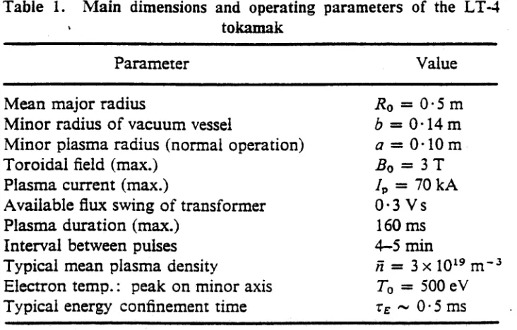
The main dimensions and operating conditions of the LT-4 tokamak are listed in

table 1.

As a thin high resistivity vacuum vessel was used on LT-4, the location of the

plasma column was stabilized during normal operation to within 1mm vertical

or horizontal displacement by use of external windings which automatically feed

back on plasma position shifts[1].

The vacuum vessel’s cutoff frequency is about 30kHz whilst most Mimov os

cillations are below this, so th at the signals remain unattenuated.

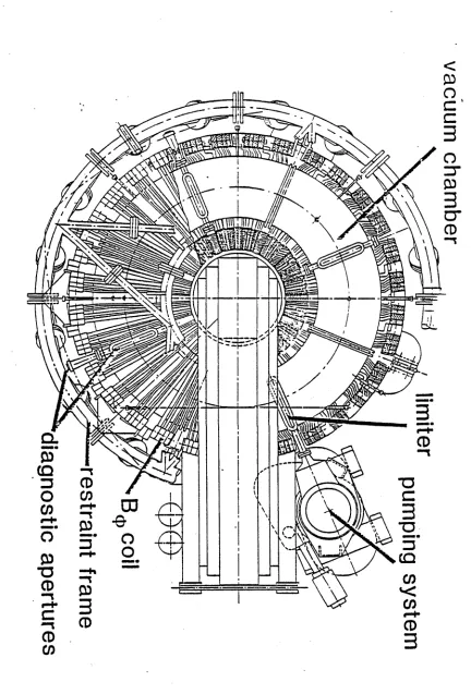
Fig. 2.1 shows a cut away view of the tokamak, exposing some of the 128

TF coils, the location of diagnostic ports, and the iron core. A large num ber of

coils were used to minimize field ripple which can be a problem for a system of

(21)

Table 1. Main dimensions and operating parameters of the LT-4

» tokamak

Parameter Value

Mean major radius R 0 = 0 • 5 m

Minor radius of vacuum vessel b = 0-14 m

Minor plasma radius (normal operation) a — 0-10 m

Toroidal field (max.) Bo = 3T

Plasma current (max.) /p = 70 kA

Available flux swing of transformer 0*3 Vs

Plasma duration (max.) 160 ms

Interval between pulses 4-5 min

Typical mean plasma density n = 3 x 1019 m -3

Electron temp.: peak on minor axis T0 = 500 eV

Typical energy confinement time rE ~ 0- 5 ms

Table 2.1: Main dimensions and operating conditions of the LT-4 tokamak

approaches the lifetime of the plasma. Diagnostic access to the plasma is via four

sets of 200x20mm rectangular vertical viewing ports with 18 9.5mm diameter ports

providing tangential views of the plasma. The plasma minor radius is confined to

10cm by a stainless steel limiter with an adjustable vertical limiter which can be

used to modify the minor radius of the plasma.

A maximum operating toroidal field of 3T was supplied by the Canberra

ho-mopolar generator operating with a cycle time of about 5 minutes. The plasma

current is the secondary of a transformer whose primary current is supplied by

capacitor banks and a mercury arc mains rectifier power supply [2]. The plasma

current attains its maximum value within 15 ms and the pulse length ( about 100

ms) is set by the saturation of the iron core.

2.2 P rin cip al D iagn ostics

The diagnostics on LT-4 can be divided into two groups. The first and simplest,

both in terms of construction and analysis, are various magnetic pick up loops

[image:21.562.100.466.113.347.2]

(22)

volt-d

ia

g

n

o

st

ic

a

p

e

rt

u

re

s

₃

Figure 2.1: Plan view of LT-4 showing the iron core, toroidal field coils, restraint frame and vacuum chamber.

v

ac

u

m

c

h

am

b

[image:22.562.73.505.45.682.2]

(23)

Mode Coils, 0 = 90* m = 1,2, 3, 7v

M16 Coils, 0=45*

Limiter, 0=22,5*

Mode Coils

core

0 = 180

A -16 ch SX array, 0 = 202,5 B- 7 ch SX array, 0 =292,5

x = N8 Coils

[image:23.562.47.508.59.462.2]

M8 Coils, 0 = 191

Figure 2.2: Arrangement of diagnostics on LT-4.

age, plasma current and plasma position. Loop voltage is obtained by measuring

the poloidal flux changes using four toroidal coils located at R=39, 61 cm and

z = ± llc m . Plasma current is obtained by numerical integration of the voltage

signal from a Rogovskii coil located outside the vacuum vessel. The plasma’s

position is determined by suitably located sine and co-sine coils on the vacuum

vessel. A description of the various pickup coils used on tokamaks can be found

in Hutchinson’s thesis[3].

Various arrays of small Mimov coils (100 turns, 3.2mm radius) are arranged

azimuthally and poloidally outside the vacuum vessel to detect local variations in

the poloidal magnetic field (Be) at a minor radius of 14.5 cm, well outside the

plasma. Two sets of coils are arranged poloidally, called M16 ( 16 individually

monitored equispaced coils) and M8 at ^ — 45° and 191° respectively (see Fig.

2.2). Another array (N8) consists of 8 equispaced toroidal coils. A single magnetic

probe is also mounted inside the vacuum vessel to pick up any high frequency

(24)

18 Channel D etector Array

SSB D etector Slit and 12,5

Be window »

Lead shield Positions

Insulating flange

250mm 252 mm

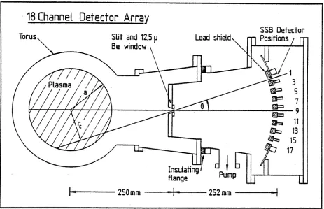
Figure 2.3: Schematic diagram of the soft X-ray array on LT-4.

The only diagnostic available which measures rapid internal variations in the

core of the plasma is the 18 channel soft X-ray (SXB.) detector array. Fig. 2.3

provides a schematic view of the soft X-ray diagnostic.

Unfortunately, as the X-ray emissivity depends on Te, ne, Z^g, and also on

the recombination of ions and impurity radiation, it is difficult to deduce absolute

parameters within the plasma[4].

The only density measuring device routinely used on LT-4 is a rotating grating

HCN Mach-Zehnder interferometer, operating at A = 337/mi, [5] providing single

point, line integral density measurements w it hin a band width of 1 kHz and able

to resolve line integral density fluctuations greater than 1013 cm-2. Typical line

integral densities for LT-4 are 5 x l0 14 cm-2.

[image:24.562.62.525.115.414.2]

(25)

light from the plasma using a Q-switched ruby laser operating at A = 694.3 nm ,

where the scattered light is detected at 90° to the beam direction. The laser beam

is focussed at the plasma mid plane and can be located at any one of three major

radial positions. The scattered spectrum is measured using a series of prisms and

photomultiplier tubes. The thermal velocities of electrons in LT-4 are low enough

that they can be considered non-relativistic to the extent th at the relativistic blue

shift in the s p e c t r u m is entirely negligible.

Hard X-rays (>100keV) are detected using a Nal scintillation photomultiplier.

A fuller description of the LT-4 diagnostics including ECE spectroscopic mea

surements can be found in the literature[2]. Fig. 2.2 gives the location of most

diagnostics on LT-4.

2.3 M H D A c tiv ity a n d F lu c tu a tio n M e a s u re m e n ts

In LT-4 the plasma current is controlled from an external power supply whilst

density is controlled by adjusting a programmable rate of gas puffing during the

pulse. It can be seen from the Hugill diagram (Fig. 2.4), th at for LT-4 (or any

other tokamak) to achieve high currents and densities, it is necessary for the Hugill

trajectory of the discharge to pass through a very narrow window. This window

is unfortunately a very strong function of the impurity level in the plasma and

impurities are a major problem for tokamaks. A discussion of impurities and

plasma confinement can be found in a review by Hugill[6]. In Fig. 2.4, q(a)

represents the safety factor at the plasma’s edge and refers to the average helicity

of field lines in the toroidal geometry where q(r) = r B r / R B o and where Bt

and Be refer to the toroidal and poloidal field components at a minor radius

r. The motivation for achieving low q operation in ohmic plasmas is to obtain

higher tem peratures and hence higher ß. In scanning the various safety factors

and density ranges in LT-4, the toroidal current was held fixed to maintain a

roughly constant power input to the plasma whilst the toroidal magnetic field was

varied by adjusting the rotor speed of the homopolar generator. From scans in

the toroidal field and plasma density, four m ajor operating regimes in LT-4 have

(26)

Figure 2.4: Hugill diagram of LT-4 showing the trajectory of a plasma discharge and boundary curves within which stable operation can be maintained.

The four basic regimes and their location in the Hugill diagram axe clearly

marked in Fig. 2.4. The regimes are identified by their distinct MHD activity

as can be seen from shot data in Fig. 2.5 taken for the discharge in the Hugill

diagram of Fig. 2.4.

• Regime I: 3.6 > q(a) > 2.9

This regime is characterized by little detectable activity on the magnetic coils

except for weak irregular signals. We will return to a discussion of these ‘irregular’

signals in chapter 5 where non-stationary spectral analysis techniques are used to

identify coherent structures in the Mimov coil data.

The soft X-ray signals show strong sawtooth activity at ~ 5kHz accompanied

by weak precursor oscillations at ~ 20kHz. Sawtooth oscillations in the plasma

centre cure indicative of a q on axis of about one and a peaked current profile[7].

The q = 1 surface is located at about r = 3cm, and is inferred from the inversion

[image:26.562.77.488.33.349.2]

(27)

(kA) 3 0

-V,

2 0

-(v)

10(mm) 1

-q(a)

3 .

Time (ms)

(28)

q(a=9,5cm)

F ig u r e 2.6: Maximum percentage poloidal field variation in the four regimes mapped against

?(o)

• Regime II: 2.9 > q(a) > 2.8

This regime is characterized by small amplitude m =3 oscillations on the Mimov

coils with a Bq/ Bq ~ 0.05% and frequencies in the range of 40 kHz. The X-ray

data shows stronger and more regular oscillations around 20kHz superimposed

on the sawtooth signals which are diminished in amplitude compared to regime I

sawteeth.

• Regime III: 2.8 > q(a) > 2.5

This regime is by fax the most active, exhibiting pronounced MHD activity

with Be/Be ~ 0.3% with a significant m =2 component. This regime is charac

terized by a sudden growth and saturation of ~ 20kHz oscillations observed both

on mimov coils and SXR detectors. Sawtooth oscillations typically cease in this

regime. Fig. 2.6 shows the variation in the amplitude of the magnetic fluctuations

in the different regimes.

(29)

SX-OIODE ARRAY

1 2 .5 MICRON BE

F ig u re 2.7: Temporal evolution of the SXR. profile showing a substantial drop during regime III activity.

and the sudden growth in the amplitude of the fluctuations (presumably extending

right across the minor radius) typically occurs simultaneously with a sharp drop

in the X-ray emission profile (see Fig. 2.7).

The internal oscillation recorded on the soft X-ray array demonstrates clear

m = l (odd) parity and the absence of sawtooth activity is generally indicative of

poor confinement and a flattened current profile.

• Regime IV: q(a) < 2.5

Below a q(a) of 2.5, and operating at low densities and low impurity levels, the

plasma may again enter a quiet MHD regime which is denoted as regime IV, where

the amplitude of magnetic fluctuations drops below 0.01%. Surprisingly, strong

sawtooth oscillations reappear (similar in amplitude to regime I sawteeth) which

are indicative of the recovery of a peaked current profile. The low level of MHD

(30)

plasma has regained stable operation. The X-ray emission profile remains rather

flat however. Any further decrease in q(a) may results in a m ajor disruption.

2.4 N e ed for a D e n s ity Im ag in g D iag n o stic

The measurement of MHD fluctuations and their correlations with various bulk

plasma properties forms the large part of the scientific work on the LT-4 tokamak.

Despite this, inherent limitations in the available diagnostics severely limits the

ability to resolve the structure of these fluctuations.

Knowledge of the magnetic perturbations outside the plasma cannot provide a

unique description of the perturbed currents in the plasma without considerable

a priori knowledge[8]. Although the presence of coherent magnetic perturbations

provides strong circumstantial evidence for the existence of tearing modes, still

no direct determination of their structure is possible on LT-4 except by X-ray

tomography from emissions near the plasma center.

The measurement of line integral density variations with very good resolution

across the line of sight can provide a direct measure of internal mode structure.

Further, as an absolute measurement of the density fluctuation level is possible,

estimates of local magnetic field fluctuations can be made provided island widths

can be determined from the line of sight data and the magnetic shear scale length

can be estimated.

It should be noted th at although micro-fluctuations have not been observed

in LT-4 by use of existing diagnostics, their observation constituted the main

motivation for building a phase scintillation interferometer. Thus, its design was

planned to allow for the detection of structures having a wide range of scale sizes.

It was also necessary for the interferometer to have a wide band width (~ 1MHz)

(31)

B ib lio g r a p h y

[1] A. B. Cheetham, S. M. Hamberger, J. A. How, H. Kuwahara, A. H. Morton,

and L. E. Sharp, “The LT-4 Tokamak. II, MHD Activity,” Aust. J. Phys.,

vol. 39, pp. 35-55, 1986.

[2] M. G. Bell and et. al., “The LT-4 Tokamak. I Description of the Apparatus

and its Operation,” Aust. J. Phys., vol. 37, p. 137, 1984.

[3] I. H. Hutchinson, The Evolution of a Tokamak Discharge. PhD thesis, Re

search School of Physical Sciences, The Australian National University, Can

berra, A.C.T. Australia, 1976.

[4] I. H. Hutchinson, Principles of Plasma Diagnostics. Cambridge University

Press, 1987.

[5] L. B. W hitboum , “A 337/xm Density Interferometer for the LT-4 Tokamak,”

International Journal o f Infrared and Millimeter Waves, vol. 5, p. 625, 1984.

[6] J. Hugill, “Transport in Tokamaks - a Review of Experiment,” Nuclear Fusion,

vol. 23, pp. 331-373, 1983.

[7] J. A. Wesson, “Hydrodynamic stability of tokamaks,” Nuclear Fusion, vol. 18,

p. 87, 1978.

[8] M. Kikuchi, “A Note for the Mimov Signal Analysis in Tokamaks,” Tech. Rep.

PPPL-2215, Plasma Physics Laboratory, Princeton University, N.J. USA,

(32)

C h a p te r 3

T H E O R Y O F P L A S M A S C A T T E R IN G

The following is a review, together with new material, on the scattering of radi

ation from inhomogeneous refractive media. The representation of the scattered

field in terms of the Fourier diffraction projection theorem (FDPT) is established,

which provides a unified treatm ent of all coherent optical methods used to inves

tigate plasmas. Certain limiting properties of the scattered field are determined,

and the applicability of frequency and/or real space representations of the scat

tered field are discussed for each of the limiting cases.

The Rytov approximation to the scattered field is introduced and the Bom

approximation is shown to be contained within the Rytov approximation. The

Rytov approximation provides a unified description of both large phase shift in

terferometry (which violates the Bom approximation) and far field scattering.

The limitations of the Rytov approximation are discussed. Different forms of the

FD PT for the Rytov and Bom approximations are determined. Optical systems

and mixing techniques used to image plasmas are discussed.

3.1 SCATTERING FROM PLASMA REFRACTIVE INDEX VARI

ATIONS

The microscopic treatm ent of plasma scattering theory is based on the classical

electro dynamic interaction between an incident plane wave and a collection of

essentially free plasma electrons. Though scattering from ions can be neglected

(for reasons of their greater mass ), it turns out that for scattering from inhomo

geneities much larger than the Debye length, and fluctuations much slower than

the plasma frequency, the scattered spectrum will be dominated by the electron

(33)

As we will be dealing with the properties of the scattered radiation, from the

near field to the far field diffraction limits by use of the inhomogeneous Helmholtz

equation, it is instructive to derive the expression for the scattered field directly

from the wave equation, instead of from a consideration of the scattering from

single electrons [2, 3],

3.1.1 T he H elm holtz W ave Equation

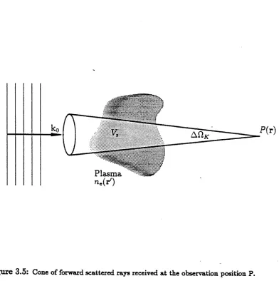
We begin by considering the propagation of an arbitrary incident wave (Fig. 3.1)

through a weakly scattering medium (in this case the plasma). The propagation of

Plasma

Arbitrary Incident Wave

Figure 3.1: Geometry for diffraction from macroscopic plasma irregularities. Note that the form of the incident illumination is not specified.

the incident wave is governed by the relative permittivity Fr, which is a complex

(34)

incident monochromatic held is very high[l], (a;0 ujp + a;« where a;0, ujp and

cJtx are the beam, plasma and electron cyclotron frequencies respectively) then we

may write

t ) — 1 (3.1)

where ne(r, t) is the plasma density and the cutoff density is

n _ *o2

71 cr — . ?

47rre (3.2)

where ka is the incident wavenumber. As long as n^/n^ «C 1 and e* « 1 then the

plasma may be treated as a weakly scattering medium.

Given these restrictions on we investigate the solution to the vector wave

equation for the propagation of electromagnetic waves in an idealized source free

medium. The wave equation can be expressed in terms of the electric displacement

D = eo^E [4]:

( V2 - ^ ) D = - V x v X ( D - e ° E ). (3.3)

Given

E = [E0(r) + E,(r, t)}exp (-jujQt), (3.4)

where Eq is the incident field and Ea is the scattered field and where the first

order solution (setting Ea = 0) is just the equation for free space propagation of

the incident field,

(V 2 -f ^ ) E 0 = 0. (3.5)

This is of course the homogeneous Helmholtz equation for free space propagation

which, in order to distinguish it from the total field (incident and scattered), we

now write as Eo(r, t) = Eo(r) exp (— juot). The general solution of Eqn. 3.5 is a

linear superposition of plane waves. The inhomogeneous wave equation for E , is

given by

— E (3.6)

, — 2 1 0 N_ _ _ ( 7l e \ i O f 71,

^ ‘ w ) - c2 9 ? W - .

where use has been made of the vector identity V x V x = VV. — V 2. Eqn. 3.6

(35)

side is often called the scattering potential or forcing function and is denoted by

f(r, t). The time derivatives can be eliminated using a Fourier representation

together with the low tem perature (nearly monochromatic or quasi-stationary)

approximation. Noting that V .E = 0 in the plasma, the scattering potential

becomes

f(r, t) = — [V (E .V nc) + fc’n .E l . (3.7)

T i e r

Let us consider a single component of the vector wave equation. If we take the

scalar scattering potential to be impulsive,

/ ( r, t) = 8(r - r')5(t - t'), (3.8)

then the inhomogeneous wave equation has the Green’s function solutions :

^ — [*=F i r — 1 /c])

47t I r — r' I (3.9)

In experiments, one usually considers the scattering potential as making no con

tribution to the total field at remote times t —> —oo before the radiation source

is activated. In this case it is appropriate to use the retarded Green’s function

to construct the particular solution for the wave equation [4]. The first order

vector field at the observation point P = P (r) outside the plasma is constructed

from the superposition of wave fields scattered by the collection of point elements

constituting the plasma:

E ( r,t) =

J

d t'f d

= - f dr' ■

g&ilk-

JV. 47T I r — ri I

where the numerator of the integrand is evaluated at the retarded time t‘ = t — q/c.

Substituting Eqn. 3.7 for the scattering potential, and making use of the Fourier

integral representation for n e, we obtain

(3.10)

where

E .( r ,t) = — [ dr' [fcoVE + V '(E .V 'n .)l g{r,r')

n>cx

s(r >r') -e x p (jfe 0| r - r /l) _{47r|r — ril}

(3.11)

(36)

and where the scattering potential has been evaluated at time t by virtue of

the quasi-stationary approximation . Notice the natural appearance of the time

independent Green’s function kernel g. The two terms in the integrand axe dis

cussed by TATARSKI[5] who notes that in the radiaiion zone of the scattered

field (&o I r — r71^> 1), the longitudinally polarized second term ensures that the

scattered field E a is transverse to the direction of propagation.

To show this, an integration by parts may be performed in the radiation zone

giving,

V<7 = jkogq (3.13)

and given the identity,

E = q(q.E ) — q x (q x E), (3-14)

then

E«(r, t) = —47rre exp (—jujot) f d r'n ^ r',* ) [qX (qX E (r'))] #(r, r'). (3.15)

* V*

The classical electron radius is introduced through the relation

re = k%/(Inner). (3.16)

Unfortunately the wave equation, which serves to describe the interaction be

tween the radiation field and the transparent medium, does not yield an exact

solution for the diffracted field in closed form. One approximation valid for scat

tering in the forward direction is where the double cross product in Eqn. 3.14 can

be replaced by —E. This reduces to the scalar diffraction theory, which is exact

for scalar fields such as sound, and is approximate for vector field forward

scattering. This means that the polarization remains unchanged so that we may

introduce the complex field u(r, t) defined as

E (r, £) = E 0u(r, £). (3.17)

The solution to the scattered scalar field is then

.(r , t ) = J v * 7 ( r'> 0 ? (r > r')

(37)

where the scattering potential is

/(r , t) = 47rrene(r, t)u( r) (3.19)

and where

u(r,£) = tio(r) + ug(r,£). (3.20)

Eqn. 3.18 is the solution to the inhomogeneous Helmholtz equation

(V 2 + %)u = / (3.21)

where, for / ( r) = 0, Eqn. 3.20 reduces to the homogeneous Helmholtz equation

(V 2 + k20)uo = 0 (3.22)

valid for free space propagation. Comparing the expression for the scalar scat

tering potential with the vector scattering potential in Eqn. 3.7, it can be seen

that the scalar approximation is valid provided the first term in Eqn. 3.7 can be

neglected. The conditions under which this simplification is valid are discussed in

the literature[6].

3 .1 .2 A p p r o x im a tio n s to t h e S c a tte r e d F ie ld

Unfortunately, the solution (Eqn. 3.18) to the inhomogeneous wave equation

is not obtainable in general as the scattered field appears on both sides of the

equation. A survey of approaches to this problem is given by STROHBEHN[6].

However the simplest approximations most relevant to plasma scattering are when

the scattered field can be expanded in an perturbation series in amplitude or in

phase. The amplitude perturbation series leads to first order to the Bom approx

imation, whilst the first order phase expansion leads to the Rytov approximation.

A detailed analysis of these approximations is presented by GOODMAN[7].

The Bom series is a series expansion of the light amplitude,

u = u0 + ui -f u2 -f- ••• (3.23)

whilst the Rytov series is an expansion of the complex phase,

(38)

It will be shown that the first order Rytov solution, known as the Rytov approx

imation, can be constructed from the first order Bom solution in cases where

the Bom approximation is not valid. Consequently, results derived in the Bom

approximation can be transformed into equivalent expressions valid in the Rytov

approximation. It is known that in many circumstances the Rytov approximation

yields more general solutions to the scattered field than the Bom approxima

tion, not least because the validity of the first order Rytov approximation is not

restricted to the weak scattering limit[6].

Substituting the Bom expansion of Eqn. 3.23 and / ( r , £) of Eqn. 3.19 into the

wave equation 3.21 and talcing only first order terms gives[5],

(V 2 + k*)ui = 47rren euo- (3.25)

Eqn. 3.25 is valid provided

|iti/txo| 1. (3.26)

As a necessary, (though not sufficient) condition for a small scattered component

is th at |A<^>| <C 7r, where A</> ~ rcX0neL is the extra phase shift on propogating

through the plasma, and where L is the thickness of the plasma slab. Then we

arrive at the condition for the Bom approximation to hold,

t t e / t t c r l < AK z/ko (3.27)

where AK z = 27t/ L is the wavenumber uncertainty in the z-direction. Given the

first order approximation to be valid, then

where

u. _[ _{* 7 i ( r ' , % ( r , r ' )}

J —aa

/ i ( r , £) = 47rren e(r,£)uo(r)r(r)

(3.28)

(3.29)

and where r ( r ) is a window function which restricts the volume of integration:

r ( r ) = 1 r £ Vp

(39)

For the Rytov approximation, we write the light amplitude in the form,

u(r,£) = exp[ip(r,t)] (3.31)

where ip is a complex phase. Inserting this expression into Eqn. 3.21 for the

inhomogeneous Helmholtz equation yields the Riccati equation for the complex

phase:

V 2V> + Vtf.VV* + *g(l - — ) = 0. (3.32)

Tl^r

Then, expanding ip out only to first order (ip = ipo + ipi) we obtain,

V V o + Vipo.'Vipo + = 0 (3.33)

for free space propagation and

V V i + 2VipQ.Vipi = 47rrene (3.34)

where we neglect the (’Vipi)2 term, valid provided[6]

(V ^ i)2 < 47rrene = (3.35)

From dimensional arguments, | V ^il ~ KA<p so that the above condition becomes,

n c/ncr (AK z/ K ) 2. This condition is then dependant on the scale size of the in

homogeneity. Note that the condition for the validity of the Rytov approximation

depends on the gradient of the phase and not the absolute phase and th at provided

the phase gradient is not too strong, then the approximation is valid for arbitrarily

large phase shifts. In particular, for forward scattering where \K/ko\ 1 then

the Rytov approximation is generally far superior to the Bom approximation. For

large angle scattering however, \K/ko\ ~ 1, so that the Rytov approximation is

roughly equivalent to the Bom approximation. The attractiveness of the Rytov

approximation is in its ability to accomodate interferometry, where K/ko ~ 0.

Second order correction to ip are discussed by STROHBEHN[6], however we will

ignore higher order approximations which is equivalent to ignoring the effects of

strong refraction. It now remains to identify the nature of the solutions to Eqn.

(40)

It turns out that the solution to f a in Eqn. 3.33 is given by

f a = — (3.36)

uo

where u\ is the solution for the scattered field in the Born approximation in Eqn. 3.25 which can be verified by direct substitution. Hence,

Ar,t) ( = dr'fi(r', t )g( r,r'). (3.37)

As we will not consider higher order corrections to be necessary, we set ipa = f a and u a = u i, and / = / i so that

u (r ,t) = uo(r) exp (T/>,(r, t))

u (r ,t) = uo(r) exp (3-38)

Because of the relative simplicity in evaluating scattered fields for u ay we will develope the theory in the B om approximation, and where necessary, extend the solution to the R ytov approximation by inserting u a and uq into Eqn. 3.36 after

they are determined.

3.1.3 Free Space Propagation

Assum e an incident field propagates in the positive z direction with wavenumber fco. For arbitrary u, the wave field in the plane z = 0 can be decomposed into its incident “angular spectrum” [8]:

A ( k xl ky-, 0) =

JJ

u ( r ',2//;0)ex p [ - j ( k xx' 4- kyy')]dx'dy' (3.39)

= (3-40)

where x' and y ‘ denote spatial coordinates on the incident plane (here taken at

z — 0 and denoted by subscript “i ”), and where (kx, k y ) are wavenumbers on the

incident plane.

Satisfaction of the homogeneous wave equation requires that the Fourier am plitudes A in some plane z be expressed in terms of the angular components A+ on the incident plane by the relation

(41)

where

H{kx,ky]z) = exp \j(k$ - k 2x - k l) 1/2z}. (3.42)

This result is easily obtained upon Fourier transformation of the homogeneous

Helmholtz equation (c.f. Eqn. 3.22). The transfer function H describes free

space propagation and may be regarded as a linear, dispersive, finite bandwidth

spatial filter [9]. Observe th at H is of unit modulus and exhibits phase dispersion

for spatial frequencies less them the bandlimit. This implies that the angular

spectrum is essentially unchanged during propagation in free space so that in

principle one should be able to obtain the amplitudes Ai(kx,ky) at any observer

plane z. Propagation over a distance z introduces only a phase delay between the

spectral amplitudes, depending on the angle of propagation.

The filter transmission is zero for spatial frequencies greater than ko radians

per unit length. In other words, for kl + k* > kg, kz is imaginary and the wave

propagation is evanescent. In the remainder of this chapter we implicitly ignore

the evanescent wave fields as these contributions diminish exponentially away from

the plasma and are insignificant at distances greater than a few wavelengths for

scattering in the forward direction.

One can determine the light amplitude on any plane z from the angular spec

trum at the plane z — 0 by first applying the propagation operator to &y)

and then performing an inverse fourier transform. Doing this we obtain,

u ( x ,y ; z ) =

J

(3-43)

Supposing we have a single plane wave k = (kx, ky, kz) and assuming the radiation

is monochromatic then k = (fcr , ky,(k% — kl — kJ)1/2). Notice that the angular

spectrum of any monochromatic source will then lie on a hemisphere in fourier

space with radius ko and centre (0,0, —ko). This rather innocous result is of central

importance in diffraction tomography and its implications will be discussed in the

next sections where the attractiveness of working in fourier space over the real

(42)

3.1.4 A p p ro x im a tio n s to Free Space P ro p a g a tio n

Several im portant approximations to free space propagation are introduced. Later,

similar approximations will be considered for the scattered field in terms of the

properties of the scatterer. The parabolic approximation in frequency space allows

the free space propagator H to be expressed as,

Hf = exp (jkoz) exp _{- J} + *y (3.44)

where kx and Ky are taken as the displacements from the mean wavenumber which

is assumed to be ko = (0,0, &o). The inverse fourier transform of HF is just the

well known Fresnel kernel hF,

hF{x, y; z) = exp (jkoz) exp[— (x jho 2 + y )].2

j X o z r L 2z

By the fourier convolution theorem and from Eqn. 3.41, we obtain

(3.45)

u(r, t) = Ui* hF

=

JJ

u(x\y'-,0)hF(x - x',y — y ’\ z)<Lx'dy'. (3.46)

However, in relating the amplitude u to the angular spectrum A*, it is instructive

to write the total field in terms of A+. From GOODMAN[8], we may express the

total field u as a fourier transform over Ui with extra quadratic phase factors.

By simply expanding out hF and applying the Fourier convolution theorem we

obtain,

u(r,t) = hF(x,y ;z) (A i * I » ( f c o - , A*j-) (3-47)

z z

where

TF(Kx,Ky-,z) = jXozexp (— j2Trz/zF) (3.48)

and where

zf/(2tt) = (2ko)/(K.2x4- *y). (3.49)

Note th at zF is the Ftesnel length for diffraction from perturbations of wavenumber

(43)

*IY/2-This is a very important result as it indicates not only the precise relationship

between the field and the angular spectrum, but also the likely experimental

degree of difficulty in extracting the spectrum from the measured field. In general,

performing numerical deconvolutions of recorded data in the presence of noise is an

illconditioned process which can generate significant errors, so that various limits

of the diffracted field are sought which provide a simpler relationship between the

field and the angular spectrum.

In the ultra near field, ( z/zj? < 1 ), the second order terms in Hp can be

neglected. The propagated spectrum is then identical, apart from a constant

phase factor, to the initial angular spectrum. All near field techniques rely on

minimal phase dispersion to recover images and angular spectra.

On the other hand, when second order terms can be neglected in the exponent

of hp, (i.e. zA0 (xa 4- y/2)) then IV becomes a simple delta function in which

case,

u(r) = hp( x, y ] z ) Ai(k0- , k 0- ) . (3.50)

z z

This is of coarse the Fraunhofer limit, however, unlike the near field limit where

their is minimal phase dispersion, in the fraunhofer limit, hp behaves as a phase

dispersive filter. The phase curvature in the far field is so strong that relative phase

information between spectral components is lost, and only the power spectrum

may be extracted from the angular spectrum.

Whilst the two most important limits for recovering the angular spectrum

are the ultra near field and the far field, it seems that the phase as well as the

amplitude of the angular spectrum can only be recovered in the near field and

th at it is effectively impossible to recover the spatial relative phase in the far

field due to strong phase dispersion. Thus, far field techniques can only be used

to determine power spectra. An exception to this is when lenses are used, and

where the parabolic approximation still holds on propagation through the optical

(44)

3.1.5 T h e L ens as a F resn el T ran sfo rm in g D evice

It will be shown that the effect of propagation through a lens is to Fresnel trans

form the light amplitude and the parabolic approximation. Given an analytic

expression for u(r) in the absence of a lens and under conditions where the Fres

nel approximation is valid, then the field beyond the lens can be expresses simply

as a coordinate transform on u(r), i.e. (x ,y ;z) —► (x/,y /;z /). This follows nat

urally from the Fresnel transforming properties of lenses and the fact that an

analytic Fresnel transform of Ui(x,y) exist. Various limits of optical systems axe

investigated in terms of the angular spectrum of the incident field. For small angle

scattering in the paraxial approximation and for large enough optical elements,

we may assume apertures to be effectively infinite. Then the optical field through

a series of thin lenses can be obtained from multiple coordinate transformations

of our scalar field u(r).

Suppose we have a light amplitude function uq specified at a distance do in

front of a thin lens, and observe the field u\ at a distance d\ in front of the lens.

Then,

U i(zi,yi;do +

di)

=

JJ

dx0 dyoh^xoô^xi^y^do.dûoixo.yoÔ ) (3.51)

where the lens kernel h i is given by[8]

- 1

W i

x

JJ

<7L(x,y)exp

exp [jko(do + dr)\ exp . ko

'.ko ( l _ 1 _ 1

3 2 U + d, f

x exp

{-*[(2

d„+i ) x+

2d,

+ V

?)

*2+ y )

. ko

(*o + Vo)

(3.52)

and where the integration is over the plane containing the lens with pupil function

This development follows Goodman’s very closely[8], however, where he

proceeds to find approximations to h i in order to derive the lens law for imag

ing, we instead show the correspondence between h i and the Fresnel kernel hp.

Assuming that ctl = 1 then the correspondence is greatly simplified. Performing

Interferometric study of density fluctuations in a tokamak plasma