Preprocessing and Classification of Electrophoresis Gel Images Using Dynamic Time Warping

Int. J. Electrochem. Sci., 8 (2013) 1609 - 1622

International Journal of

ELECTROCHEMICAL

SCIENCE

Preprocessing and Classification of Electrophoresis Gel Images

Using Dynamic Time Warping

Helena Skutkova1, Martin Vitek1,3, Sona Krizkova2, Rene Kizek2, Ivo Provaznik1,3*

1

Department of Biomedical Engineering, Faculty of Electrical Engineering and Communication, Brno University of Technology, Kolejni 2906/4, CZ-616 00 Brno, Czech Republic

2

Department of Chemistry and Biochemistry, Faculty of Agronomy, Mendel University in Brno, Zemedelska 1, CZ-613 00 Brno, Czech Republic

3

International Clinical Research Center – Center of Biomedical Engineering, St. Anne's University Hospital Brno, Brno, Czech Republic

*

E-mail: [email protected]

Received: 31 July 2012 / Accepted: 30 October 2012 / Published: 1 February 2013

The automation of a classification process of electrophoresis gel images is a difficult task. The result highly depends on quality of gel image digitization and on imprecisions in an electrophoretic process. The methodology proposed in the paper helps to remove most of gel image distortions and effectively overcomes the problem of non-uniform electrophoretic process.

Keywords: gel electrophoresis, cluster analysis, taxonomy, dynamic time warping, lane detection, geometric distortion, contrast adjustment, median filtering

1. INTRODUCTION

mostly in a low quality of gel images that makes precise computer processing impossible. The mutual similarity of electrophoresis lanes is often evaluated subjectively in dependence on the number of identical and different bands [6]. The automation of gel images classification requires removal of most significant image distortions such as noise, non-uniform brightness and/or contrast, and geometric disproportion. Most serious distortions are caused by imperfect procedures in the electrophoresis. Suppression or removal of gel image distortions is a known problem that can be solved by a variety of commercial software products [12-14]. Their main disadvantage is a poor adaptation to a specific electrophoretic device and their focus on a specific application.

2. METHODOLOGY

The proposed electrophoretic gel image processing for evaluation of electrophoretic samples similarity consists of five consecutive steps. The gel image is often captured by a low-quality camera. Thus, the first step of the gel image processing is the basic image quality improvement . This step is included in the proposed methodology for two reasons: 1. to ensure the complete automation of the image processing, and 2. to ensure high contrast of grayscale images. The segmentation of the gel image on sample lanes is performed as the second step. The conversion of the gel lane image to the 1-D signal is inseparably related with this step. The signal representation of the gel lane is obtained by median and it can be understood as the non-linear sample filtering. Filtering of samples enhances the useful information contained in the sample (the ratio between the bands and the noise levels of sample background). The sample filtering focuses on each sample separately and eliminates local defects. In addition to the step of median filtering, a special filtering of the sample background was designed in order to remove impurities causing unevenly gray background. Before the last step of cluster analysis used to evaluate the similarity of the samples, the innovative step based on dynamic time warping is integrated. The dynamic time warping adjusts positions of similar bands between two samples, which can be unmatched due to uneven movement of the various samples in the gel.

2.1. Image quality improvement

0 2000 4000 6000

0 0.2 0.4 0.6 0.8 1

0 2000 4000 6000

0 0.2 0.4 0.6 0.8 1

1

1 0

g<1

input

o

u

tp

u

t

1

1 0 _input

o

u

tp

u

t

Relative intensity Relative intensity

Frequ

en

cy

Frequ

en

cy

a) b) c)

+

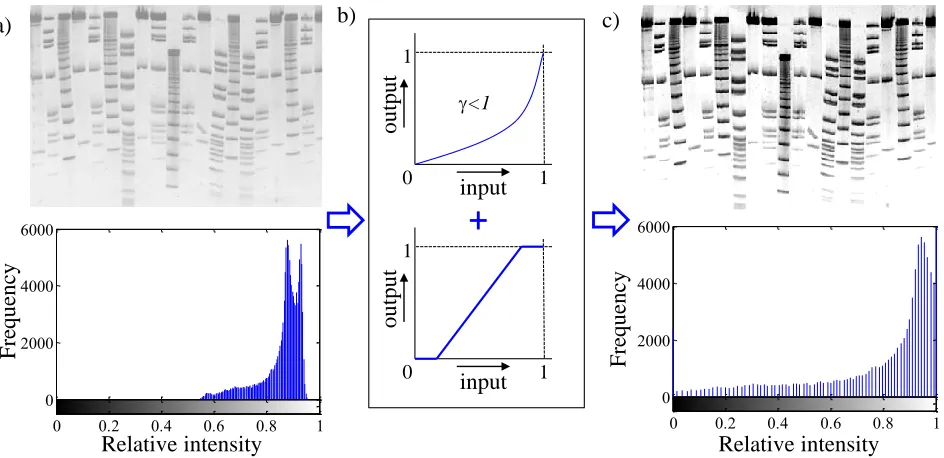
All the other processing steps of gel image analysis require the grayscale image with the white background and the grey level of bands reaching black in the limit. The gray scale can be normalized in the range from 0 to 1 (0 value corresponds to black, 1 corresponds to white) for subsequent computational processing. The grayscale image histogram expresses frequency of the pixels with particular intensity level in relative grayscale range from 0 to 1. The grayscale histogram of the gel image should contain pixels on all levels of the relative grayscale range. A significant increase of the number of pixels is in range from 0.55 to 1, i.e. increased frequency of pixels of white color representing white background. An overexposed gel image has the histogram characteristic tend to 1 (white level), underexposed to 0. The contrast enhancement is realized by transformation function applied to grayscale range of the gel image histogram.

Another useful image enhancement method incorporates gamma correction. The gamma parameter is chosen in dependance on exposition of the image. The overexposed images should be corrected with γ < 1, underexposed image with γ > 1. The range of contrast enhancement for piece-wise linear contrast adjustment is set according to a level of noise in background. Combination of contrast transformations with gamma correction and piece-wise linear contrast adjustment allows the extension of histogram spectrum to entire grayscale range, highlights bands and suppresses background impurities. Figure 1 shows the example of contrast adjustment of an overexposed gel image. The contrast enhancement of the image in panel a) was realized by transformation functions in the panel b). Gamma parameter was experimentally chosen as γ=0.65 and linearly increasing trend of piece-wise linear function was in range between 0.15 and 0.85 of grayscale [19,20].

The choice of parameters of the transformation functions should be manually corrected, because this step is particularly useful to improve the appearance of the result gel image, which is a subjective criterion. The contrast enhancement is not necessary for the similarity analysis of the electrophoretic gel image; the result is changed only slightly and the taxonomy classification only in exceptional cases for very similar samples. This step can be completely skipped or the parameters of the transformation function can be configured based on a density of the histogram for fully automated analysis.

2.2 Automatic detection of lanes

The next step of the electrophoresis image processing is the automatic detection of lanes. Until now, there has been presented a number of approaches to handle the lane detection problem, such as [14,21-23]. These methods are based on a principle called “lane tracking” which lies in tracking of the centre of each lane. The disadvantage of such an approach lies in ignoring of the information from the area outside the central line. In this work, we present a new alternative method for automatic lane detection based on a tracking of lane borders. The result of such an approach is the full segmentation of the lanes. Thus, we can use the information from all pixels of each lane.

the other parameters of the algorithm. The rest of the segmentation process is fully automatic and requires no further human intervention.

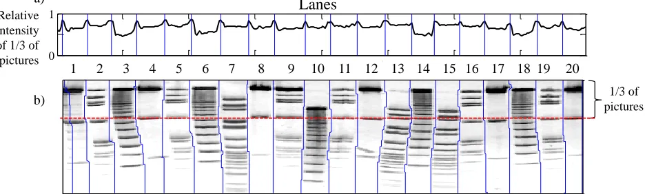
The principle of detection of the first pixel of the lane border is shown in Figure 2a). In the first step, the intensity mean value is calculated for each column of pixels from the upper third of the image. The reason for using only upper third of the image is suppression of the lane shifts in x-axis direction which is greater in the middle and the lower third of the image. The peaks in the obtained 1D signal representation mark the position of the first pixel of each border. The used peak detection algorithm is based on finding local maxima in the signal. It returns only peaks with indices separated by more than the value of variable mpd (minimum peak distance). The variable mpd is calculated as the mean width of the lane multiplied by the constant 0.7. The necessary mean width of the lanes can be easily estimated as the length of the signal divided by the provided number of the lanes in the image.

The next step lies in tracking of the other pixels of each border line. The tracking algorithm starts from the already known positions of the first pixels. These pixels correspond with the uppermost points of blue lines in Figure 2b). In each tracking step, the algorithm compares the intensity values of the three pixels below the current pixel and selects the pixel with the highest intensity (the whitest one). In order to prioritize the most direct path as possible, the value of the middle pixel is a slightly increased by multiplicative constant 1.04. The tracking algorithm stops when reaching the bottom of the gel. The final result of the lane segmentation process is shown in Figure 2b) where the blue lines represent the found lanes boundaries. (The algorithm constants 0.7 and 1.04 were set to achieve best results on the training set of 50 gel images, see example in Figure 7.)

50 100 150 200 250 300 350

0 0.5 1

0 0.5 1

1 2 3 4 5 6 7 8 9 10 11 12 13 14 15 16 17 18 19 20

Relative intensity of 1/3 of

pictures

1/3 of pictures

Lanes

a)

b)

Figure 2.Principle of gel image segmentation using tracking of lane boundaries. a) The detected positions of intensity peaks (blue lines) correspond to the positions of the first pixel of each boarder. b) The final segmented image with marked boundaries of each lane (blue lines).

2.3 Conversion of 2D grayscale image to 1D signal representation

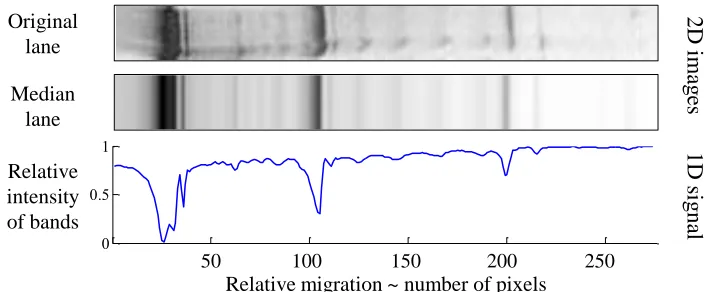
in the image. The important features necessary for subsequent classification are position, thickness and intensity of the bands in each lane. Shifts in the direction of the x-axis and the background noise are the types of image distortion which can be suppressed. In the case of the absence of the shift, the detected boundary lines would be straight. In the case of the presence of the shift, the proposed boundary detection algorithm can trace it. Both emphasize of the features and disorders suppression lies in conversion of 2D lanes to 1D signal representations. The pixels with the same y-axis coordinates within the range of each lane boundaries are replaced by their median value. The possible shift in x-axis direction is eliminated and median also effectively suppresses the image noise. The result of such a conversion can be seen in Figure 3. The figure shows original lane before conversion, the final 1D signal representation and 2D median lane constructed by simple repeating of the 1D signal.

0 0.5 1

Relative migration ~ number of pixels Relative

intensity of bands Original

lane

Median lane

2D imag

es

1D si

g

na

l

50 100 150 200 250

Figure 3.Conversion of a lane image to signal representation using median. a) The original 2D lane after segmentation. b) The 2D lane obtained by median filtering of the original 2D lane. c) Final 1D signal representation of the lane obtained from median values of the original 2D lane. 2.4 Shading correction

0 50 100 150 200 250 300

0 1

0 50 100 150 200 250 300

0 1

Relative migration Relative migration

R

el

at

iv

e

int

ens

it

y

a) b) c)

Figure 4.Correction of shading in electrophoretic lanes. a) The gel image after lane detection and median filtering. b) Upper: The signal of the lane 3 (blue line) with estimation of the signal envelope (red line). Lower: The signal of the lane 3 with removed envelope and normalized values. c) The gel image restored from corrected lane signals.

The estimation of the trend of gray background is realized as finding the signal maxima in a floating window.The window size LW depends on the image resolution and width of the largest band, that the envelope of the background does not follow the course of a signal. The proper window size is twice the size of the largest band and the steps of the floating window with overlap Lo equal one quarter of the window size LW. The window overlap requires the extension of each signal by one length of the window on both sides. The values of extension are the first and last LW values of signal repeated at the beginning and the end. The background envelope estimation is performed separately for each signal (sample). The window parameters were set LW = 20 px and Lo = 5 px for the testing image shown in Figure 4 with the size of 550 × 300 px.

2.5 Adjustment of mutual positions of bands using DTW

The technique called dynamic time warping is was originally used in speech analysis [27]. The same spoken word in the speech of different people has the same meaning (signals are of the nearly same shape), but its timing and offset is specific for each person. The method of dynamic time warping can adapt the timing and offset of such signals [28]. This attribute can be advantageously used for adjustment of bands positions between two gel lanes.

The principle of the DTW is well known in signal processing community [28]. The principle of signals alignment using DTW is shown in the Figure 5. The technique aligns samples values using minimization of the distance between the pairs of samples. Stretching of one or both signals is realized by repeating the selected samples. The criterion for alignment and repetition of samples is determined by the table of accumulated distances (Figure 5 b). The value of accumulated distance is calculated from pairwise distance for each pair of samples in accordance with (1).

0 2 4 6 8 10 12 14 16

0 5 10 15 Time a)

0 2 4 6 8 10 12 14 16

0 5 10 15 Time c)

0 2 4 6 8 10 12 14 16 0 5 10 15 0 2 4 6 8 10 12 14 16 0 5 10 15

0 2 5 7 10 12 9 13 7 12 8 6 4 2 1

0 3 7 11 8 13 9 15 8 12 7 3 i

j i , j

i , j - 1 i - 1 , j - 1

i - 1 , j

b)

Figure 5.General principle of DTW. a) Two original signals of different lengths. b) Determination of the matrix of accumulated distances and optimal path backtracking. Numbers in the first column represent values of the first signal and numbers in the first row represent values of the second signal. The black arrows compose optimal path used for the signal adaptation. The red arrows show the possible directions in each step. c) The resulting signals after DTW (same lengths). ) , ( )] 1 , ( ), , 1 ( ), 1 , 1 ( min[ ) ,

(i j D i j D i j D i j d i j

D       (1)

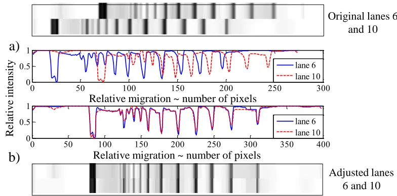
The DTW adapts positions of the same bands but the specificity of each lane is maintained. The principle of adjustment using DTW is shown in the Figure 6. The Figure 6a) shows two similar lanes with different migration speed in image and signal representation. Traditional similarity analysis evaluates only a small amount of mutual similarity in this case. The application of DTW on a signal form of these two signals in Figure 6b) modifies lengths of signals for positional adjustment. The adapted signals were converted again to the image form.

0 50 100 150 200 250 300

0 0.5 1

0 50 100 150 200 250 300 350 400

0 0.5 1

lane 6 lane 10

lane 6 lane 10 Relative migration ~ number of pixels

Relative migration ~ number of pixels

Original lanes 6 and 10

Adjusted lanes 6 and 10

R

el

at

iv

e

int

ens

it

y

a)

b)

Figure 6.Adjustment of band positions in a pair of lanes using DTW. a) Lanes containing similar bands which are not aligned (upper) and signal representation of the lanes (lower). b) Positional adjustment of signal peaks of the lanes (upper) and corresponding image representation of adjusted lanes (lower).

2.6 Similarity analysis of gel lanes

The result of the similarity analysis can be represented by a dendrogram. For gel electrophoresis samples, dendrogram is called a phylogenetic tree [9-11]. The obtained information does not describe only similarity, but also affinity. UPGMA method was used for cluster analysis. Although the method is simple, it is still the most widely used [4-6]. Moreover, testing of cluster analysis techniques is not the subject of this article. The main goal is the extension of common methods by implementing the DTW, new line detection algorithm and the gel image improvement. The dendrogram is reconstructed from pairwise distances determined by (2) as a simple Euclidean distance dxy of two signals X and Y with length k.











 k

i

i i

xy X Y

d

1

2

is not solved. The application of DTW in previous processing step solves both the problems together; therefore the use of correlation coefficient is unnecessary.

If the similarity of samples depends on the mutual offset between two sample lanes, the length of backward way in DTW can be used for weighting of Euclidean distances.

3. RESULTS AND DISCUSSION

The proposed methodology is composed of several innovative steps: the new method of lane detection, conversion of a sample lane to 1D signal and its processing without band detection and application of DTW for signal adjustment. The awareness of their impact to the result is important for their appropriate utilization.

20 40 60 80 100 120 140 160 180 200 220 50

100

150

200

250

300

50 100 150 200 250 300 350 400 450 500

50

100

150

200

250

50 100 150 200 250 300 350 400 450 500

50

100 150

200 250

300 350

50 100 150 200 250 300

50

100

150

200

250

a)

c)

b)

d)

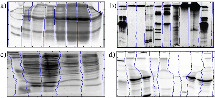
Figure 7.Examples of correct lane detections in four gel images with problematic lane boundaries because lanes overlap each other. a) distortion of protein pattern due to the delay between loading the samples and running the gel, b) bands smearing caused by proteins precipitation during the electrophoresis and uneven proteins concentration in the wells, c) distortion of protein pattern due to delay between samples loading and gel running and high salt concentration in the samples, d) distortion of protein pattern caused by high salts content in the samples, image from http://nu-distance.unl.edu/homer/class/4/mastery/text/geltips.html.

lines with sample lanes and corrects some types of image noise and distortions. The detection works even if the sample lane does not contain any bands (Figure 7d: 6th and 7th lane) and traditional algorithms of sample middle line detection has nothing to detect.

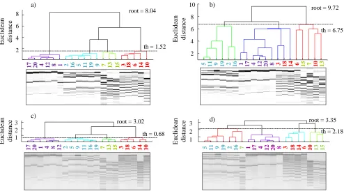
The testing of influence of image and signal pre-processing in combination with DTW was performed on a gel image shown in Figure 1a). The gel image contains four groups of samples which differ in the number of bands and their positions. The division of samples into these groups is color coded in Figure 8. The similarity within groups of samples is relatively clear; the difficult samples to determine are especially the 7th and 10th sample. These sample lanes were degraded by offset (10th sample) and offset with stretching (7th sample). The first group (No. I) is significantly different from the others, because these samples consist of only 3 bands, while the other groups have samples with much more bands. The separation of the first group should be clear from others. The diversification of samples from the remaining three groups is complicated and every small of band positions can cause an error. The criteria for the correct result of similarity analysis are the division into four clusters, the separation of the first group, the classification of distorted samples No. 7 and No. 10 and the threshold of clusters separation. The last criterion takes into account the classification sensitivity; the higher threshold value means worse classification of very similar groups. We set three parameters for an objective evaluation of classification accuracy: th – threshold for clusters separation, root – distance between root and terminal branches, sens – classification sensitivity as a ratio root : th.

1 2 3 4 5 6 7 8 9 10 11 121314 1516 17 181920

I II IV I II IVIII I II IVII I III IVIII II I IV II I Sample

number

Group number

Figure 8.The original gel image with colour coded numbers of samples and groups by mutual similarity.

result was achieved without any adjustment technique in Figure 9c) with DTW utilization. The question is whether to use the image adjustment in combination with DTW or not. The answer lies in mentioned parameters: the clustering threshold and sensitivity. The sensitivity of classification technique with filtration and DTW is sens = 8.04 : 1.52 ≈ 5 : 1 and without filtration sens = 3.02 : 0.68 ≈ 4 : 1. Although the sensitivity of classification without the image filtering is still high, the occurrence of errors will be more possible in the case of more similar sample groups. The proposed filtering technique does not change the result; it only increases the clustering sensitivity.

The remaining dendrograms with reorganized sample lanes in Figure 9b) and 9d) demonstrate the result of classification without using DTW. The cluster analysis alone is not sufficient to classify the damaged samples 7 and 10, even with the help of the image filtering. The internal clusters division is inconsistent, the significantly different group No. I is incorrectly linked with others. Moreover, the sensitivity of clusters separation is significantly below ratio 2:1. The DTW utilization appears more important than the image filtration.

17 20 4 12 8 1 2 16 5 11 19 9 7 13 15 3 18 6 14 10 0 2 4 6 8 8 6 4 2

5 11 9 19 2 16 1 17 4 12 20 8 3 18 14 6 15 7 10 13 2 4 6 8 10 10 8 6 4 2

17 20 4 12 8 1 2 16 5 11 19 9 7 13 15 3 18 6 14 10 0

2 4 6 8

5 11 9 19 2 16 1 17 4 12 20 8 3 18 14 6 15 7 10 13 2

4 6 8 10

17 20 4 12 8 1 2 16 5 11 19 9 7 13 15 3 18 6 14 10 5 11 9 19 2 16 1 17 4 12 20 8 3 18 14 6 15 7 10 13

5 ₁₁ 9 ₁₉ 2 ₁₆ 7 1 ₁₇ 4 _{12 20} 8 3 _{18 14 6 10 13 15}

5 11 9 19 2 16 7 1 17 4 12 20 8 3 18 14 6 10 13 15 1

2 3

5 11 9 19 2 16 7 1 17 4 1220 8 3 18 14 6 10 1315 1 2 3 3 2 1

17 20 1 4 8 12 2 5 9 11 16 19 7 13 15 3 18 6 10 14 1

2 3

1720 1 4 8 12 2 5 9 11 1619 7 13 15 3 18 6 1014 1

2 3

17 20 1 4 8 12 2 5 9 11 16 19 7 13 15 3 18 6 14 10

3 2 1 Euc li de an dist anc e Euc li de an dist anc e Euc li de an dist anc e Euc li de an dist anc e a) b) c) _d)

th = 1.52 root = 8.04

th = 6.75 root = 9.72

th = 0.68 root = 3.02

th = 2.18 root = 3.35

Figure 9.Influence of image and signal pre-processing and DTW utilization on result of sample classification. Classification of gel samples a) with processing and DTW, b) with processing and without DTW, c) without processing and with DTW, d) without pre-processing and DTW. Distance values: th – threshold for clusters separation, root – the length of the tree.

4. CONCLUSIONS

most affordable technology for most (bio)chemical laboratories because of its low purchase and operational costs. However, this fact often corresponds to low quality output which complicates the computer processing of the result gel image. The most common types of outcome degradation are geometric distortion of sample lanes on electrophoretic gel, which occurs already during an electrophoretic process, and the low contrast of the gel image caused by contamination of samples and camera quality. Because the origin of these problems is different and varies, it is appropriate to solve them separately.

Many authors solve a geometric distortion of gel images by modelling their characteristics with subsequent compensation, but a nontrivial distortion is often unpredictable. The presented solution lies in two steps, which separately compensate the distortion in direction of x and y axes regardless of the type and shape of the distortion. The special designed algorithm of the sample lanes detection searches line trend of samples borders and depends only on the changes of gray levels of pixels in the gel image. The trend of line does not have any important characteristic. The correct lane segmentation compensates the geometric distortion in horizontal direction (the lane flexion). The compensation of various relative speeds of different samples on gel in vertical direction is realized by DTW. This step does not solve typical distortions only (as smile affect) but also the individual distortions of each sample. Again, it does not model distortion, because this method adjusts samples to each other, so more precise result is achieved by multiple samples. This fact is related with requirements of similarity analysis, which also needs more samples (10 samples are sufficient).

The elimination efficiency of geometric distortion influence depends on a good visibility of samples in a gel image. The effectiveness of both previous steps increases in dependence on the image quality. The special combination of techniques for image adjustment and signal filtering was proposed for this reason. The contrast adjustment by piecewise linear transform function in combination with the gamma correction improves the lane detection. Filtering of unequal background of each sample improves the position adjustment by DTW and we obtain more accurate evaluation of mutual similarity independent on the background impurities.

The most important fact is that all these steps are adaptive and independent on the used electrophoretic method. It offers universal use and full automaticity of electrophoretic gel image similarity analysis.

ACKNOWLEDGEMENTS

Supported by European Regional Development Fund - Project FNUSA-ICRC (No. CZ.1.05/1.1.00/02.0123) and by the grant project GACR P102/11/1068 NanoBioTECell.

References

1. M. Feizabadi, I. Robertson and D. Cousins, Microbiology, 143 ( Pt 4 (1997) 1461. 2. J. a. Morris, Journal of general microbiology, 76 (1973) 231.

3. S. Krizkova, M. Ryvolova, J. Gumulec, M. Masarik, V. Adam, P. Majzlik, J. Hubalek, I. Provaznik and R. Kizek, Electrophoresis, 32 (2011) 1952.

5. a. Gelsomino, a. C. Keijzer-Wolters, G. Cacco and J. D. van Elsas, Journal of microbiological methods, 38 (1999) 1.

6. F. Amp and E. Miambi, International journal of food microbiology, 60 (2000) 91.

7. M. H. Nicolaisen and N. B. Ramsing, Journal of microbiological methods, 50 (2002) 189. 8. T. Zhang, Biotechnology letters (2000) 399.

9. T. M. LaPara, C. H. Nakatsu, L. Pantea and J. E. Alleman, Applied and environmental microbiology, 66 (2000) 3951.

10. A. E. Murray, J. T. Hollibaugh, C. Orrego, A. E. Murray and J. T. Hollibaugh, Applied and Enviromental microbiology, 62 (1996) 2676.

11. C. R. Woese, Proceedings of the National Academy of Sciences of the United States of America, 97 (2000) 8392.

12. I. Bajla, I. Holländer, S. Fluch, K. Burg and M. Kollár, Computer methods and programs in biomedicine, 77 (2005) 209.

13. J. Pizzonia, BioTechniques, 30 (2001) 1316.

14. R. T. F. Wong, S. Flibotte, R. Corbett, P. Saeedi, S. J. M. Jones, M. a. Marra, J. E. Schein and I. n. Birol, IEEE Transactions on Automation Science and Engineering, 7 (2010) 706.

15. N. Kaabouch, R. R. Schultz and B. B. Singh, 2007 IEEE International Conference on Electro/Information Technology (2007) 577.

16. P. Salas and P. Alvarado, in Conference on Technologies for Sustainable Development TSD2011, 2011, p. 53.

17. X. Ye, C. Suen and M. Cheriet, Vision Iterface (1999) 19.

18. D. C. Rio, M. Ares, G. J. Hannon and T. W. Nilsen, Cold Spring Harbor protocols, 2010 (2010) pdb.prot5444.

19. J. Jan, Medical Image Processing, Reconstruction And Restoration: Concepts And Methods, Taylor & Francis, 2006.

20. C. Dah-Chung and W. Wen-Rong, Medical Imaging, IEEE Transactions on, 17 (1998) 518. 21. A. Machado and M. Campos, in Computer Graphics and Image Processing, 1997. Proceedings., X

Brazilian Symposium on, 1997, p. 140.

22. S. C. Park, I. S. Na, T. H. Han, S. H. Kim and G. S. Lee, Computers and Electronics in Agriculture, 83 (2012) 85.

23. A. Sousa, R. Aguiar, A. Mendonca and A. Campilho, Image Analysis and Recognition, 3212 (2004) 158.

24. S. E. Shadle, D. F. Allen, H. Guo, W. K. Pogozelski, J. S. Bashkin and T. D. Tullius, Nucleic acids research, 25 (1997) 850.

25. Y.-K. Chan, S.-W. Guo, H.-M. Cheng and P.-H. You, 2011 International Conference on Electronics, Communications and Control (ICECC) (2011) 3586.

26. I. Bajla and I. Hollander, Measurement science review, 1 (2001) 5.

27. H. Sakoe and S. Chiba, IEEE Transactions on Acoustics, Speech, and Signal Processing, 26 (1978) 43.