Exploring, exploiting and evolving diversity of aquatic
ecosystem models: a community perspective
Annette B. G. Janssen
.
George B. Arhonditsis
.
Arthur Beusen
.
Karsten Bolding
.
Louise Bruce
.
Jorn Bruggeman
.
Raoul-Marie Couture
.
Andrea S. Downing
.
J. Alex Elliott
.
Marieke A. Frassl
.
Gideon Gal
.
Daan J. Gerla
.
Matthew R. Hipsey
.
Fenjuan Hu
.
Stephen C. Ives
.
Jan H. Janse
.
Erik Jeppesen
.
Klaus D. Jo¨hnk
.
David Kneis
.
Xiangzhen Kong
.
Jan J. Kuiper
.
Moritz K. Lehmann
.
Carsten Lemmen
.
Deniz O
¨ zkundakci
.
Thomas Petzoldt
.
Karsten Rinke
.
Barbara J. Robson
.
Rene´ Sachse
.
Sebastiaan A. Schep
.
Martin Schmid
.
Huub Scholten
.
Sven Teurlincx
.
Dennis Trolle
.
Tineke A. Troost
.
Anne A. Van Dam
.
Luuk P. A. Van Gerven
.
Mariska Weijerman
.
Scott A. Wells
.
Wolf M. Mooij
Received: 3 June 2015 / Accepted: 14 September 2015
!The Author(s) 2015. This article is published with open access at Springerlink.com
Abstract
Here, we present a community perspective
on how to explore, exploit and evolve the diversity in
aquatic ecosystem models. These models play an
important role in understanding the functioning of
aquatic ecosystems, filling in observation gaps and
developing effective strategies for water quality
management. In this spirit, numerous models have
been developed since the 1970s. We set off to explore
model diversity by making an inventory among 42
aquatic ecosystem modellers, by categorizing the
resulting set of models and by analysing them for
diversity. We then focus on how to exploit model
diversity by comparing and combining different
aspects of existing models. Finally, we discuss how
model diversity came about in the past and could
evolve in the future. Throughout our study, we use
Handling Editor: Piet Spaak.Electronic supplementary material The online version of this article (doi:10.1007/s10452-015-9544-1) contains supple-mentary material, which is available to authorized users.
A. B. G. Janssen!J. H. Janse!X. Kong!
J. J. Kuiper!S. Teurlincx!L. P. A. Van Gerven!
W. M. Mooij (&)
Department of Aquatic Ecology, Netherlands Institute of Ecology, PO Box 50, 6700 AB Wageningen,
The Netherlands
e-mail: [email protected]
A. B. G. Janssen!J. J. Kuiper!L. P. A. Van Gerven! M. Weijerman!W. M. Mooij
Department of Aquatic Ecology and Water Quality Management, Wageningen University, PO Box 47, 6700 AA Wageningen, The Netherlands
G. B. Arhonditsis
Ecological Modelling Laboratory, Department of Physical and Environmental Sciences, University of Toronto, Toronto, ON M1C 1A4, Canada
A. Beusen!J. H. Janse
PBL Netherlands Environmental Assessment Agency, PO Box 303, 3720 AH Bilthoven, The Netherlands
K. Bolding!F. Hu!E. Jeppesen!D. Trolle Department of Bioscience and Arctic Centre, Aarhus University, PO Box 314, 8600 Silkeborg, Denmark
K. Bolding!E. Jeppesen!D. Trolle
Sino-Danish Center for Education and Research (SDC), UCAS, Beijing, People’s Republic of China
L. Bruce!M. R. Hipsey
Aquatic Ecodynamics Group, School of Earth and Environment, The University of Western Australia, Perth, WA 6009, Australia
analogies from biodiversity research to analyse and
interpret model diversity. We recommend to make
models publicly available through open-source
poli-cies, to standardize documentation and technical
implementation of models, and to compare models
through ensemble modelling and interdisciplinary
approaches. We end with our perspective on how the
field of aquatic ecosystem modelling might develop in
the next 5–10 years. To strive for clarity and to
improve readability for non-modellers, we include a
glossary.
Keywords
Water quality
!
Ecology
!
Geochemistry
!
Hydrology
!
Hydraulics
!
Hydrodynamics
!
Physical
environment
!
Socio-economics
!
Model availability
!
Standardization
!
Linking
Introduction
The societal niche for aquatic ecosystem models:
developing short-term and long-term management
strategies
Aquatic ecosystems provide a range of ecosystem
services (Finlayson et al.
2005
), in particular by being
sources
and
sinks
for
natural
resources
and
anthropogenic substances. For example, as a source,
they provide water for drinking, irrigation,
hydro-power and industrial processes. Moreover, they
provide many food products. More recently, their
aesthetic and recreational value has been recognized
with associated health benefits. Aquatic ecosystems
also act as a sink for various substances, including
sewage, agricultural run-off, discharge from
impound-ments, industrial waste and thermally polluted water.
Equally important, they provide a critical habitat for
organisms that form an important part of the
biodi-versity. Each of the anthropogenic and natural source
functions puts specific requirements on the quality of
the aquatic ecosystem (Postel and Richter
2003
;
Keeler et al.
2012
). At the same time, these quality
requirements can be hampered by both the source
(through overexploitation) and the sink (through
pollution) functions of the aquatic ecosystem. Aquatic
ecosystem models (hereafter referred to as AEMs)
frequently play a role in quantifying ecosystem
services and developing strategies for water quality
management (Jørgensen
2010
; Mooij et al.
2010
). The
AEMs used for this purpose are often
engineering-oriented based on accepted theory and methodology
for routine applications. Engineering models may be
complex and linked to one another, but components
are always tested. Using projections and scenario
J. Bruggeman
Plymouth Marine Laboratory, Prospect Place, The Hoe, Plymouth PL1 3DH, UK
R.-M. Couture
Norwegian Institute for Water Research, Gaustadalle´en 21, 0349 Oslo, Norway
R.-M. Couture
Ecohydrology Group, Department of Earth and Environmental Sciences, University of Waterloo, 200 University Ave. W, Waterloo, ON N2L 3G1, Canada
A. S. Downing
Stockholm Resilience Centre, Stockholm University, Stockholm, Sweden
J. Alex Elliott
Centre for Ecology and Hydrology, Lancaster, Library Avenue, Bailrigg, Lancashire LA1 4AP, UK
M. A. Frassl!K. Rinke
Department of Lake Research, UFZ, Helmholtz Centre for Environmental Research, Bru¨ckstrasse 3A,
39114 Magdeburg, Germany
G. Gal
Kinneret Limnological Laboratory, IOLR, PO Box 447, 14950 Migdal, Israel
D. J. Gerla
Department of Ecosystem Studies, Royal Netherlands Institute for Sea Research (NIOZ-Yerseke), PO Box 140, 4400 AC Yerseke, The Netherlands
F. Hu
Department of Biology, University of Southern Denmark, Odense M., Denmark
S. C. Ives
Centre for Ecology and Hydrology, Bush Estate, Penicuik, Midlothian EH26 0QB, UK
S. C. Ives
School of GeoSciences, University of Edinburgh, Crew Building, The King’s Buildings, Alexander Crum Brown Road, Edinburgh EH9 3FF, UK
K. D. Jo¨hnk!B. J. Robson CSIRO Land and Water Flagship,
analyses, engineering-oriented AEMs can assess the
various source and sink functions to help optimize and
understand aquatic ecosystem function in terms of
human and conservation needs. For example, AEMs
have been applied as management tools to evaluate the
efficiency of eutrophication mitigation strategies, to
understand oceanic dynamics (e.g. the global carbon
cycle), and to predict biotic responses to climate
change (Arhonditsis and Brett
2004
). AEMs can also
be used for near real-time modelling and forecasting to
facilitate immediate management decisions on, for
instance, the shutdown of drinking water intakes
(Huang et al.
2012
; Silva et al.
2014
) or the suitability
of water for swimming (Ibelings et al.
2003
).
The scientific niche for AEMs: advancement
of theory
A strong scientific motivation for the development of
AEMs is to encapsulate and improve our
understand-ing of aquatic ecosystems. For instance, scientific
AEMs can help to close mass balances of essential
elements such as carbon, nitrogen and phosphorus and
thereby allow quantifying the role of aquatic systems
in national and global carbon and nutrient budgets
(Robson et al.
2008
; Harrison et al.
2012
). Keeping
track of mass balances can also provide help in
answering stoichiometric questions (Giordani et al.
2008
; Li et al.
2014
). Additionally, scientific AEMs
can help untangle the feedbacks between aquatic
biodiversity and aquatic ecosystem functioning
(Bruggeman and Kooijman
2007
), and also achieve
an integrated ecosystem health assessment (Xu et al.
2001
). Yet another timely research topic studied with
models is assessing the resilience of ecosystems to
changes in external forcing arising from nonlinear
functional relationships between ecosystem
compo-nents (Ludwig et al.
1997
; Scheffer et al.
2001
). This
has been done by analysing the strength of various
positive and negative feedback loops in the
socio-ecological system (Van Der Heide et al.
2007
;
Downing et al.
2014
). Such studies generate new
hypotheses that can then be tested in laboratories or in
the field. Models are therefore effective scientific tools
because they allow undertaking ‘virtual experiments’
that would be too expensive or impractical to carry out
in real-world systems (Meyer et al.
2009
).
The methodological niche for AEMs: filling data
gaps and inverse modelling
Another motivation to develop AEMs is to fill gaps in
observations. For instance, some quantities (e.g.
primary production) are measured at high spatial
D. Kneis!T. Petzoldt
Faculty of Environmental Sciences, Institute of Hydrobiology, Technische Universita¨t Dresden, 01062 Dresden, Germany
X. Kong
MOE Laboratory for Earth Surface Processes, College of Urban & Environmental Sciences, Peking University, Beijing 100871, People’s Republic of China
M. K. Lehmann
Environmental Research Institute, School of Science and Engineering, University of Waikato,
Private Bag 3105, Hamilton 3240, New Zealand
C. Lemmen
Institute of Coastal Research, Helmholtz-Zentrum Geesthacht, 21502 Geesthacht, Germany
D. O¨ zkundakci
Department of Ecosystem Research, Leibniz-Institute of Freshwater Ecology and Inland Fisheries,
Mu¨ggelseedamm 310, 12587 Berlin, Germany
R. Sachse
Institute of Earth and Environmental Science, Potsdam University, Karl-Liebknecht-Str. 24, 14476 Potsdam, Germany
S. A. Schep
Witteveen?Bos, PO Box 233, 7400 AE Deventer, The Netherlands
M. Schmid
Surface Waters – Research and Management, Eawag: Swiss Federal Institute of Aquatic Science and Technology, 6047 Kastanienbaum, Switzerland
H. Scholten
Information Technology Group, Wageningen University, Hollandseweg 1, 6706 KN Wageningen, The Netherlands
T. A. Troost
resolution, but at a low temporal resolution and vice
versa. Modelling then allows for interpolation in space
and time such as seen in climatology (Jeffrey et al.
2001
). Other examples include interpolating through
time between satellite images or across space to fill
gaps caused by cloud cover (Hossain et al.
2015
).
Inverse modelling is another application within the
methodological niche for AEMs, in which specific
system parameters or process rates that are difficult to
measure are estimated. In contrast to forward
mod-elling, inverse modelling uses observations to estimate
the processes or factors that created these observations
(Tarantola
2005
). Since inverse modelling in general
lacks a unique solution, it is important to include all a
priori information on model parameters and processes
to reduce the uncertainty on the results (Tarantola
2005
; Jacob
2007
). Methods used for inverse
mod-elling include Bayesian inference, often used with the
Markov chain Monte Carlo technique (Press
2012
;
Gelman et al.
2014
) and Frequentist inference (Press
2012
). Different software packages for
implementa-tion of these methods exist (Ve´zina and Platt
1988
;
Reichert
1994
; Lunn et al.
2000
; Soetaert and Petzoldt
2010
; Van Oevelen et al.
2010
; Doherty
2015
).
Existing diversity in AEMs
Due to numerous potential AEM applications (in an
analogy to biodiversity, we refer to these as ‘model
niches’), scientists began to develop these models in
the 1960s, in tact with the availability of the necessary
computing infrastructure to implement them (e.g.
King and Paulik
1967
). Since then, an array of AEMs
has been developed around the world, with each
development directed by a specific set of questions and
hypotheses.
In
many
cases,
investigators
and
engineers implemented their own models rather than
starting with an existing model. While this practice of
creating one’s ‘own model’ can be criticized because it
bears the inefficiency of ‘reinventing the wheel’
(Mooij et al.
2010
), it has produced a great diversity
in approaches, formulations, complexity and
applica-tions, which can be seen as an advantage. In addition,
the extra investment is often compensated by a more
efficient model application for the issue at hand and a
better model understanding. Furthermore, the
avail-ability of modelling resources through the Internet
provides new opportunities to explore and exploit this
diversity and will most likely affect the evolution of
model diversity in the near future.
A working definition of what constitutes an AEM
This paper aims to present a current perspective on
how we can explore, exploit and evolve the existing
diversity in AEMs as seen by a diverse and
interna-tional community of aquatic scientists (the authors).
We try to reach out to not only the skilled modellers,
but also aquatic ecologists who are inexperienced in
modelling. To make this study feasible, we need a
definition of what constitutes an AEM. Here, we
define an AEM as ‘a formal procedure by which the
impact of external or internal forcing on aquatic
ecosystem state(s) can be estimated’. In most cases,
AEMs cover many processes and are spatially explicit,
but both are not a prerequisite. According to our
definition, a minimal
model that qualitatively
describes the ecosystem response to external forcing
also qualifies as an AEM (Fig.
1
). We exclude models
that focus on one single component of an ecosystem
(e.g. models that only deal with the population
dynamics of a given species), but include models that
zoom in on one part of the ecosystem (e.g. the fish or
macrophyte community) while treating the remainder
of the ecosystem in an aggregated way (typically
through the use of carrying capacities or mortality
rates). Two distinct classes of AEMs exist: those that
formulate a direct mathematical relation between
forcing and state (statistical models), and those that
are formulated in terms of the processes underlying
this relation (process-based models). Statistical
mod-els directly link forcing and state that can be derived
from data with standard statistical techniques. Linking
process-based
models
to
data
involves
less
A. A. Van DamDepartment of Water Science and Engineering, UNESCO-IHE Institute for Water Education, PO Box 3015, 2601 DA Delft, The Netherlands
M. Weijerman
Joint Institute for Marine and Atmospheric Research (JIMAR), University of Hawaii at Manoa, 1000 Pope Road, Marine Science Bldg 312, Honolulu, HI 96822, USA
S. A. Wells
standardized calibration and validation techniques.
The advantage of process-based models is that they
provide insight into the mechanisms underlying
change and recovery. This study is primarily focussed
on the diversity in process-based models, although we
acknowledge the diversity and usefulness of statistical
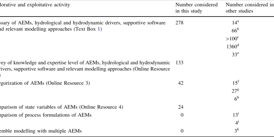
models that directly link forcing and state. AEMs, as
defined here, combine elements from a number of
scientific modelling disciplines (Fig.
2
). In addition to
defining what constitutes an AEM, we developed a
glossary of terminology used in the field of aquatic
ecosystem modelling (given in Text Box
1
). The
purpose of this glossary was to strive for clarity within
the context of this study. This glossary may also be of
help to newcomers in the modelling field. While
working on the glossary, we noted that it is impossible
to make a clear distinction between models (the
mathematical description of a system), their
imple-mentation (e.g. software packages) and their
applica-tions (where model inputs/parameters are adapted to a
specific ecosystem and confronted with data) because
there is great diversity in how these components are
perceived and combined by different modellers.
How this study is structured
We first focus on exploring AEM diversity by
discussing approaches to inventorize, categorize and
document these models and finally present a more
formal analysis of model diversity. To support our
discussion, we compare a number of AEMs,
hydro-logical and hydrodynamic drivers, relevant modelling
approaches and supportive software for model
imple-mentation and model analyses that came about in a
survey among modellers participating the third
AEMON (Aquatic Ecosystem MOdelling Network)
workshop held in February 2015. To put our analysis
in perspective, we compare the number of AEMs,
hydrological and hydrodynamic drivers, relevant
modelling approaches and supportive software for
model implementation and model analyses with
published lists (Table
1
). We cover both marine and
freshwater AEMs, with a bias towards the latter group.
All data can be found in Online Resource 1. It is
remarkable that earlier attempts by Benz et al. (
2001
)
have little overlap with our overview, which shows
that there is a greater diversity than presented here. We
then focus on exploiting diversity and ask several
questions. How can we make use of the full breadth of
expertise captured in existing AEMs, and how can we
easily switch between spatial configurations or
soft-ware packages to run and analyse the models using
package-specific tools? We continue with stressing the
Ec
os
ys
te
m
sta
te
External forcing
a
External forcing
b
External forcing
c
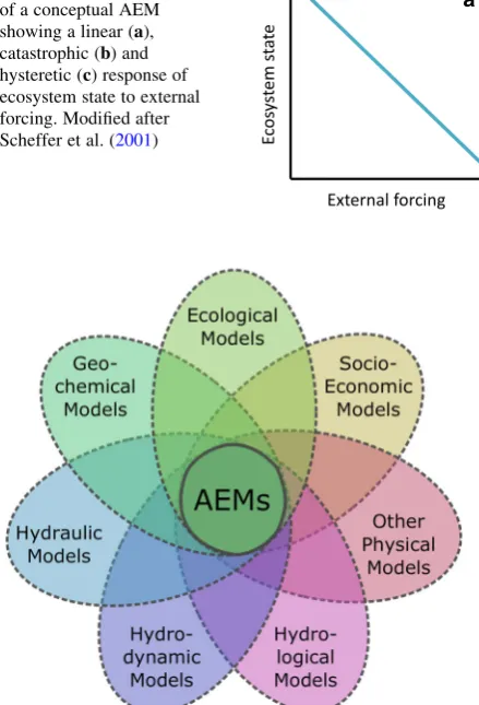
Fig. 1 Example of outputof a conceptual AEM showing a linear (a), catastrophic (b) and hysteretic (c) response of ecosystem state to external forcing. Modified after Scheffer et al. (2001)
[image:5.547.47.267.68.391.2]potential of ensemble modelling, and we end this
section with a discussion on how to exploit the full
range of approaches used in aquatic ecosystem
modelling. In the section on evolving diversity, we
describe the origins of the current diversity in AEMs
and discuss how model diversity could evolve in the
future and how standardization can facilitate this
process. In the final section, we discuss how we can
learn from concepts and techniques in biodiversity
research in our study on model diversity. Finally, we
provide a list of practical recommendations and a
perspective for the field of aquatic ecosystem
mod-elling in the next decade.
Exploring diversity in AEMs
AEMs have been and are being developed
indepen-dently in many places around the world. In this
section, we explore model diversity.
Making an inventory of the diversity in AEMs
An exploratory survey among 42 modellers
partici-pating in the third AEMON workshop 2015 resulted in
133 different models, packages or programming
languages in use in the field of aquatic ecosystem
modelling (data presented in Online Resource 1,
Datasheet 2). We performed a Redundancy Analysis
(RDA, using the methods of Oksanen et al.
2014
) on
39 AEMs from this list (results in Online Resource 2).
This analysis demonstrates that the professional
affiliation and country of origin played an important
role in determining knowledge and usage of models.
The driver behind this could be the research group’s
background, but also the diverging needs that
moti-vated the development of models, such as whether
there are mainly shallow lakes or deep reservoirs in a
specific country. Three approaches seem suited for
developing a more formal and ongoing inventory of
model diversity: (1) lists, (2) wikis and (3) code
repositories. We are not aware of an up-to-date list of
AEMs with a good coverage of the field. Laudable
attempts to list ecological models are UFIS
(Knorren-schild et al.
1996
) and the ECOBAS initiative by
Joachim Benz (
http://www.ecobas.org
, Benz et al.
[image:6.547.61.499.83.302.2]2001
). ECOBAS provides metadata on a wide range of
models,
including
hydrological,
hydrodynamic,
meteorological and ecological models. However, the
website has only rarely been updated since 2009;
Table 1 An overview of the number of AEMs, hydrological and hydrodynamic drivers, supportive software and relevant modelling approaches considered in this and other studiesExplorative and exploitative activity Number considered
in this study
Number considered in other studies
Glossary of AEMs, hydrological and hydrodynamic drivers, supportive software and relevant modelling approaches (Text Box1)
278 14a
66b
[100c
1360d
33e
Survey of knowledge and expertise level of AEMs, hydrological and hydrodynamic drivers, supportive software and relevant modelling approaches (Online Resource 2)
133
Categorization of AEMs (Online Resource 3) 42 15f
27g
6h Comparison of state variables of AEMs (Online Resource 4) 24
Comparison of process formulations of AEMs 0 13i
4j
Ensemble modelling with multiple AEMs 0 3k
a Refsgaard and Henriksen (2004), bhttp://www.mossco.de/doc/acronyms.html, chttp://en.wikipedia.org/wiki (NB: no overview
page of AEMs),dBenz et al. (2001)http://www.ecobas.org(NB: ecological models in general, only 18 overlap with the terms in Text
Box1), ehttps://wiki.csiro.au/display/C2CCOP/Inventory?of?C2C?models, fMooij et al. (2010), gWeijerman et al. (2015), h
updating is a challenge for any top-down initiatives.
An alternative could be an open community-based
approach, such as wikis, where multiple editors
independently contribute information. The obvious
and overwhelmingly successful example of this
approach is Wikipedia (
http://www.wikipedia.org
)
which maintains many lists, for instance of
pro-gramming languages (
http://en.wikipedia.org/wiki/
List_of_programming_languages
).
The
potential
lack of consistency of such community-based lists
seems to be compensated by the scope and
imme-diacy of the information provided and the
commit-ment resulting from the community-based approach.
The third option is code repositories, such as
SourceForge
(
http://sf.net
)
and
GitHub
(
http://
github.com
), which are increasingly popular
plat-forms enabling open-source communities to develop
software and distribute code.
Documenting diversity in AEMs
To preserve and communicate model diversity,
proper documentation of models is crucial. There
is no standard way of documenting AEMs, and
different model developers have different methods
to obtain and save their information. The existing
ODD protocol (overview, design concepts and
details) for individual-based models (Grimm et al.
2006
), the Earth System documentation project
(
http://es-doc.org
)
or
the
TRACE
approach
(TRAnsparent and Comprehensive Ecological
mod-elling documentation) might be adopted by aquatic
ecosystem modellers in the future (Grimm et al.
2014
). Models can be documented through model
homepages, scientific publications or grey literature
reports. Wikipedia is not an option because it has a
strict policy of not being a primary source of
doc-umentation but instead only providing referenced
information. To be useful in the current practice of
scientific research, any type of documentation
should be accessible through the Internet, preferably
with open access. The majority (71 %) of the AEMs
analysed in Online Resource 3 has a website that
provides model documentation. Furthermore, for
86 % of the models, we could identify a primary
publication; however, only three out of 42 AEMs
analysed in Online Resource 3 have a page on
Wikipedia (Ecopath, PCLake and PCDitch).
Categorizing diversity in AEMs
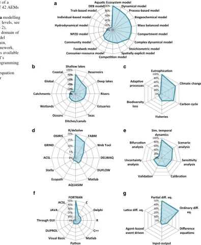
(FABM) (Bruggeman and Bolding
2014
) being the
most used of the 12 modelling frameworks that we
encountered (Fig.
3
d). One can rightfully say that the
field of aquatic ecosystem modelling is quite scattered
when it comes to the use of modelling frameworks.
This notion was one of the incentives for developing
Delft3D-Delwaq (Deltares
2014
), FABM (Bruggeman
and Bolding
2014
) and the Database Approach to
Modelling (DATM) (Mooij et al.
2014
). With 50 %,
FORTRAN is the dominant programming language
for coding AEMs (Fig.
3
f). Next comes C or C
??
(together 26 %), Delphi (15 %) and R (15 %). The
majority of AEMs are implemented as ordinary or
partial differential equations (Fig.
3
g).
100%
Sim. temporal dynamics
Scenario analysis
Sensi!vity analysis
Calibra!on Valida!on
Uncertainty analysis
Bifurca!on analysis
e
0% 20% 40% 60% 80% 100%Eutrophica!on
Climate change
Carbon cycle
Fisheries Biodiversity
loss Adap!ve processes
c
0% 20% 40% 60% 80% 100% Shallow lakes Reservoirs Deep lakes Rivers Estuaries Seas Ditches/canals Oceans Wetlands Catchments Global Coastalb
0% 10% 20% 30% 40% 50%Par!al diff. eq.
Ordinary diff. eq.
Difference equa!ons
Input-output rela!on Agent-based
event driven La!ce diff. eq.
g
0% 20% 40% 60% 80% 100%Aqua!c Ecosystem model Dynamical model
Process-based model Biogeochemical model
Mass balanced model
Compartment model
Complex dynamical model Stoichiometric model Spa!ally explicit model Compe!!on model
Consumer-resource modelFoodweb model Community model
NPZD model Hydrodynamical model Individual-based model
Trait-based modelDEB model
a
0% 5% 10% 15%
20%R/deSolve FABM
Web Tool DELWAQ DUFLOW Matlab AQUASIM Ecopath Stella ACSL GRIND OSIRIS
d
0% 10% 20% 30% 40% 50%FORTRAN CDelphi R C++ Matlab Python Visual Basic DUPROL Through GUI JAVA ACSL
f
Fig. 3 Outcome of acategorization of 42 AEMs on six types of
categorizations:amodelling approach (for all levels, see Online Resource 2), benvironmental domain of the model,cmodel application domain, dmodelling framework, etype of analysis available within the model’s framework,fprogramming language and
[image:8.547.103.499.58.542.2]Analysing diversity in AEMs
Analysing model diversity goes beyond the more
descriptive approach mentioned above. Here, the aim
was to identify whether we are dealing with true
diversity or ‘pseudo-diversity’. Models are often
related to each other. The MyLake model (Saloranta
and Andersen
2007
), for example, has characteristics
that are also found in other lake models such as
DYRESM-CAEDYM
(Hamilton
and
Schladow
1997
), MINLAKE (Riley and Stefan
1988
), PROBE
(Blenckner et al.
2002
) and BELAMO (Omlin et al.
2001
; Mieleitner and Reichert
2006
). We aim for a
more objective and in-depth analysis of a list of AEMs
using a similarity index (for details on the analysis, see
Online Resource 4 and for the data Online Resource 1,
Datasheet 4). One approach is to compare state
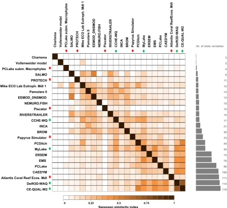
variables between models. We analysed 24 AEMs
for which sufficient information was provided, which
gave in total almost 550 unique state variables. The
minimum number of state variables found in a model
is 2 and the maximum is 118 (Fig.
4
). It should be
noted that in some (especially the larger and general)
models, not all state variables are included
simultane-ously in each model application but rather subsets of
variables are being used. Additionally, some models
have state variables that can be duplicated by changing
their parameters (e.g. cohorts of a species). A Sørensen
similarity analysis (Sørensen
1948
) using the state
variables of 24 models (Online Resource 4) shows that
models become more similar as their complexity
increases. This is an expected result as the chance of
similarities increases with increasing sampling size of
a given pool. However, overall the dissimilarity is
higher than the similarity since more than 80 % of the
models have a similarity index of less than 0.25.
Hence, many models benefit from predecessor models
even though they are still unique with individual
features not found in predecessor models. Most
overlap can be found in general state variables such
as phosphorus, ammonia and a generic group of
phytoplankton or zooplankton. Three groups of
mod-els can be distinguished: general-purpose modmod-els with
a relative high overlap, specialized models with low
overlap and intermediate models with an intermediate
level of overlap (see dendrogram in Online Resource
4). Interestingly, some models are significantly more
dissimilar than would be statistically expected based
on their number of state variables (red downward
arrow, Fig.
4
). This is because these models capture
only a specific non-overlapping part of the aquatic
ecosystem (e.g. the Guam Atlantis Coral Reef
Ecosys-tem Model versus PCLake or CAEDYM). Other
models are more similar than would be expected based
on the number of state variables (upward green arrow);
these models simulate the aquatic ecosystem in a more
general way, such as CCHE and Mylake. A following
step could be to compare the models for their
mathematical process formulations, though this is
beyond the scope of this paper. An educated guess is
that this will reveal an even higher diversity, as endless
combinations can be made with the available process
formulations. For example, Tian (
2006
) counted 13
functions used to describe the effect of light forcing on
phytoplankton growth. Using these light functions in
combination with other functional relations, for
instance, temperature forcing (10 different relations),
zooplankton feeding (20 different relations), prey
feeding (15 different relations) and mortality (8
different relations), lead to hundreds of thousands of
combinations that give different results and are all ‘the
best’, depending on the aim of the model (Gao et al.
2000
).
Exploiting diversity in AEMs
The inventory of the AEMs reveals a great diversity in
model approaches, formulations and applications.
Here, we ask whether and how this diversity could
be exploited.
Exploiting the diversity in disciplines
interdisciplinary teams. In this way, team members are
able to focus on their own area of expertise while the
team as a whole is able to understand the full model.
Statisticians and mathematicians can support
interdis-ciplinary teams with their knowledge on mathematical
formulations and their insight into model uncertainty.
Especially within the scientific niche, understanding
of the model is important since novel ideas need to be
tested and understood. Within the engineering niche,
there is less need to understand each model component
in detail. Indeed, many people drive a car safely
without having a detailed technical background on the
engine’s functionality.
Exploiting the diversity in spatial explicitness
of AEMs
Another way to exploit the diversity in AEMs is by
using the full width of spatial explicitness, which
varies from spatially homogenous (0D) and vertically
Charisma Vollenweidermodel
PCLake
subm.
Macrophytes
SALMO PROTECH Mike
ECO
Lab
Eutroph.
Mdl
1
Pamolare
II
EEMOD_DNSMOD NEMURO.FISH Piscator RIVERSTRAHLER CCHE-WQ INCA BROM Papyrus
Simulator
PCDitch MyLake ERSEM EMS PCLake CAEDYM Atlantis
Coral
ReefEcos.
Mdl
Delft3D-WAQ CE-QUAL-W2 Nr. of state variables
Charisma 2
Vollenweider model 2
PCLake subm. Macrophytes 4
SALMO 8
PROTECH 11
Mike ECO Lab Eutroph. Mdl 1 12
Pamolare II 12
EEMOD_DNSMOD 13
NEMURO.FISH 15
Piscator 15
RIVERSTRAHLER 16
CCHE-WQ 17
INCA 21
BROM 28
Papyrus Simulator 33
PCDitch 44
MyLake 45
ERSEM 75
EMS 76
PCLake 98
CAEDYM 108
Atlantis Coral Reef Ecos. Mdl 111
Delft3D-WAQ 114
CE-QUAL-W2 118
0 0.25 0.5 0.75
Sørensen similarity index 1
Fig. 4 Similarity matrix based on the Sørensen similarity index between the state variables considered in the models.Darker colours mean higher similarity. Models with agreen upward arroware significantly more similar to other models corrected for the maximum number of state variables (p\0.05). Models with a
[image:10.547.49.498.57.467.2]or horizontally structured (1D) to fully 3D. Within
these dimensions, a modeller can additionally
choose between different structured grids (e.g.
Cartesian grid, regular grid and curvilinear grid)
and unstructured grids (e.g. finite elements).
Fol-lowing Occam’s razor, model complexity should be
minimized and only increased if this increases the
predictive performance of the model or its
general-ity/universality (please note that, while mentioned
here in the context of spatial explicitness, Occam’s
razor applies to all aspects of complexity in AEMs).
Therefore, to understand the basics of ecological
processes in a well-mixed system, one should use a
0D model as its dynamics are often easier to
understand. Additionally, 0D models are well suited
for checking the internal consistency of the model
functions. Spatially explicit models, however, are
more realistic, as they account for the spatial
heterogeneity of ecosystems, with the risk of getting
lost in complexity when explaining model
beha-viour. Nonetheless, some research questions cannot
be solved without taking spatial resolution into
account [e.g. population dynamics of fish in Jackson
et al. (
2001
), and spatial distribution of macrophytes
and algae in Janssen et al. (
2014
)]. Recent advances
facilitate the implementation of a model in different
spatial settings. For example, with Delft3D-Delwaq,
FABM and DATM, it is possible to switch between
a 0D, 1D, 2D to 3D implementation of, for instance,
PCLake (Van Gerven et al.
2015
). However, these
frameworks are currently implemented without
accounting for feedbacks between ecology and
hydrodynamics. Interfaces such as OpenMI
(Gre-gersen et al.
2007
) and FABM (Bruggeman and
Bolding
2014
) allow for such coupling and are
designed to overcome the issues that emerge when
integrating ecology and hydrodynamics. Examples
of these issues are the different timescales and
spatial schematization for ecology and
hydrodynam-ics (e.g. Sachse et al.
2014
) and feedbacks between
ecology and hydrodynamics, such as the effects of
water plants on the water flow (e.g. Berger and
Wells
2008
).
Exploiting diversity by having a given AEM
implemented in multiple frameworks
Recent approaches such as DATM (Mooij et al.
2014
),
FABM (Bruggeman and Bolding
2014
) and the open
process library in Delft3D-Delwaq (Deltares
2014
)
make it possible to exploit model implementations in
multiple frameworks without much overhead.
There-fore, a myriad of tools for model analysis (e.g.
sensitivity analysis, calibration, validation,
uncer-tainty analysis, and bifurcation analysis) become
easily available. The redundancy in tools among
frameworks insists modellers to stick to the framework
they are familiar with for most analyses, whereas the
complementarity in tools is tempting to switch to other
frameworks for alternative analyses (Van Gerven et al.
2015
), including the switch between 0D and 3D. In
this way, the strengths of frameworks (including
run-time) can be exploited, and the underlying ecological
question
can
be
approached
from
different
perspectives.
Exploiting diversity in dealing with uncertainty
in AEMs
As a simplification of nature, AEMs suffer from
uncertainty in their outcomes (Beck
1987
; Chatfield
(e.g. Beven
2006
) and bears the risk of overfitting
(Hawkins
2004
). For this reason, a modeller may
choose for the third option where the parameters are
estimated based on calibration data, statistics and a
priori knowledge (e.g. Janse et al.
2010
). In this case, a
realistic range of parameter values is defined, prior to
the parameter estimation by statistics. Thereafter,
using Bayesian statistics, the parameters can be
estimated within the range of realism (Gelman et al.
2014
).
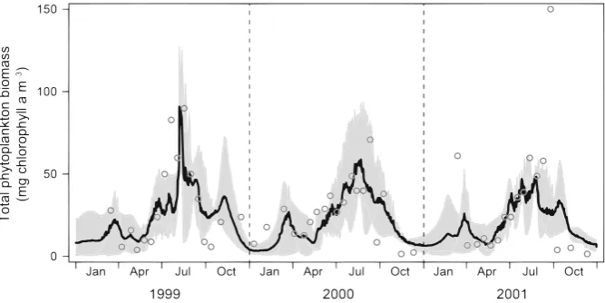
Exploiting diversity by ensemble modelling
with AEMs
One way to deal with the uncertainty is using the
diversity of models in ensemble techniques [e.g.
Ramin et al. (
2012
) or Trolle et al. (
2014
), see Fig.
5
for an example from the latter study]. A variety of
ensemble techniques exists, each duplicating a certain
aspect of the modelling process. In multi-model
ensembles (MMEs), multiple models are applied to a
given problem. Single-model ensembles use different
model inputs (parameters, initial values, boundary
conditions) to exploit the model’s sensitivity (e.g.
Couture et al.
2014
; Gal et al.
2014
or Nielsen et al.
2014
). More ensemble techniques or combinations of
techniques exist including multi-scheme ensembling
(use of different numerical schemes) and
hyper-ensembling (use of multiple physical processes).
Ensemble modelling has become a standard in
meteorological forecasting (e.g. Molteni et al.
1996
)
and climatic forecasting (e.g. IPCC
2014
). There is an
increasing number of applications in hydrology and
hydrodynamics as well (e.g. Stepanenko et al.
2014
;
Thiery et al.
2014
). In aquatic ecosystem modelling,
the use of ensemble techniques is still rare (but see
examples in, for instance, Lenhart et al.
2010
; Ramin
et al.
2012
; Gal et al.
2014
; Nielsen et al.
2014
; Trolle
et al.
2014
). However, the relevance of MME for
ecological modelling is large, as a strictly physically
based description is not practically feasible and a
unified, transferable set of equations is, therefore, not
available. Additionally, we foresee that ensemble
modelling will become common practice because of
(1) the emergence of active communities of aquatic
ecosystem modellers such as AEMON; (2) the
increase in freely available papers, data and model
code; and (3) the development of approaches such as
Delft3D-Delwaq, FABM and DATM. Hence, the
results of decades of individual model niche
develop-ment can now be better utilized (Mooij et al.
2010
;
Trolle et al.
2012
). The comparative list provided in
Online Resource 1 (Datasheet 4) is a useful starting
point of ensemble modelling with AEMs. When using
a model to provide forecasts, MME have two major
advantages over single-model approaches. First, the
ensemble mean may be a better predictor than any of
the sole ensemble members (Trolle et al.
2014
). This is
especially true when an aggregated performance
measure over many diagnostics variables is considered
Fig. 5 Example of a multi-model ensemble (MME). The shaded areashows the full width of predicting outcomes made by different models, theblack lineshows the mean of all models and thecirclesare the observations. Figure modified after Trolle
[image:12.547.107.441.452.619.2](Hagedorn et al.
2005
; Trolle et al.
2014
). Second, the
ensemble spread can serve as a convenient measure of
predictive uncertainty if a spread–skill correlation
exists. Although MMEs are attractive, their limitations
need to be recognized. First, despite ever increasing
computer power, they are time-consuming to put in
place. More importantly, MME-based estimates of
structural uncertainty can only be meaningful if the
models involved differ substantially. Another more
general limitation of ensembles is that the attainable
estimate of uncertainty is inevitably incomplete, for
example due to a limited number of suitable models
and the requirement of each model to have its own set
of—ideally standardized—parameters and initial
val-ues. Ensemble techniques therefore only quantify part
of the total uncertainty in predictions (Krzysztofowicz
1999
). In the context of ecological process-based
modelling though, the integration of multiple models
should not be viewed solely as an approach to improve
our predictive devices, but also as an opportunity to
compare alternative ecological structures, to challenge
existing ecosystem conceptualizations, and to
inte-grate across different (and often conflicting)
para-digms (Ramin et al.
2012
). Future research should also
focus on the refinement of the weighting schemes and
other performance standards to impartially synthesize
the predictions of different models. Several interesting
statistical post-processing methods presented in the
field of ensemble weather forecasting will greatly
benefit our attempts to develop weighting schemes
suitable for the synthesis of multiple ecosystem
models (Wilks
2002
). Other outstanding challenges
involve the development of ground rules for the
features of the calibration and validation domain, the
inclusion of penalties for model complexity that will
allow building forecasts upon parsimonious models,
and performance assessment that does not exclusively
consider model endpoints but also examines the
plausibility of the underlying ecosystem structures,
i.e. biological rates, ecological processes or derived
quantities (Arhonditsis and Brett
2004
).
Exploiting the diversity in fundamentally different
approaches in aquatic ecosystem modelling
Finally, we could exploit the diversity in more
fundamentally different model approaches, for
exam-ple statistical- versus process-based models. The
diversity in model approaches is the product of the
numerous choices that can be made during model
development, pursuing a certain trade-off between
effort, model simplicity, realism, process details,
boundary conditions, forcings and accuracy along
various dimensions such as time and space (e.g.
Weijerman et al.
2015
). For example, minimal models
aim to understand the response curve of ecosystems to
disturbances, but they are generally too simple to
allow for upscaling and process quantification.
Com-plex models on the other hand can describe the cycling
of nutrients through many compartments of an
ecosystem as well as the flow of energy through the
system. Therefore, they often allow for quantitative
scenario evaluations, but their output is difficult to
interpret as it is demanding to decipher the numerous
interactions and feedback loops. More complexity also
can be introduced by individual-based and trait-based
models, which allow the inclusion of evolutionary
processes. Thus, a higher diversity of model
approaches permits addressing a higher number of
different purposes, provided that they are sufficiently
complementary. There is a great value in combining
different modelling approaches, as insights gained by
one model can be useful for the application of another,
and we benefit from the strengths of different model
types (Mooij et al.
2009
). Combining modelling
approaches helps to develop an integrative view on
the functioning of aquatic systems and seems almost
essential for the adaptive management of the source
and sink functions of lake ecosystems, which require
integrated thinking and decision support.
Evolving diversity in AEMs
We have explored and exploited diversity in AEMs.
Before reflecting on possible future evolution of
model diversity, it is interesting first to look back
and see how the existing diversity came about.
A historical perspective on evolving diversity
in AEMs
This sparked the emergence of individual-based
models sensu lato, including dynamic energy budget
models (Kooijman
1993
), structured population
mod-els (De Roos et al.
1992
) and individual-based models
sensu stricto (Mooij and Boersma
1996
), that zoom in
on a particular (group of) species in the ecosystem. In
an opposite direction, minimal dynamical models of
ecosystems zoomed out to detect dominant
nonlinear-ities in ecosystem responses to external forcing
(Scheffer et al.
2001
). Renewed interest in large
ecosystem models occurred in the past decades, not
the least as a result of the increased and distributed
computational power, but this time with the tendency
to link the models with individual-based and
trait-based approaches (DeAngelis and Mooij
2005
) and
compare their behaviour with minimal dynamical
models (Mooij et al.
2009
). In the past, region-specific
questions have led to region-specific models;
how-ever, as a result of current globalization, the need for
widely applicable models and models covering
regional or continental aspects is rapidly increasing.
The growing recognition of the importance
anthro-pogenic stressors on ecosystems and the services
provided by ecosystems asks for coupling of
ecolog-ical models with socio-economics models (e.g.
Down-ing et al.
2014
). This can be realized by using output of
one model as input for the other model, or run-time
exchange of input and output between such models.
The latter method is more complicated and only
becomes necessary when there are strong feedbacks
between ecology and socio-economics.
Arguments for reducing diversity
There are valid arguments why aquatic ecology as a
whole could benefit from streamlining the diversity in
AEMs. First, some formulations have been shown to be
both less accurate and more complex than alternatives
(Tian
2006
). Second, some models are developed to
answer one specific question and thus lose their
functionality once this question has been addressed. It
is likely that this kind of models has a high turnover
rate, but such models could also be incorporated in large
models as the results prove to be relevant. Finally, the
presence of pseudo-diversity is an argument to reduce
the number of models. For example, in climate studies,
it has been shown that the performance of ensemble
models significantly improved when pseudo-diversity
was reduced (Knutti et al.
2013
). Ideally, groups that
work in parallel on similar models should have the
incentives to join efforts, but these incentives are often
not in place. Also at the level of the individual
scientists, there seem to be few, if any, incentives to
give up one’s own model, whereas there are many
incentives to maintain it or even start yet another one.
Only when the incentives that lead to fragmentation are
overcome, or are outweighed by incentives to join
forces, can we expect a healthy consolidation of the
field to take place. Frameworks such as
Delft3D-Delwaq (Deltares
2014
), FABM (Bruggeman and
Bolding
2014
) and DATM (Mooij et al.
2014
) facilitate
this process, but also these frameworks have the risk to
be duplicated, leading to yet another layer of
fragmen-tation. The turnover rate of AEMs is hard to measure
since publications on dropped models are rare, if they
even exist. At the same time, the absence of
publica-tions on a specific model does not necessarily mean that
a model became unused, as engineers, for example,
might use the specific model on a daily basis without
publishing the results. Furthermore, unlike extinct
species that reduce biodiversity, ‘dead’ models can
become ‘alive’ when a need for their existence emerges,
thereby contributing again to model diversity.
Arguments for enlarging diversity
Because the field of aquatic ecosystem modelling can
appear quite fragmented, arguments for enlarging
diversity in AEMs are easily overlooked.
Neverthe-less, there should always be room for good ideas and
new avenues. An interesting example is provided by
minimal dynamical models. When these became
prominent in the shallow lake literature about 25 years
ago, they were met with considerable reservation and
hardly perceived as a step forward. Nowadays, their
ability to illustrate and communicate essential
nonlin-earity in the response of ecosystem (and many other
dynamical systems) is broadly recognized (Scheffer
et al.
2001
). Another emerging approach with many
applications in the aquatic domain is Dynamic Energy
Budgets (DEB) (Kooijman
1993
). The scope of
current DEB models, however, is too limited to be
qualified as ecosystem models as defined in this study.
Arguments for conserving diversity
a loss of useful models and approaches, requiring active
conservation effort by the community at large. Proper
implementation of conservation schemes will help to
prevent the proverbial ‘reinvention of the wheel’
(Mooij et al.
2010
). Additionally, it can help future
model developers to anticipate what models and
formulations worked well and which did not.
Obvi-ously, this learning process is hampered at the lack of
documentation of failures in the scientific literature.
Conserving diversity would thus have a great
educa-tional value and would help understand the ‘genealogy’
of the existing models. Conservation of model diversity
is important for science as well, as science builds on
repetition which only can be complied with when code
is conserved. However, model diversity conservation
has to overcome ‘code rot’, which is the deterioration of
software as a result of the ever evolving modelling
environment, making the software invalid or unusable
(Scherlis
1996
). To prevent code rot, the code should be
maintained. Another option is to conserve models in
their purest mathematical form (e.g. like in the concept
behind DATM, Mooij et al.
2010
).
How to facilitate evolving diversity
One would like to have tools available and mechanisms
in place that would allow diversity to evolve through a
‘natural selection’ of models. Natural selection is an
emergent property of a system in which there is
variation among agents; this variation is transferred to
the offspring of the agents and has an impact on the
survival of the agents. We have shown that there is
ample diversity among AEMs, and there seems to be a
healthy cross-fertilization of ideas leading to continued
development of new versions and models. What may be
hampering ‘natural selection’ among AEMs, however,
are standardized methods to compare model ‘fitness’
within their niche and given the research question they
address. Here, we point specifically to the research
question since models might have a different purpose,
and it only makes sense to compare the fitness of those
models that are able to answer the same research
question. To enhance selection and ‘gene transfer’, easy
model accessibility is necessary in the first place. Easy
accessibility not only includes freely available model
software but also low time costs of, for instance,
learning new modelling code or approaches.
Addition-ally, data availability is very important for the
improve-ment of models (Hipsey et al.
2015
). As long as models
are inaccessible, due to, for example, licence
restric-tions or inappropriate manuals, modellers will most
likely choose the models in use by their colleagues (see
Online Resource 2). These easily accessible models
may not be the best suitable to answer their questions.
Secondly, standard objective assessment criteria to
calibrate and validate models are important (Refsgaard
et al.
2005
; Robson
2014b
). These criteria are different
for each modelling niche, as models that are suitable,
for example, for forecasting of algal blooms require
other criteria than models suitable for biodiversity
assessments. It also implies providing a freely
acces-sible set of data used as calibration or validation data
(meteorology, hydrology, hydrodynamics, nutrient
fluxes, etc.) of the models to be benchmarked. The
application of the models to these common test data
enables a direct comparison without interfering effects
from differences in basin morphometry, hydrology,
meteorology, and so on. The main idea behind this
benchmarking is not to classify models into ‘good’ and
‘bad’ ones, but instead to characterize the dynamic
behaviour and specific abilities of the separate models.
Finally, we would like to point to the importance of the
conservation and maintenance of expertise and
expe-rience for model evolution. Currently, project life
cycles are generally short, and while mobility of people
can help to spread models, the same mobility could lead
to a local loss of expertise (Herrera et al.
2010
; Parise
et al.
2012
).
Discussion
How can biodiversity research help us to interpret
model diversity?
generalists, the majority of the AEMs seem to be
specialists that address the research question that led to
their development but with little application beyond.
This can be attributed to the fact that models are often
locked within frameworks which obstruct
communica-tion and cross-fertilizacommunica-tion between the models (Mooij
et al.
2014
). For the same reason, we could question
whether there is enough competition between the models
to enable survival of the fittest and thus competitive
exclusion. At present, most models seem to have the
fingerprints of the resource group it is developed in, as if
they were species that evolved in their island-specific
supported niche. This has the disadvantage of
reinvent-ing the wheel, but surely has its advantage as well since
the independently evolved models can be used for
comparison as in ensemble modelling.
Recommendations
Our analysis of exploring, exploiting and evolving
diversity in AEMs leads us to three types of
recom-mendations related to (1) availability, (2)
standard-ization and (3) coupling of AEMs.
Availability of AEMs
With respect to the availability of AEMs, it is important
to continue the current trend of open-source policies for
AEM models, tools for analysis and data. This will
increase the transparency of model structure,
assump-tions and approaches. Besides that, there is an urgent
need for a public overview of existing AEMs. This
could be a Wikipedia list, with links to relevant (online)
documentation or similar initiatives. Such a list could
be complemented with an overview of the forces and
niches that created the existing diversity in AEMs.
Once there is an overview of the niches in which models
are designed, the suitability of models for other
applications is better assessed. Documentation of the
available AEMs will create awareness of the full width
of approaches in AEMs to avoid tunnel vision. We
should also actively preserve AEMs to learn from the
past and thereby avoid reinventing the wheel but also to
identify and prevent pseudo-diversity in AEMs.
Standardization of AEM practices
We recommend developing standardization in the
documentation of AEMs [comparable with, e.g. ODD
for IBMs, Grimm et al. (
2006
)], terminology to
categorize AEMs and the methods to analyse AEMs.
Standardization of documentation and terminology is
desirable for the communication on the different
available models. Standardization of methods for
parametrization, comparison, calibration, testing,
structuring, conversion and interpolation in AEMs
will lead to a common practice in model analysis.
Linking AEMs
In our analysis, we compared models by their state
variables, while additional diversity is hidden in the
process formulations. Here, we recommend fulfilling
the next step by comparing models by their process
formulations. Currently, this step is a time-consuming
and difficult task as a result of lack in the availability
of model definitions. Perhaps this step will be possible
in the future due to the emerging linking approaches
such as DATM. And linking has more benefits. We
advocate linking AEMs with models from other
disciplines to answer questions that require a holistic
approach. We recommend running AEMs in more
than one spatial setting to gain more insight into the
effects within the spatial context and suggest running a
given AEM in multiple frameworks to use the full set
of tools for analysis and advice of the user community.
Finally, we recommend ensemble modelling with
AEMs in order to use the best out of multiple models.
For example, statistical- and process-based AEMs
should be used side by side because they have
complementary strengths.
We anticipate that increasing model availability,
standardization of model documentation, and various
forms of linking will lead to an evolving diversity of
AEMs in which the better performing models
out-compete the poorer performing models. Given the
large number of model niches, however, there will
always remain a great diversity in AEMs.
Perspectives
or contribute information through standardized web
interfaces, will gain in importance for the
documenta-tion and distribudocumenta-tion of AEMs. While we recognize the
inherent lack of quality control, we highly value the
ease of access, the community effort and dynamic
nature of this approach (the name ‘wiki’ is derived from
the Hawaiian word for ‘quick’). (2) We recognize
initiatives to develop e-infrastructures for the
imple-mentation of AEMs and other environmental models
where users of different levels of experience share easy
and secure access to models and data according to their
needs. (3) We envision that current trends in the
mandatory storage of scientific data in repositories will
be extended to model code. (4) We envision that online
databases of model parameters will be developed and
become an important resource for the development and
improvement of AEMs. (5) We see a change from the
way consultancy companies earn money with AEMs.
Formerly, their business model was based on copyrights
of model code. Now, we see a switch to a business
model emerging that is based on expertise in applying
open-source models. (6) We hope for a further
integra-tion of the development, analysis and applicaintegra-tion of
AEMs in fundamental research and applied science. It
will be a challenge to develop models of intermediate
complexity that are simple enough to be thoroughly
analysed, yet complex enough to be applicable in
real-life cases. (7) We hope for a better coverage of the
mutual interaction of ecosystem dynamics and
biodi-versity in AEMs. (8) We expect that the domain of
model application (e.g. type of water, climate zone and
stress factors) of AEMs will increase. In the end, this
will allow for global analysis of aquatic ecosystems
exposed to multiple stressors. (9) We envision the
implementation of AEMs in apps that run in a local
context (e.g. using GPS information) on a smartphone
or tablet computer. (10) Finally, we expect that various
forms of ensemble modelling will gain importance.
Through a comparative evaluation of model
perfor-mance, ensemble modelling can contribute to a ‘natural
selection’ of AEMs within their niches that are defined
by questions from society and science.
Text Box 1 Glossary of terms related to aquatic ecosystem modelling. This glossary can also be found in database format in Online Resource 1, Datasheet 1. For each term, an acronym and a description, followed by, in so far known to us, a
Wikipedia page, a homepage or other relevant web pages and one or more key publications is given, using the following style:Term (Acronym):Definition of term (Wikipedia | Web page | Publication)
ACSL (Advanced Continuous Simulation Language): A computer language with user interface and analysis tools for the implementation of sets of ordinary differential equations. (http://en.wikipedia.org/wiki/Advanced_Continuous_Simulation_ Language|http://www.acslx.com|).
ADCIRC (ADvanced CIRCulation Model): A model for storm surge, flooding and larvae drift. (|http://adcirc.org|). AED in FABM (Aquatic EcoDynamics modelling library): A configurable library of biogeochemical model components
including oxygen, nutrients, phytoplankton, zooplankton and sediment implemented in FABM. (|http://aed.see.uwa.edu.au/ research/models/AED,http://sf.net/p/fabm| Bruce et al.2014).
AEM (Aquatic Ecosystem Model): A formal procedure by which the impact of external or internal forcing on aquatic ecosystem states can be estimated. In sometimes used as a synonym for water quality model. (http://en.wikipedia.org/wiki/Aquatic_ ecosystem,http://en.wikipedia.org/wiki/Ecosystem_model,http://en.wikipedia.org/wiki/Water_quality_modelling| | Mooij et al.2010).
AEMON (Aquatic Ecosystem MOdelling Network):A grass roots network of aquatic ecosystem modellers that aims for sharing knowledge, accelerating progress and improving models. (|https://sites.google.com/site/aquaticmodelling|). Agent-based model (): A modelling format used in individual-based models. (http://en.wikipedia.org/wiki/Agent-based_model| |
DeAngelis and Mooij2005).
Algorithmic uncertainty ():A misestimate of the data by the model’s output as result of errors made by the numerical integration method that is used. (http://en.wikipedia.org/wiki/Uncertainty_quantification| |).
AQUASIM (): A modelling framework for the implementation of AEMs in pre-defined compartment types. (|http://www.eawag. ch/en/department/siam/software| Reichert1994).
AQUATOX (): An AEM that predicts the fate of various pollutants. (|http://www.epa.gov/athens/wwqtsc/html/aquatox.html| Park et al.2008).
Text Box 1 continued
Aster2000 (modifiedASTERionella formosamodel): An AEM for reservoirs. (| | The´bault2004).
ATLANTIS (): A flexible, modular modelling framework for developing AEMs that aims to consider all aspects of a marine ecosystem, including biophysical, economic and social aspects. (|http://atlantis.cmar.csiro.au| Fulton et al.2007,2011). BaltWeb (): An application of the model LakeWeb to the Baltic Sea. (| | Ha˚kanson and Gyllenhammar2005).
BELAMO in AQUASIM (Biogeochemical Ecological LAke MOdel in AQUASIM): A biogeochemical and ecological lake model implemented in Aquasim which allows flexible modifications of the differential equations. (| | Reichert1994; Omlin et al.
2001).
BELAMO in R (Biogeochemical Ecological LAke MOdel in R): A biogeochemical and ecological lake model implemented in R which allows flexible modifications of the differential equations. (| | Reichert1994; Omlin et al.2001).
Bifurcation analysis (): A mathematical analysis technique that aims for identifying qualitative shift in model behaviour, e.g. stable versus unstable, in response to internal or external forcing to the model. Extensively used in theoretical ecology, but much less so in the analysis of AEMs, despite its potential to reveal general response curves of the model such as those depicted in Fig.1. (http://en.wikipedia.org/wiki/Catastrophe_theory| | Scheffer et al.2001).
Biogeochemical model (): A model of the chemical, physical, geological and biological processes in an ecosystem. (http://en. wikipedia.org/wiki/Biogeochemistry| |).
BLOOM II (): A phytoplankton community model that uses linear programming, an optimization technique, to calculate the maximum biomass that can be obtained given the available amount of nutrients and constraints on growth and mortality. (| | Los
1991).
BNN-EQR (Bayesian Belief Network model for Ecological Quality Ratio): A statistical model relating Ecological Quality Ratio as defined in the Water Framework Directive in lakes and rivers to abiotic and management factors. (| | Gobeyn2012). Box model (): A representation of a complex system in the form of boxes or reservoirs linked by fluxes. (http://en.wikipedia.org/
wiki/Climate_model#Box_models| |).
BRNS (Biogeochemical Reaction Network Simulator): A simulation environment in which transport processes are interfaced with relevant biogeochemical reactions for sediment diagenesis. (|http://www.geo.uu.nl/Research/Geochemistry/RTM_web/ project1.htm| Aguilera et al.2005).
BROM (Bottom RedOx Model): A water–sediment column model of elemental cycles, redox chemistry and plankton dynamics. (| | Yakushev et al.2014).
C (): A general-purpose procedural programming language. (http://en.wikipedia.org/wiki/C_(programming_language) | |). C11(): A general-purpose object-oriented programming language. (http://en.wikipedia.org/wiki/C%2B%2B| |).
CAEDYM (Computational Aquatic Ecosystem DYnamics Model): A complex ecological and biogeochemical model that can be coupled with the hydrodynamic drivers DYRESM or ELCOM. (|http://www.cwr.uwa.edu.au/software1/models1.php?mdid= 3| Hipsey et al.2006).
Calibration (): - (| | See Model calibration). Cartesian grid (): - (| | See Cubic grid). Catastrophic shift (): - (| | See Regime shift).
CCHE1D-WQ, CCHE2D-WQ, CCHE3D-WQ (Center for Computational Hydroscience and Engineering 1D/2D/3D Water Quality model): A model that simulates water quality processes in river channels, streams, lakes and coastal waters in a 1D, 2D or 3D setting. (|http://www.ncche.olemiss.edu/research/basic/water|).
CE-QUAL-W2 (Corps of Engineers water QUALity model Width averaged 2d): A two-dimensional longitudinal/vertical hydrodynamic and water quality model for reservoirs/lakes, rivers and estuaries that includes full eutrophication modelling state variables including sediment diagenesis, algae, zooplankton, and macrophytes. (|http://www.ce.pdx.edu/w2,http://www. cequalw2wiki.com/Main_Page| Cole and Wells2003).
Charisma (): An individual-based macrophyte community model. (|http://www.projectenaew.wur.nl/charisma| Van Nes et al.
2002b).
CLI (Command Line Interface): A way of controlling a computer or program by entering text messages at a command line. The computer or program responds with text but also with graphical output. (http://en.wikipedia.org/wiki/Command-line_interface| |).
COASTMAB (COASTal MAss Balance model): A dynamic model for coastal water quality based on LakeMab. (| | Ha˚kanson and Eklund2007).
Text Box 1 continued
Code verification ():A substantiation that a model code is in some sense a true representation of a conceptual model within certain specified limits or ranges of application and corresponding ranges of accuracy. (| | Refsgaard and Henriksen2004). COHERENS (COupled Hydrodynamical-Ecological model for REgioNal and Shelf seas): A hydrodynamic driver available
in FABM. (|http://odnature.naturalsciences.be/coherens/about|).
Community model (): A model of closely interacting species within an ecosyst