Filter for detecting and isolating faults for a nonlinear system

(1)

FILTER for DETECTING and ISOLATING FAULTS for NONLINEAR SYSTEM

Leonardo Giovanini and Arkadiusz Dutka

Industrial Control Centre, University of Strathclyde

Graham Hills Building, 50 George St., Glasgow, G1 1QE, United Kingdom E-mail:[email protected]

Abstract: In the paper the problem of detecting and isolating multiple faults for nonlinear systems is considered. A strategy of state filtering is derived in order to detect and isolate multiple faults which appear simultaneously or sequentially in a discrete time nonlinear systems with unknown inputs. For the considered system for which a

fault isolation condition is fulfilled the proposed method can isolate p simultaneous

faults with at least p+q output measurements, where q is the number of unknown inputs

or disturbances. A reduced output residual vector of dimension p+q is generated and the

Keywords: analytical redundancy, dynamic observers, directional residuals, unbiased estimation, state-dependent models.

1. INTRODUCTION

The model-based approach to fault detection and isolation has been subject of intensive research during the last two decades. The procedure of using model information to generate additional signals which are compared with the plant measurements is known as analytical redundancy. Several survey papers on fault detection theory based on analytical redundancy were written by Frank (1990, 1991), Gertler (1988, 1991, 1995) and Patton and Chen (1991).

To enhance the isolability of the faults, the directional properties of the residuals in response to a particular fault has been used. The fault detection filter, a special dynamic observer that generates directional residuals, was first developed at the

beginning of the seventies (Beard, 1971; Jones, 1973).

After that the problem was studied by several authors employing different approaches (Massoumnia, 1986; White and Speyer, 1987; Park and Rizzoni, 1994.a and Liu and Si, 1997).

Park and Rizzoni (1994.b) extended this approach to stochastic linear systems. After an eigenstructure assignment, the remaining degrees of freedom in the design of the filter’s gain are used to minimise the

effect of noises on the output residuals. The obtained fault detection filter can be viewed as a special structure of the Kalman filter with an additional constraint of directionality on the output residuals. The problem of multiple faults was not studied in this work. Later, Keller (1999) developed a fault isolation filter for the linear stochastic systems with multiple faults and unknown inputs. This filter is a particular

form of the Kalman filter that can isolate q faults

given at least q output measurements.

This paper extends the approach proposed by Liu and Si (1997) to non-linear systems with unmeasured inputs and multiple faults using state-dependent coefficient

parametrization. This methodology transfers the nonlinear system into a quasi linear structure. Then, the columns of the fault detectability matrix are assigned as an eigenvectors of the filter’s transition matrix and the remaining freedom of design is used to fix the dynamics of the filter. If there is noise, they are used to minimise its effect on the generated residuals. The proposed strategy can also be applied in the presence of unknown inputs or disturbances robustifying the detection and isolation of multiple faults. The obtained fault isolation filter is very similar to the predictor-corrector structure of the filters for nonlinear systems.

The resulting filter is based on the design of three gains: two to isolate the fault and the remaining one for the

sinc(

i) Laboratory for Signals and Computational Intelligence (http://fich.unl.edu.ar/sinc)

(2)

estimator dynamic. The isolation gains are designed such that one gain is orthogonal to the fault detectability matrix, such that the effect of faults is decoupled, and the other is designed to assign the effect of each fault to only one residual.

The paper is organized as follows. Section 2 introduces the state-dependent model, which will be used to develop the detection and isolation filter. In Section 3 the fault isolation and estimation problem is presented. After that, the observer design is addressed in Section 4. Section 5 gives a numerical example. The results obtained by the proposed estimator is compared with different techniques previously analyzed in the literature. In Section 6 conclusions indications of future research are given.

2. STATE DEPENDENT COEFFICIENT FORM

A wide class of non-linear systems can be

represented by the following non-linear state space model:

(

)

(

)

(

)

( 1) ( ) ( ) ( ),

( ) ( ) .

x k f x k g x k u k y k h x k

+ = +

= (1)

This non-linear state space model can be re-written into the following State Dependent Coefficient (SDC) form with the state dependent matrices:

(

)

(

)

(

)

( 1) ( ) ( ) ( ) ( ),

( ) ( ) ( ).

x k A x k x k B x k u k y k C x k x k

+ = +

= (2)

The state dependent matrices in (2) can be

formulated in an infinite number of ways (Yun et al., 1996). The choice of the proper form of state space matrices depends on a particular case and this may be optimised for the considered model of the non-linear system. As stated in Mracek et al (1996), SDC parametrization may be used to enhance the filter’s

performance, avoid singularities or loss of

observability. The choice of the state dependent

representation should therefore guarantee

observability of the system (2) in linear sense. That

is, the following condition should be fulfilled: ( ) ( )

{

( ) , ( )

}

( ) C x k A x k

x k

∀ is pointwise observable (Mracek

et al, 1998).

For simplicity of the notation, the following notation is introduced for the state-dependent matrices:

(

)

(

)

(

)

, ( ) , , ( ) , , ( ) .

x k x k x k

A =A x k B =B x k C =C x k

3. PROBLEM FORMULATION

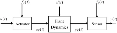
To consider the model–based approach, a mathemati-cal model is developed using a SDC parameterization of the non-linear system. For fault diagnosis and control purposes three separated functional blocks

describe the plant: system, actuator and sensor dynamics (see Fig. 1). Faults are represented by addi-tive signals.

u(t)

fA(t)

y(t) fS(t)

Actuator

uP(t) yR(t)

Plant Dynamics

d(t)

[image:2.612.320.516.105.161.2]

Sensor

Fig. 1. System description.

In this work it is assumed that the dynamics of the system may be non-linear and modelled by the state space model in the SDC form:

, , ,

,

( 1) ( ) ( ) ( ),

( ) ( ),

A A A

A x k A x k x k A

A

R x k A

x k A x k B u k F f k

u k C x k

+ = + +

= (3.a)

, , ,

,

( 1) ( ) ( ) ( ),

( ) ( ),

P

P P

x k P x k P D x k

P

R x k P

x k A x t B u k B d k

y k C x k

+ = + +

= (3.b)

, , ,

,

( 1) ( ) ( ) ( ),

( ) ( ).

S S S

S x k S x k S x k S

S x k S

x k A x k B y k F f k

y k C x k

+ = + +

= (3.c)

The augmented overall system dynamics are given by the following state space model:

), ( )

(

), ( )

( ) ( )

1 (

,

, ,

,

k X C k y

k f F k u B k X A k X

k X

k X k

X k

X =

+ +

= +

(4)

where ( ) ( )T ( )T ( )T T n

A P S

X k =_x k x k x k _ ∈R is the

augmen-ted state vector, ( ) m

y k ∈R is the system output

vector, u

R k

u( )∈ is the control vector,

( ) ( )T ( )T ( )T T p

A S

f k =_f k d k f k _ ∈R i s t h e vector of

disturbances (unmeasured inputs) and fault

magnitu-des, and _, ₁

, ,

n p X k X k p qX k

F =_ f f + _∈R× is the fault /

disturbances distribution matrix. The system matrices are defined by

,

, , , ,

, , ,

, ,

, , ,

,

, ,

0 0

0 ,

0

0 0

0 , 0 0 ,

0 0 0

0 0 .

A x k

P A P

X k x k x k x k

S P S

x k x k x k A A

x k x k

P

X k X k D x k

S x k S

X k x k

A

A B C A

B C A

F B

B F B

F

C C

 

 

=  

 

 

 

 

=_ _ =  

 

  _ _

 

=  

(5)

In the rest of the paper it is assumed:

,

( ) ,

( ) .

X k X k rank C m rank F p q

=

= + (6)

sinc(

(3)

The above assumption must be fulfilled for the considered operating state space. This assumption is fulfilled in most of chemical processes, mechanical and aerospace systems.

Now, we extend the definitions of fault detectability index and matrix given by Liu and Si (1997).

Definition 1: The state-depend system (4) has fault

detectability indexes ρX,k= {ρ1X,k,…,ρpX,k} at the

current state X(k) if

1

, ,

1

min : 0 1, 2,

o

iX k X k X k l iX k o

l

o C A o

ρ − − −

=

 

= _ ≠ = _



∏

f 

…

where

, , 1 ,

,

, . m

X k X k X k m

X k l l

A A A l m

A

I l m

− − − ≤  =  > 

∏

…

Assuming that the system (4) has finite detectability

indexes, the fault detectability matrix DX,k is defined as

, ,

X,k X,k X k

D =C Ξ (7)

where

1

1 1

, , 1 , , ,

1 1

. p

p

X k X k l X k X k l pX k

l l A A ρ ρ ρ ρ − − − − + − = =  

Ξ =  

 



∏

f

∏

f 

(8)

Now, grouping and ordering the columns of ΞX,k and

the elements of f(k) by the detectability index, the

detectability matrix can be written as follows

1

1 1 ,

1

,

( 1) ( 1) ( ) ,

s

X,k X,k X k l sX,k s

l

T T

S A

k φ k φ k s

−

− −

=

 

Ξ _{= } _

 

 

Φ − =_ − − _

∏

F F

(9) where

{

}

[

]

, , ,

max 1, 2, , ,

: , 1 2 ...,

( ) ( ) ( ) .

l l l

i

lX k mX k nX k m n

T

l m n

s i p

m n, ρ ρ l , , s

k l f k l f k l

ρ ρ ρ

ρ φ − − − = = = ≠ = = − = − −    

F f f

…

Due to the additive effects of faults occurring at time

instant r (with k> r +s), the system output y(k)can

be computed from the last state X(k−1)and past

inputs (control actions, disturbances and faults) as follows

, , , ,

, ,

( ) ( 1) ( 1)

( 1).

X k X k X k X k

X k X k

y k C A X k C B u k

C F f k

= − + −

+ − (10)

By defining the state X~(k) without the effect of the

last disturbance which can be seen on the output may be written as follows

), 1 ( ) 1 ( ) ( ~ , , − + −

=A X k B u k

k

X Xk uXk

the system output is given by

, , ,

( ) _{X k} ( ) _{X k} _{X k} ( 1)

y k =C X k +C Ξ Φ −k ₍₁₂₎

Observe that the first term is the current state, X~(k),

without the effect of the faults and disturbances. Note the fact that the effect of disturbances and faults from the states is isolated here. In the future this result will be used to build an observer that can detect and isolate the effect of faults and disturbances from the outputs.

4. THE FAULT ISOLATION FILTER DESIGN

Consider the dynamic observer given by the following equation: ) ( ˆ ) ( ˆ ), ( ) ( ) ( ˆ ) 1 ( ˆ , , , , k X C k y k q K k u B k X A k X k X k X k X k X = + + = + (11)

where Xˆ(k) and yˆ(k) are the state and output

estimate vectors. Employing the equation, the output residual q(k) is given by

, , ,

ˆ

( ) ( ) ( ),

( ) ( 1),

X k X k X k

q k y k y k

C e k C k

= −

= + Ξ Φ − (12)

where e(k) is the estimation error

ˆ

( ) ( ) ( ).

e k =X k −X k

Observe that the residual q(k) has two components: i)

the estimation error due to state errors e(k), without

the effect of disturbances and faults, and ii) the effect of the past disturbances and faults over the system outputs. The effect of this term is that the estimation is biased in a way that could lead to the divergence of the estimated states. To solve this problem we

introduce two matrix coefficients ΤX,k and ΣX,k

(Kitanidis, 1987; Nagpal et al., 1987). Then, the residual is represented using two variables, which are given by the following expression

( ).

) 1 ( ˆ ) ( ˆ , , k q k k q k X k X       Τ Σ =       − δ (13)

Replacing the residual q(k), the previous equation

could be rewritten as

, , , , ,

ˆ( ) ( ) ( 1),

ˆ( 1) ( ) ( 1).

X k X k X k X k X k X k X k X k X k X k

q k C e k C k

k C e k C k

δ

= Σ + Σ Ξ Φ −

− = Τ + Τ Ξ Φ −

where p q

R k₋₁₎_∈ + (

ˆ

δ are the residuals associated to

faults and ( )

) (

ˆ m p q

R k

q ∈ − + are the residuals decoupled

from the faults and disturbances. To obtain an

sinc(

(4)

unbiased estimation we have to remove the effect of the disturbances and faults from the estimation error.

Thus, the matrices ΤX , k and ΣX , k must satisfy

( )

, , ,

0 ,

. m p q X k X k X k

p q p q

X k X k X k

C R

C I R

− +

+ × +

Σ Ξ = ∈

Τ Ξ = ∈ (14)

The matrices ΤX , k and ΣX , k are given by

(

)

(

)

, , , , , , , , ,

X k X k X k

X k m X k X k X k

C

I C

υ

+

Τ = Ξ

Σ = − Ξ Τ

where υ is a vector that guarantees that the first

m-(p + q) elements are full rank. Under this design

condition, the components of the residual q(k) are

given by ). 1 ( ) ( ) 1 ( ˆ ), ( ) ( ˆ , , , , − + Τ = − Σ = k k e C k k e C k q k X k X k X k X δ δ (15)

Then, the fault isolation filter is given by

[

]

,

, , , ,

, ,

,

ˆ₍ ₁₎ ˆ_{( )} _{( )} _{( ),}

ˆ

ˆ( ) ( ),

ˆ( 1) ( ).

X k

X k X k X k X k

X k

X k A X k B u k K W q k

y k C X k

k q k

δ

Σ + = + +

Τ =

− = Τ

 

 

 

(16)

where KX k, is the filter gain and WX,k is the matrix

that propagates the effect of disturbances and faults

. X,k X,k X,k

W =A Ξ (17)

Note that the feedback action is only applied toqˆ(k),

whileδˆ(k−1) is updated in a feedforward way

through WX,k. Therefore, if there is any mismatch the

estimation of the faults δˆ(k−1) will exhibit an offset

error.

The fault isolation filter (16) can be re-written as follows

, ,

,

ˆ₍ ₁₎ ˆ_{( )} _{( )} _{( ),}

ˆ

ˆ( ) ( ),

ˆ( 1) ( ),

X k X,k X k

X k X k

X k A X k B u k K y k y k C X k

k q k

η

+ = + +

= − = Τ

(18)

where

, ,

,

X,k X,k X,k X,k X,k X k X,k X,k

X,k X,k X,k X,k X,k

A A W C K C

K K W

= − Τ − Τ

= Σ + Τ

(19)

The next step to design the filter is to compute the

filter gain KX,k. If the signal/noise ratio is high

(SNR>>1), KX,k can be designed by pole placement.

First, the eigenvalues of the observer are

placed 0

~ ~

A

AX,k = then using (19) KX,k is given by

(

C

)

(

A A W C

)

k

KXk = ΤX,k X,k − X,k− X,kΤX,k X,k ∀

− 0 1 , ~ .

The proposed filter can be easily extended to the

stochastic case. In this case, the filter gain KX,k must

be calculated like in the stochastic case (Mracek et al.,

1996). Therefore, the gain KX,k is obtained from the

solution of the Ricatti equation

(

) (

)

(

)

1 , , , , , , , ,

, , , , 1 , , , , , , , , , , , . T k X k X k X k X k k X k X k X k X k

T T X k X k X k X k

T T T

X k X k K X k X k X k X k k X k X k X k X k

P A K C P A K C

K Q K R

K A P C C P C Q

+

−

= − Σ − Σ

+ Σ Σ +

= Σ Σ Σ + Σ Σ

5. SIMULATIONS

As the numerical example the following discrete-time system is considered:

2, ,

4,

0.1 0 0 0

0.9 0.2 0.1 0 0

0 0.2 0.2 0

0.3 0 0 0.3 sin( )

k X k k x A x    ₊    =    _⋅      , , ,

1 1 0.4

0 0 0 1

0 0 0

, 0 0 0.1 0 ,

0 0 1

0 0.8 0 0

0 0 0

X k X k X k

B C F

                = =_ _ =                

The input signal is given as:

( ) 1 0.4 sin

100

k u k = + _ ⋅π_

 

The fault magnitudes are:

1 0 50 ( ) 0.1 50 for k f k for k <  =  _≥ 

2( ) 0.05 sin 10

k f k = ⋅ _ _

 

The state-dependent matrix A_{X k}_, is updated using the

state estimate obtained from the filter. In Fig. 2 the directional residuals obtained using presented filter are plotted.

In Fig. 3 the innovation

q k

ˆ( )

of the non-linear fault

detection filter is shown. The state estimate obtained from the filter, which is used for the model update, may be influenced by the faults and the estimation time delay. It may be noticed that accuracy of estimation is limited by the model mismatch which results from the inaccuracy of the state estimation. In some cases the non-linearity of the system depends on the state which may be measured directly. This

sinc(

(5)

would remove the model mismatch and lead to a very accurate result.

0 50 100 150 200 250 300 350 400

-0.06 -0.04 -0.02 0 0.02 0.04 0.06 0.08 0.1 0.12 0.14

Fig. 2: Directional residuals

δ

ˆ

- non-linear filter fault detection filter

0 50 100 150 200 250 300 350 400

-0.005 0 0.005 0.01 0.015 0.02 0.025

Fig. 3 Innovation

q k

ˆ( )

of the non-linear fault detection filter

The results for non-linear filter may be compared

with those obtained from the linear filter. The A

matrix for such filter is calculated using the steady state of the non-linear system without faults and with

( ) 1

u k = which is the average value of control signal.

The results are shown in Fig. 4.

0 50 100 150 200 250 300 350 400

-0.1 0 0.1 0.2 0.3 0.4 0.5 0.6

Fig. 4: Directional residuals

δ

ˆ

- linear fault detection filter

The superiority of the non-linear filter may be noticed here and the main reason for that is the fact

that more accurate model was used. The model mismatch present in the non-linear filter due to state estimation bias is not as high as in case, when the fixed linear model is used for estimation with non-linear object. Finally the innovation sequences of standard State-Dependent non-linear filter (Mracek et. al. 1996) are plotted in Fig. 5

0 50 100 150 200 250 300 350 400

-0.05 0 0.05 0.1 0.15 0.2 0.25 0.3 0.35 0.4

Fig. 5: Innovation sequence of the non-linear Kalman filter

6. CONCLUSIONS

This paper has presented a new fault isolation filter for discrete-time non-linear systems. The filter is based on the parametrization of the nonlinear system which transfers the problem to a linear structure with state-dependent coefficients. The accuracy of the estimation is limited by the model mismatch which results from the state estimation errors. For some systems the non-linearity depends on the state which may be measured directly and the model mismatch may be removed and accurate result obtained. The more accurate state estimation techniques minimising the effect of model mismatch will be subject of further research.

The fault isolation filter can isolate p faults and q

unmeasured inputs/disturbances with at least p+q

output measurements. Each element of the residuals

vector of dimension p+q is decoupled from other

faults (or disturbances). This component may be associated with only one fault and statistical tests may be used for detection, isolation and estimation of

multiple faults appearing simultaneously or

sequentially in the system.

ACKNOWLEDGEMENTS

We are grateful for the support of the Engineering and Physical Science Research Council

(EPSRC) grant Industrial Non-linear Control and

Applications GR/R04683/01.

sinc(

[image:5.612.104.283.90.230.2] [image:5.612.324.504.142.279.2] [image:5.612.102.283.267.404.2] [image:5.612.101.288.520.683.2]

(6)

REFERENCES

Beard, R. (1971), Failure accommodation in linear

systems through self-reorganization, Ph.D.

dissertation, Cambridge, Massachusetts.

Frank, P. (1990). “Fault diagnosis in dynamic systems using analytical and knowledge based redundancy - a survey and some new results”,

Automatica, Vol.26, pp.459-474.

Frank, P. (1991). “Enhancement of robustness in

observer-based fault detection”, IFAC/Ii14ACS

Safeprocess Conference, Baden-Baden, Germany, pp.275-287.

Gertler, J. (1988). “Survey of model-based failure detection and isolation in complex plants”, IEEE

Control Systems magazine, Vol. 8, pp.3-11.

Gertler, J. (1991). “Analytical redundancy methods

in fault detection and isolation”, IFAC/IMACS

Safeprocess Conference, Baden-Baden, Germany, pp. 9-21.

Gertler, J. (1995). “Generating directional residuals

with dynamic parity relations”, Automatica, Vol.

31, pp. 627-635.

Jones, H. L. (1973). “Failure detection in linear

systems”, PhD dissertation, Cambridge,

Massachusetts.

Keller, J.-Y. (1999). Fault isolation filter design for

linear stochastic systems, Automatica, Vol. 35,

pp. 1701-1706.

Kitanidis, P.K. (1987). “Unbiased minimum variance

linear state estimation”, Automatica, Vol. 23, pp.

775-778.

Liu, B. and J. Si (1997). “Fault isolation filter design

for time-invariant systems”, IEEE Trans. Autom.

Control, Vol. 21, pp. 704-707.

Massoumnia, M. (1986). “A geometric approach to

the synthesis of failure detection filters”, IEEE

Trans. on Automatic Control, Vol. 31, pp.

839-846.

Mracek, C., Cloutier, J. and C. D'Souza (1996). “A

new technique for nonlinear estimation”,

Proceedings of the 1996 IEEE International Conference on Control Applications, Dearborn, pp. 338-343.

Mracek, C. P., Cloutier, J. R. (1998), Control designs for the nonlinear benchmark problem via the

state-dependent Riccati equation method, Int. J.

of Robust and Nonlinear Control, Vol. 8, pp.

401-433.

Nagpal, K., R. Helmick and C. Sims (1987). “Reduced-order estimation: Part 1. Filtering”, Int.

J. Control, Vol. 45, pp.1867-1888.

Park, J. and G. Rizzoni (1994). “A new interpretation

of the fault detection filter: Part 1”, Int. J.

Control, Vol. 60, pp. 767-787.

Park, J. and G. Rizzoni (1994). “A new interpretation of the fault detection filter: Part 2“, Int. J Control, Vol. 60, pp, 1339-1351.

Patton, R and J Chen (1991) “A review of parity

space approaches for fault diagnosis”,

IFAC/IMACS Safeprocess Conference,

Baden-Baden, Germany, pp. 65-81.

White, J. E. and J. L. Speyer (1987). “Detection filter

desire: Spectral theory and algorithms”, IEEE

Trans. Autom. Control, Vol. .32, pp. 593-603.

Yun Huang and Wei-Min Lu (1996). “Nonlinear optimal control: Alternatives to Hamilton-Jacobi

Equation”, Proceedings of 35th Conference on

Decision and Control, Kobe-Japan, pp. 3942-3947.

sinc(