Multi-Objective Resource Selection in Distributed Information
Retrieval
Shengli Wu and Fabio Crestani∗ Department of Computer and Information Sciences
University of Strathclyde Glasgow G1 1XH, Scotland, UK Email: <shengli, fabioc>@cs.strath.ac.uk
Abstract
In a Distributed Information Re-trieval system, a user submits a query to a broker, which determines how to yield a given number of doc-uments from all possible resource servers. In this paper, we propose a multi-objective model for this re-source selection task. In this model, four aspects are considered simulta-neously in the choice of the resource: document’s relevance to the given query, time, monetary cost, and sim-ilarity between resources. An opti-mized solution is achieved by com-paring the performances of all pos-sible candidates. Some variations of the basic model are also given, which improve the basic model’s efficiency.
Keywords: information retrieval, resource selection, distributed digi-tal libraries.
1 Resource Selection in Distributed Information Retrieval
With the rapid growth of information avail-able via Internet, a huge number of resources are available to users. However, the user often finds it difficult to select the most appropri-ate resource, given an information need. Dis-tributed Information Retrieval (DIR) can help
∗
Author to whom correspondence should be sent.
in this task by automating theresource selec-tion process and making it transparent to the user [8].
In the Information Retrieval and Database research communities, much of the atten-tion has been devoted to select those re-sources which could provide the largest num-ber of relevant documents. Some heuristic methods have been proposed, for example, in [2, 5, 11, 9, 1, 6].
Another important factor in resource selec-tion in DIR is the chance of gettingdocument duplicates. The issue of dealing with docu-ments duplication in different resources has been approached by several researchers, for example in [7, 4]. It is obvious, that if many duplicates are present in the fused retrieval set, the user will waste money and time and even if the service was free, it would still be annoying for the user to be presented with several identical documents. To prevent this from happening, two things could be done at two different stages by DIR systems. Firstly , at resource selection stage, a distinctive policy can be used to select those resources which are more likely to provide document duplicates for a given query. Secondly, at data fusion stage, duplication (totally or partially) can be checked out and redundant documents can be eliminated. While for duplicate detection, processing documents at data fusion stage is an indispensable complex process, since doc-uments could not be identical but similar, so-phisticated resource selection policy could al-leviate the problem and help improving the effectiveness and efficiency of the whole sys-tem. Therefore, a two-stage process solution is a sensible way. In this paper we will not deal with document processing for duplicate detection, but we will introduce in the re-source selection model a factor that will take into account the chance of getting document duplicates.
We argue that multi-objective optimization could provide an appropriate solution to deal with the above problems. In the following of this paper, we will present a multi-objective resource selection model for DIR. The model considers four aspects of resources: relevance of the documents to the given query, time, monetary cost, and chance of getting docu-ment duplicates. The rest of the paper is orga-nized as follows. Section 2 presents the frame-work and the basic resource selection model. Section 3 provides a general solution to the above model. Section 4 briefly discusses ex-tensions to the basic model. Section 5 con-cludes the paper.
2 A Basic Resource Selection Model
Assumption 1. In every local resource, the doc-uments retrieved for any query are ranked in a descending order of estimated relevance.
We think this is an acceptable assumption since it is quite commonly met by most of today’s Web search engines, Digital Library systems, and Information Retrieval systems.
Assumption 2. For any query, the user always specify a number n, instructing to the DIR sys-tem to retrieve the top n estimated relevant documents.
Suppose we have m resources for considera-tion, D denotes the set of resources we have, and D(i) (1 ≤ i ≤ m) denotes the i-th re-source among them. In the following, all the parameters are related to the result of a given query Q. Doc(i) denotes the re-sult set we get from D(i) with respect to
Q. N(i) denotes the number of documents in
D(i). Doc(i, j) denotes thej-th document in
Doc(i), andR(i, j) denotes the relevance esti-mate forDoc(i, j). According to Assumption 1, all retrieved documents appear in descend-ing order of estimated relevance. Therefore, for any 1≤j≤N(i)−1,R(i, j)≥R(i, j+ 1).
Tall(i, j) denotes the time spent to retrieve the
first j documents inDoc(i), while C(i, j) de-notes the charge or monetary cost to be payed forDoc(i, j).
Assumption 3. For every local resource D(i), and every documentD(i, j)returned from it for a given query, the estimated relevance R(i, j)
has been normalized so that 0 ≤ R(i, j) ≤ 1
always holds.
It is also useful to consider the following mea-sures:
Avg T(i, j) = Tall(i, j)
j
Avg C(i, j) = 1
j j
X
k=1
C(i, k)
Avg R(i, j) = 1
j j
X
k=1
which denote the average time, the average charge, and the average relevance of the first
j (1≤ j ≤ N) documents in Doc(i), respec-tively.
Among them, Avg T(i, j) and Avg C(i, j) need further normalization. Since both are usually measured in the same or comparable units, a multi-resource-wide (global) normal-ization is possible. ForAvg T(i, j), we define for any 1≤i≤m and 1≤j≤N(i):
T(i, j) =Tall(i, j)−Tall(i, j−1)
T(i, j) is the time difference between the first
j−1 and j documents obtained from D(i), so, for example, T(i,1) is the time needed for retrieving document D(i,1) from D(i). We can also define:
Tmax = max
(1≤i≤m,1≤j≤N)T(i, j)
and
N Avg T(i, j) = Tall(i, j)
j∗Tmax
For C(i,j), we first define
Cmax= max
(1≤i≤m,1≤j≤N(i))C(i, j)
which yield:
N Avg C(i, j) =Avg C(i, j)/Cmax
In a similar way, Avg T(i, j) and Avg (i, j) are normalized into N Avg T(i, j) and
N Avg C(i, j) respectively, yielding values in the range [0,1].
Assumption 4. We have a measure of simi-larity between each pair of resources D(i) and
D(j). The similarity measure is normalized in the range[0,1]and can be represented through a similarity matrixS, such asS(i, j)denotes the similarity between resource D(i)and D(j).
The following two properties always hold true for S: a) for any 1≤i≤m,S(i, i) = 0, and b) for any 1 ≤ i≤ m, 1 ≤ j ≤ m, S(i, j) =
S(j, i).
The aim of the similarity measure is to pro-vide an estimate of the possibility of hav-ing duplicate documents retrieved from two different resources. We will not address the derivation of this measure of similarity in this paper. Suffices to say that this could be done via the analysis of the results of sam-ple queries and can be kept up to date by monitoring the results of users queries.
Suppose (X = {x1, x2, ..., xm}) is an array,
here each xi (1 ≤ i ≤ m) is an integer rep-resenting the number of documents obtained from D(i). We define a multi-resource simi-larity measure in the following way. Firstly, We define a function
f(i) = (
0 if xi = 0 1 if xi ≥1
for 1≤i≤m, which indicates which resource has documents occurring in the result. Then we define:
Sres−all = m−1
X
i=1,i<j m
X
j=2
f(i)f(j)S(i, j) (1)
which sums up the similarity measure of every pairs of different resources whose documents occur in the result.
For a given query Q and a given number n, we aim at finding a resource selection policy which could consider all the four above cri-teria (i.e. document’s relevance to the query, time, charge, and chance of the document be-ing a duplicate) at the same time. The prob-lem can be qualified as amulti-objective opti-mization problem.
Suppose (X ={x1, x2, ..., xm}) is a potential solution to this problem. An optimized solu-tion to our problem should maximize:
Rres=
1
n m
X
i=1
Avg R(i, xi)∗xi
and minimize at the same time:
Tres=
1
n m
X
i=1
Cres= 1
n m
X
i=1
N Avg C(i, xi)∗xi
Sres= 2/m′(m′−1)Sres−all (2)
Here m′ denotes the number of resources which contributes some documents to the re-sult, so the total number of different resource pairs is m′(m′−1)/2.
We use the Utility Function Method to deal with this multi-objective optimization prob-lem [10]. Firstly, a utility function is defined for each of the above objectives depending on their importance; then a total utility function can be defined. In our case, we just adopt a linear function by defining a coefficient for each of the objectives, but some more com-plex functions could be used. Therefore, we could define a total utility function as follow:
U =k1Rres−k2Tres−k3Cres−k4Sres (3)
wherek1,k2,k3, andk4are coefficients whose values range in [0,1] andk1+k2+k3+k4= 1.
We now have to to maximize U.
3 Solution to the Basic Resource Selection Model
To simplify the discussion, we suppose that for each resource D(i), the size of Doc(i) is always n. This could be achieved in the fol-lowing way: if the size of the retrieved doc-ument set for D(i) is greater than n, we can keep the first n documents and discard the rest; if the size of document set is less thann, we reachnwith some documents with a very low R (i.e. relevance estimate value close to 0), and with very high C and T values (close to 1). In short, we should guarantee that such dummies will not be selected later as real doc-uments. However, it should be noted that it is often the case that number of estimated rel-evant documents from each resource is often greater than n.
One way to obtain the overall optimum solu-tion is by enumerating all possible candidates and decide which one is the best. Notice that
n documents in m resources can be mapped into a m-digit number with carry n+ 1. The problem can be mapped into finding out all such numbers whose digits in all places sum to n. The following rules are always true for the numbers which satisfy our requirement:
• nis the smallest;
• n0...0 | {z }
m−1
is the largest;
• if T is a satisfied number whose digit in the units is not 0, then beyond T, T +
n is the smallest one which satisfies our requirement;
• ifT =n′ 0...0 | {z }
l&1≤l<m−2
is a satisfied number,
then T + (n−n′+ 1) 0...0 | {z }
l−1
(n′−1) is
the next one beyond T.
Based on above, we can use the algorithm reported in Figure 1 to compute the opti-mum solution. For each solution, such algo-rithm calls Procedure Cal utility to calculate its utility, compares them, and keeps the best as the final solution.
Let us explain how the Procedure CalUtility works. Suppose we know the values of D,m,
n, k1, k2, k3, k4, R(i, j), C(i, j), Tall(i, j),
and S(i, j) for (1 ≤ i ≤ m, 1 ≤ j ≤ n). One simple way, when we get a solution (X={x1, x2, ..., xm}), is to calculate its util-ity directly by Equation 3. Firstly, we can calculate N Avg T(i, j), N Avg C(i, j), and
Avg R(i, j) for anyiandj, that takesO(mn) time. Then we get Rres, Tres, and Cres, that
takes O(m) time. For similarity, we first cal-culate out Sres−all (Equation 1), and finally Sres (Equation 2), which should take O(mn)
time in all. Finally, we sum them together.
01. Algorithm 1: Calculating the Optimum solution
02. Input: m, n; //m databases and n doc-uments needed
03. Output: best utility, x(1..m); // For the optimum solution
04. //Variable used: p points to the lowest non-zero place
05. //Variable used: A(0..m) for keeping a n-digit number
06. best utility = -∞; //Lines 6-8 for ini-tialization
07. for i:= 0 to m-1 do A(i) := 0; 08. A(m) := n;
09. while (A(0)6= 1) do 10. {utility := CalUtility(A); 11. if (utility > best utility) 12. { best utility := utility;
13. for j := 1 to m do X(j) := A(j);
14. }
15. //Lines 16-23 for setting up next so-lution
16. if (A(m)6= 0) //the digit in the units is not 0
17. { A(m) := A(m)-1; A(m-1)++; 18. if A(m)=0 p := m-1;
19. }
20. else // the digit in the units is 0 21. { A(m) := A(p)-1; A(p) := 0; A(p-1)++;
22. if A(m)=0 then p–;
23. }
24. }
25. Procedure CalUtility(A)
26. //Calculate the utility of a given solu-tion
Figure 1: Algorithm for the Basic Model
is, for any given resource, the utility of a so-lution from one part is only determined by the number j of documents which is involved in the result. For example, for relevance it is
j∗Avg R(i, j), if the firstj documents in re-sourceD(i) are involved in the solution. But for resource similarity, the situation is differ-ent, since that part of utility function is de-cided by all the resources which have some documents appearing in the result set.
If we pre-calculate the value for every element of U′(i, j):
U′(i, j) =j∗(k
1Avg R(i, j)−k2N Avg T(i, j)−
−k3N Avg C(i, j)) (4)
then, for every solution, we can get its partial utility value by just one scan of eachxi value
of every resource D(i), i.e. Pmi=1U′(i, xi)/n. However, there is no simple way for getting
Scre, which has to be handled as described
above. In such a way, CalUtility needsO(m2) time for every execution.
Theorem 1. For m resources and n docu-ments, the number of all possible solutions are:
S(m, n) = m(m+1)....n!(m+n−1). The proof of this theorem cannot be reported in this paper for space limitations.
According to Stirling’s formula,
n! ≈ (n/e)n√2πn. Therefore, S(m, n) =
(m+n−1)!
n!(m−1)! ≈
((m+n−1)/e)m+n−1√
2π(m+n−1) (n/e)n√2πn((m
−1)/e)m−1√2π(m−1)
≈ (mn+nnm)m+nm . When m = n, the above
function gets its maximum, so the worst time complexity of S(m, n) isO(2m+n).
4 Some Variations and Related Solutions
are still sound and reflect more appropriately the real resource selection problem.
4.1 Static Variation Model
One possible way is to define an average sim-ilarity measure for every resource available:
Avg S(i) = 1
m−1
m
X
j=1
S(i, j)
for any D(i). Then based on that, we define
Sres as follow:
Sres= 1
m′
m
X
i=1
f(i)Avg S(i) (5)
Here bothm′ andf(i) have the same meaning as in Equation 1 and 2, however, comparing the above equation with Equation 1 and 2, we see that in Equation 5 each addend is just decided by one resource rather than by a pair of them. In this variation of the basic model, all other three parts in the utility function are the same. Since the utility of each resource can be calculated independently from other resources we call this model Static Variation Model.
Notice that since we make our decision only considering Avg S(i) for any given resource, and not the exact values, such a model is less accurate than the basic model. However, we can benefit from this simplified model as Al-gorithm 1 could be implemented more effi-ciently. We can evaluate the matrix U(i, j) using the following equation:
U(i, j) = (k1Avg R(i, j)−k2N Avg T(i, j)−
−k3N Avg C(i, j)−k4Avg S(i))∗j (6)
In such a way, CalUtility(A) just needsO(m), and not O(m2) as before.
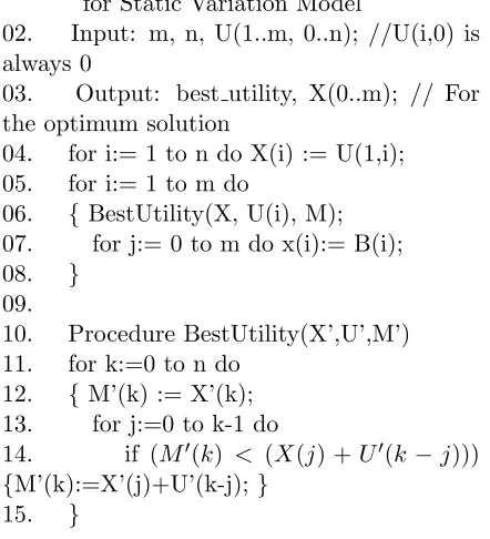
Actually, we can benefit even more. In such a situation, the “divide-and-conquer” algo-rithm in Figure 2 could be used. The divid-ing step iterates over the number of resources, while the merging step is performed in Proce-dure BestUtility. Since the utility for docu-ments in each resource is not related to any
01. Algorithm 2: Computing the Optimum Solution
for Static Variation Model
02. Input: m, n, U(1..m, 0..n); //U(i,0) is always 0
03. Output: best utility, X(0..m); // For the optimum solution
04. for i:= 1 to n do X(i) := U(1,i); 05. for i:= 1 to m do
06. { BestUtility(X, U(i), M); 07. for j:= 0 to m do x(i):= B(i); 08. }
09.
10. Procedure BestUtility(X’,U’,M’) 11. for k:=0 to n do
12. { M’(k) := X’(k); 13. for j:=0 to k-1 do
14. if (M′(k) < (X(j) +U′(k−j)))
[image:6.595.274.495.102.345.2]{M’(k):=X’(j)+U’(k-j);} 15. }
Figure 2: Algorithm for the Static Variation Model
other resource which contributes to the result, we can use the maximum computed for i re-sources in computing the maximum for i+ 1 resources. The time complexity of the algo-rithm isO(mn2).
4.2 Utility Function Analysis
Before further discussion, let us analyze the Utility function under Static Variation Model. For any giveni,U(i, j) only varies withj. We can rewrite Equation 6 as follow:
Udb(j) =k1Avg Rdb(j)−k2N Avg Tdb(j)−
−k3N Avg Cdb(j)−k4Avg Sdb (7)
Let us now discuss each of the four parts in Equation 7 one by one.
• Avg Sdb is invariant wrt j.
Doc(i) forms an arithmetic progression, that is, each document gets a certain amount less than its previous one when ordered by relevance. Then Avg Rdb(j)
(N Avg Rdb(j)) is a straight line with
negative slope.
• Connection time is one important part of all the time needed. It becomes a bigger part if only few documents are retrieved. If we assume that every document has the same size and the data transfer rate per unit time keeps constant, then
Avg Tdb(i, j) (N Avg Tdb(i, j)) is
mono-tonically decreasing with the number of documents j.
• As for charge, we simply consider the fol-lowing possible alternatives: a) a charge per unit of time; b) a charge per unit of data; c) a charge per document. Again, if we suppose every document has the same size and the data trans-fer rate per unit of time is constant, then the first two become identical. In such a situation, Avg Cdb(j) is just like Avg Tdb(j) in shape. In the third
situa-tion,Avg Cdb(j), just likeAvg Sdb, keeps
constant wrt variations of j. We can prove that in such situations the shape of
Pdb(j) can only be decreasing or
increas-ing monotonically, or firstly increasincreas-ing to a certain point then decreasing. What is more, the correspondingUdbvalues could
be different from one to another for differ-ent resources, still, their general shapes are always very similar to each other.
In practical situations, things could be more complicated especially for time and charge. We will not try to present any more detailed considerations fitting practical use.
4.3 A Greedy Algorithm and the Dynamic Variation Model
For reasons of space we will not be able to present here other two algorithms: the Greedy algorithm, which assumes that only one maximum exists in the utility function for each resource, and theDynamic Variation
Model, which remove the assumption related to the availability of similarities reported in the Static Variation Model. Both the Greedy algorithm and the Dynamic Variation Model bring the worst complexity of resource selec-tion to O(mn).
The details of these algorithm will be pre-sented in an extended version of this paper.
5 Conclusion
In this paper, we propose a multi-objective model for resource selection in distributed in-formation retrieval, in which four aspects are considered: document’s relevance to a given query, query time, query expense, and similar-ity between resources. An optimized solution is achieved by comparing the performances of all possible solutions. In addition, some vari-ations to the basic multi-objective model have been proposed as well, for more efficient im-plementations.
The following are some related issues demand-ing further consideration:
• In this paper we assume that relevance of documents to a query is normalized for all resources. However, that is not the usual case in practice. Further effort is needed, especially when each resource use a different indexing and retrieval model.
• A similarity measure between resources has been assumed throughout this paper, but how to define and implement such a measurement is not trivial.
• The algorithms presented in this paper (and some that could not be presented for space limitations) need further study with regards to their efficiency.
We are currently working in these directions.
Acknowledgements
References
[1] J. Callen, M. Connell, and A. Du. Au-tomatic discovery of language models for text databases. In Proceedings of ACM SIGMOD International Confer-ence, Philadelphia, USA, May 1999. [2] J.K. Callen, Z. Lu, and W. Croft.
Search-ing distributed collections with inference networks. InProceedings of the 18th an-nual International ACM SIGIR Confer-ence, Seattle, June 1995.
[3] N. Fuhr. A decision-theoretic approach to database selection in networked ir. ACM Transaction on Information Sys-tems, 17(3):229–249, 1999.
[4] H. Garcc´ıa-Molina and N. Shivakumar. A copy detection mechanism for digital documents. In Proceedings of 2nd Inter-national Conference in Theory and Prac-tice of Digital Libraries, Austin, USA, June 1995.
[5] L. Gravano and H. Garc´ıa-Molina. Gen-eralizing gloss to vector-space database and broker hierarchies. InProceedings of 21st VLDB Conference, Z˝urich, Switzer-land, 1995.
[6] D. Hawking and P. Thistlewaite. Meth-ods fro information server selection. ACM Transaction on Information Sys-tems, 17(1):40–76, January 1999.
[7] K. Monostori, A. Zaslavsky, and H. Schmit. Document overlap detection system for distributed digital libraries. In Proceedings of ACM International Conference on Digital Libraries, pages 226–227, San Antonio, June 2000.
[8] H. Nottelmann and N. Fuhr. MIND: an architecture for multimedia information retrieval in federated digital libraries. In Proceedings of the DELOS Workshop on Interoperability in Digital Libraries, Darmstadt, Germany, 2001.
[9] A. Powell, J. French, J. Callen, M. Con-nell, and C. Viles. The impact of
database selection on distributed search-ing. In Proceedings of ACM SIGIR Con-ference, pages 232–239, Athens, Greece, July 2000.