Scholarship@Western
Scholarship@Western
Electronic Thesis and Dissertation Repository
6-21-2017 12:00 AM
Efficient Macromodeling and Fast Transient Simulation of High
Efficient Macromodeling and Fast Transient Simulation of High
Speed Distributed Interconnects
Speed Distributed Interconnects
Sadia Wahid
The University of Western Ontario
Supervisor
Dr. Anestis Dounavis
The University of Western Ontario
Graduate Program in Electrical and Computer Engineering
A thesis submitted in partial fulfillment of the requirements for the degree in Master of Engineering Science
© Sadia Wahid 2017
Follow this and additional works at: https://ir.lib.uwo.ca/etd
Part of the Electrical and Electronics Commons, and the Systems and Communications Commons
Recommended Citation Recommended Citation
Wahid, Sadia, "Efficient Macromodeling and Fast Transient Simulation of High Speed Distributed Interconnects" (2017). Electronic Thesis and Dissertation Repository. 4649.
https://ir.lib.uwo.ca/etd/4649
This Dissertation/Thesis is brought to you for free and open access by Scholarship@Western. It has been accepted for inclusion in Electronic Thesis and Dissertation Repository by an authorized administrator of
In the first part of the thesis, an efficient macromodeling technique based on Loewner Matrix (LM) approach has been presented to model multi-port distributed systems using tabulated
noisy data. In the proposed method, Loewner Model data from previous rational approximation
are used to create less noisy eigenvectors in an iterative manner. As a result, the biasing effect of the LM model approximated by the noisy data is reduced. It is illustrated that this method
improves the accuracy of the Loewner Matrix modeling for noisy frequency data.
In the second part, a fast and robust algorithm is introduced for time-domain simulation of
interconnects with few nonlinear elements based on Large Change Sensitivity approach. After
macromodeling interconnects, linear parts of the system construct very large matrix. Large
linear matrix with nonlinear components makes time domain simulation a Central Processing
Unit (CPU) intensive task where inversion (one Lower/Upper (LU) decomposition and one for-ward/backward substitution) of this large matrix is done at each step of the Newton-Raphson iteration. Using the proposed method, large system matrix is partitioned into linear and
non-linear parts and LU decomposition of non-linear matrix is done only once in the entire simulation.
Nonlinear elements construct a very small matrix compared to large linear matrix. In this
pro-posed method, small matrix is inverted at each Newton iteration. Cost of inverting a small
matrix is much cheaper than inverting a very large matrix. Therefore, this approach is faster
than the conventional matrix inversion method. Numerical examples are presented illustrating
validity and efficiency of the above method.
Keywords: Frequency domain modeling, interconnect modeling, iterative Loewner method,
large change sensitivity, noisy frequency responses, transient analysis.
I would like to express my gratitude to my supervisor Dr. Anestis Dounavis for his guidance,
continuous encouragement, friendly motivation, patience, and his valuable advice during my
research journey. I am grateful to him for introducing me to the area of interconnect modeling
and simulations. Without his guidance and help this dissertation would not have been possible.
Moreover, I am thankful towards my colleagues: Tarik Menkad and Mohamed Sahouli for
sharing their knowledge and study materials, Sharath Manjunath for his help to set up my lab
desk and computer and Sara Mantach for her friendly conversations during my study period.
I would like to thank my family and friends for their motivation and persuasion throughout
my Master’s work. Finally, I must give greatest appreciation to my parents, for their love,
inspiration and support during my life so far.
To
my
Grandparents
Abstract i
Acknowledgment ii
Dedication iii
List of Figures vii
List of Tables x
List of Abbreviations xi
1 Introduction 1
1.1 Background and Motivation . . . 1
1.2 Objectives . . . 4
1.3 Contributions . . . 4
1.4 Organization of the Thesis . . . 4
2 High Speed Interconnects 6 2.1 Introduction . . . 6
2.2 Interconnect Modeling . . . 6
2.3 Quasi-Transverse Electromagnetic Models . . . 8
2.3.1 Distributed Lumped Modeling . . . 8
2.3.2 Method of Characteristics . . . 9
2.4 Full Wave Models . . . 12
2.5 Measured Data Model . . . 13
2.5.1 Vector Fitting . . . 13
2.6 Circuit Formulation of Distributed Networks . . . 18
2.6.1 Linear Distributed Networks . . . 19
2.6.2 Nonlinear Distributed Networks . . . 20
2.6.3 Nonlinear Network . . . 21
2.7 Transient Analysis of Nonlinear Network . . . 22
2.8 Conclusion . . . 23
3 Noisy Data Iterative Loewner Macromodeling 24 3.1 Introduction . . . 24
3.2 LM for Noisy Frequency Responses . . . 25
3.3 Proposed Algorithm . . . 28
3.3.1 Eigenvector Correction from Noise-free Data . . . 28
3.3.2 Eigenvector Correction from Noisy Data . . . 29
3.3.3 Description of Proposed Method with LM . . . 30
3.3.4 Methodology to Construct Previous Approximations with LM . . . 33
3.3.5 Order Selection . . . 34
3.4 Numerical Examples . . . 34
3.4.1 Example 1 . . . 35
3.4.2 Example 2 . . . 39
3.4.3 Example 3 . . . 45
3.4.4 Example 4 . . . 48
3.5 Limitations of Proposed Method . . . 49
3.6 Conclusion . . . 50
4 Fast Transient Analysis of Nonlinear Distributed Networks 53 4.1 Introduction . . . 53
4.2 Review of Large Change Sensitivity . . . 54
4.3 Large Change Sensitivity for Nonlinear Distributed Network Analysis . . . 56
4.3.1 Nonlinear Distributed Network Analysis . . . 56
4.3.2 Application of LCS for Nonlinear Distributed Network Analysis . . . . 57
4.4 Numerical Examples . . . 61
4.4.1 Example 1 . . . 61
4.4.2 Example 2 . . . 64
4.4.3 Example 3 . . . 66
4.4.4 Example 4 . . . 67
4.5 Limitations of Proposed LCS Method . . . 68
4.6 Conclusion . . . 69
5 Summary and Future Work 70 5.1 Summary . . . 70
5.2 Future Work . . . 71
Bibliography 73
Curriculum Vitae 80
2.1 Interconnect system top view and cross sectional view . . . 7
2.2 Distributed Lumped model segment . . . 9
2.3 Transmission Line Model for Method of Characteristics . . . 10
2.4 Linear Distributed Network . . . 19
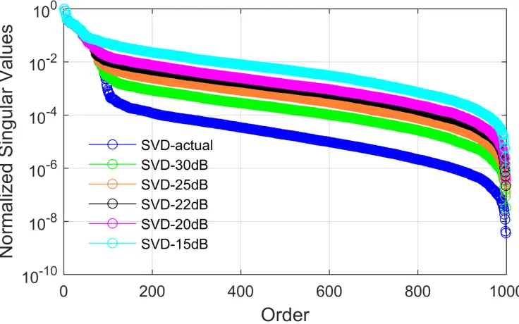
3.1 Normalized Singular Values (Example 2). . . 27
3.2 Normalized Singular Values (Example 3). . . 27
3.3 Rational Approximation of the 18-dB SNR data using Noisy Eigenvectors (blue) and Actual (Noise-free) Eigenvectors (red). (a) Real part and (b) Imaginary part plots (Example 1). . . 29
3.4 RMS error vs. order (Example 1) SNR=18dB . . . 33
3.5 Proposed RMS error vs. order (Example 1) SNR=18dB. . . 33
3.6 RMS error vs. order (Example 1) SNR=16dB. . . 33
3.7 Proposed RMS error vs. order (Example 1) SNR=16dB. . . 33
3.8 Rational Approximation of the 18-dB SNR data using LM and LM-Proposed approximation. (a) Real part and (b) Imaginary part plots (Example 1). . . 35
3.9 Normalized SVD versus Order (Example 1). . . 36
3.10 RMS error vs. iteration count for SNR=18 dB (Example 1). . . 36
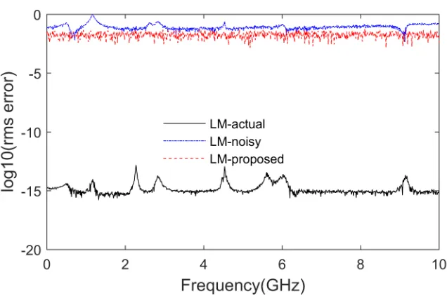
3.11 Log10(RMS error) vs. frequency plots for actual (noise-free) data approxima-tion with LM (black), noisy data approximaapproxima-tion with LM (blue) and noisy data approximation with LM-proposed (red) (Example 1) . . . 37
3.12 Rational Approximation of the 16-dB SNR data using LM and LM-Proposed approximation. (a) Real part and (b) Imaginary part plots (Example 1). . . 37
3.13 Transmission line network (Example 2) . . . 39
3.15 Normalized Singular Values (Example 2) . . . 40
3.16 Rational Approximation of Y(1,3) (Example 2)(SNR=25dB). . . 40
3.17 Rational Approximation of Y(2,3) (Example 2) (SNR=25dB). . . 41
3.18 Rational Approximation of Y(2,2) (Example 2) (SNR=25dB). . . 41
3.19 RMS error versus iteration count for SNR=25 dB (Example 2). . . 42
3.20 H2-norm error versus iteration count for SNR=25 dB (Example 2) . . . 42
3.21 LM approximation of actual/noise-free data (black), LM approximation with noisy data (Blue) and proposed method approximation (Red) for order 105 (Example 2) (SNR=25dB) . . . 42
3.22 Rational Approximation of Y(1,3) (Example 2) (SNR=20dB) . . . 43
3.23 Rational Approximation of Y(2, 3) (Example 2) (SNR=20dB). . . 43
3.24 Rational Approximation of Y(2, 2) (Example 2) (SNR=20dB). . . 44
3.25 RMS error versus iteration count for SNR=20 dB (Example 2). . . 44
3.26 H2-norm error versus iteration count for SNR=20 dB (Example 2) . . . 44
3.27 LM approximation of actual (noise-free) data (Black), LM approximation with noisy data (Blue) and proposed method approximation (Red) for order 120 (Example 2) (SNR=20dB) . . . 45
3.28 Circuit Diagram (Example 3) . . . 46
3.29 Normalized singular values vs. order for SNR=30dB (Example 3) . . . 47
3.30 log10(H2error) vs. order for SNR=30 dB (Example 3) . . . 47
3.31 ProposedH2 error vs. order for SNR=30 dB (Example 3) . . . 47
3.32 Rational Approximation of Y(1,18) (Example 3). . . 47
3.33 Rational Approximation of Y(17,18) (Example 3). . . 48
3.34 Rational Approximation of Y(6,10) (Example 3). . . 48
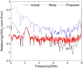
3.35 Relative Error of actual (noise-free) data LM approximation, noisy data LM approximation and proposed method LM approximation (Example 3) . . . 49
3.36 Four-port network (Example 4). . . 49
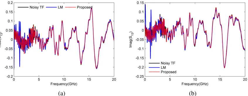
3.37 Rational Approximation of S(1,3) (Example 4). . . 50
3.38 Rational Approximation of S(2, 3) (Example 4). . . 50
3.41 H2-norm error versus iteration count (Example 4) . . . 51
3.42 Relative Error of LM and Proposed Method (Example 4) . . . 51
4.1 Illustrative LCS example . . . 59
4.2 Circuit containing three lossy TLs (Example 1) . . . 62
4.3 Transient response of the circuit shown in Figure 4.1 at nodeVout . . . 64
4.4 Error at nodeVout . . . 64
4.5 Circuit of (Example 2) . . . 65
4.6 Transient Analysis at node M1 of Example 2 . . . 66
4.7 Circuit of (Example 3) . . . 66
4.8 Transient Analysis at node P1 of Example 3 . . . 67
4.9 Circuit of (Example 4) . . . 67
4.10 Transient Analysis at port 10 (Example 4) . . . 68
3.1 Poles and Residues of the TF (Example 1) . . . 35
3.2 Calculated Poles Using LM and proposed method (Example 1) (SNR=18 dB) . 38 3.3 Calculated Poles Using LM and proposed method (Example 1) (SNR=16 dB) . 38 3.4 100 simulations with different random noise (Example 1) . . . 38 4.1 Simulation Results using Conventinal matrix inversion and Proposed LCS method 63
VLSI Very Large Scale Integration.
LM Loewner Matrix.
MNA Modified Nodal Analysis.
DS Descriptor System.
LU Lower-Upper matrix decomposition.
ODE Ordinary Differential Equations.
LCS Large Change Sensitivity.
PDE Partial Differential Equations.
SNR Signal-to-Noise Ratio.
VF Vector Fitting.
MoC Method of Characteristics.
PRIMA Passive Reduced-order Interconnect Macromodeling Algorithm.
SVD Singular Value Decomposition.
VNA Vector Network Analyzer.
Introduction
1.1
Background and Motivation
Advances in Very-Large-Scale-Integration (VLSI) technology have made phenomenal growth
in operating speed, densities and diminishing device sizes. With increasing frequency,
inter-connect analysis has become a major requirement for all state-of-the-art circuit design and
sim-ulations. Interconnects can exist at various levels such as on-chip, packaging structures, vias,
printed circuit boards (PCB) and backplanes etc. Once neglected interconnect effects such as ringing, signal delay, distortion and attenuation give rise to signal integrity issues [1–5].
Accu-rate capture of signal integrity issues at early stage of design ensures circuit performance and
reliability [1].
Circuit simulators like SPICE face difficulties to simulate interconnects in the presence of nonlinear components due to mixed frequency/time problem as well as CPU inefficiency. This is because, characteristics of interconnects are governed by Telegrapher’s equations which are
Partial Differential Equations (PDEs) and are best solved in the frequency domain, whereas nonlinear elements are described only in the time domain with nonlinear Ordinary Differential Equations (ODEs). Different numerical macromodeling techniques are used to convert PDEs to ODEs to simulate interconnects with nonlinear elements [1, 3, 5, 6].
At first we can divide interconnect macromodeling strategies into two cases. In the first case,
physical characteristics of the interconnect structure are known and modeling is based on
Quasi-Transverse Electromagnetic mode of propagation of waves. In the second case, where
physical structure is unknown or any analytic solution is hard to derive, rational
macromodel-ing approximation from full-wave electromagnetic simulation or port-port measured data are
used to model interconnects [7].
Two types of macromodeling are done with known physical characteristics of interconnects.
One is rational approximation and other is delay extraction based modeling techniques. Brute
force lumped segmentation modeling [8], passive reduced-order interconnect
macromodel-ing algorithm (PRIMA) [9], matrix rational approximation (MRA) [10, 11], compact diff er-ence [12], integral congruent transformation [13, 14] are included under rational
approxima-tion modeling. These modeling algorithms are passive by construcapproxima-tion. However, they require
high order approximation to capture the delay. On the other hand, delay extraction method
like Method of Characteristics (MoC) [15] use a low order approximation as the delay of the
transfer function is extracted. However, MoC is not passive by construction.
Macromodeling algorithms for interconnects with no prior knowledge of the physical
charac-teristics are based on frequency domain, multiport tabulated data obtained either from
elec-tromagnetic simulations or from measurements [16–37]. Frequency domain data are often
presented in the form of impedance, hybrid, scattering or admittance parameters data. One
approach to convert frequency domain data into time domain analysis is based on convolution
techniques [19, 20]. However, this approach is time consuming [21] and requires high
mem-ory allocation [22]. Another approach is to generate closed form time domain macromodels.
These methods approximate the transfer function in descriptor system (DS) or pole-residue
for-mat. They can be directly incorporated into modified nodal analysis equations [23] or recursive
convolution can be used to obtain transient response [24].
A popular pole-residue based system identification tool is called Vector Fitting (VF) [16] which
approach to improve the approximation. Various enhancements have been made to improve
its accuracy and efficiency [25–27]. VF has also been used for multiport network using QR decomposition and parallel processing [28]. In recent years, Loewner Matrix (LM) [29–31]
framework has been proposed to generate descriptor state-space models from frequency
do-main measured data of interconnect network. Unlike VF, LM method is very efficient to iden-tify the system from the tabulated data with fewer state-space equations [29, 31]. In Loewner
Matrix modeling, order of the system can be identified from the Singular Value Decomposition
(SVD) of Loewner Matrix [29]. Delay extraction based Loewner modeling method has been
proposed in [32] to approximate a low-order rational model.
In the presence of noise in frequency domain data, several modifications have been proposed
for vector fitting algorithm. They are such as pole adding and skimming method [33], least
squares weighted functions [34] and instrumental variable VF method [35]. Moreover, LM
interpolation method faces some issues to accurately identify the system from contaminated
frequency domain data [36]. In [36] which pole/residues are relevant based on examining the norms of the residues and in [37] an iterative least square based LM interpolation
approxima-tion are proposed to identify system from noisy data, respectively.
After macromodeling interconnects, nonlinear components like drivers and receivers are
in-cluded in time domain circuit simulations. For transient analysis, integration techniques are
used to convert differential equations into difference equations. To solve the difference equa-tions with nonlinear elements at each time step, Newton-Raphson iteraequa-tions are required.
Mod-eling of interconnects leads to large circuit matrix making time-domain analysis a CPU
inten-sive task for nonlinear circuit simulators [3]. In order to address the above issue, a fast and
1.2
Objectives
The first objective of this thesis is to develop an algorithm to improve the accuracy of the
identified state-space system from the noisy data based on Loewner modeling approach. The
second objective is to apply Large Change Sensitivity (LCS) [38,39] approach for fast transient
analysis of interconnects circuits including nonlinear loads, drivers and receivers.
1.3
Contributions
The main contributions of the thesis are as follows:
1. An iterative algorithm is proposed to create less noisy data from previous Loewner
Matrix approximated model. Then this data is used to create less noisy eigenvectors. As a
result, the biasing effect of the LM solution caused by the noise of the eigenvectors created from original data is reduced by this method.
2. This proposed iterative method has been applied to multiport network. Numerical
ex-amples are presented to compare the LM based approximation and proposed iterative LM
ap-proximated models.
3. Large Change Sensitivity approach is used for fast transient analysis of large distributed
networks terminated with nonlinear loads and drivers.
4. LM method has been used to model large interconnect network from measured frequency
data. Loewner method together with Large Change Sensitivity (LCS) approach is used for
transient analysis of nonlinear distributed networks.
1.4
Organization of the Thesis
The organization of the thesis is as follows. Chapter 2 gives brief review of interconnects
modeling, modified nodal analysis of linear and nonlinear distributed networks and transient
multiport systems characterized by noisy frequency domain data, using an iterative Loewner
Matrix algorithm. It is illustrated that the proposed approach can increase the accuracy of
the Loewner modeling with noisy tabulated data. Chapter 4 discusses a fast transient analysis
algorithm based on Large Change Sensitivity approach. Here distributed interconnect network
has been modeled using lumped modeling and Loewner matrix modeling techniques. Time and
accuracy have been compared between conventional matrix inversion and proposed approach
for transient analysis for both modeling approaches. Finally, Chapter 5 summarises the work
High Speed Interconnects
2.1
Introduction
Interconnects propagate signals between electrical devices. At low frequencies, they behave
like short circuits. As the frequency increases, they start to behave like transmission lines
and are responsible for signal degradation in the circuit. Modern VLSI circuits have made
modeling and analyzing of interconnects a necessary task. The aim of this chapter is to review
some of the interconnect macromodels and numerical techniques that are used for interconnect
analysis.
2.2
Interconnect Modeling
Interconnect modeling depends on the physical structure as well as the operating frequency
of the electrical circuit. Electrical lengthof interconnects is an essential factor to model and analyze them. Interconnects are considered to be ‘electrically short’, if they are physically shorter than one-tenth of the wavelength of the operating signal [3].
l
λ <0.1; λ=
v
f (2.1)
where l is the interconnect length, λ is the signal wavelength, v is the propagation velocity and f is the frequency. Otherwise, interconnects are considered,‘electrically long’. A practical relationship between maximum frequency denoted by fmaxand rise time represented astrof a
signal can be expressed as [3, 40],
fmax≈
0.35
tr
(2.2)
Figure 2.1 shows the top view and cross sectional view of an interconnect system consists of
Figure 2.1: Interconnect system top view and cross sectional view
four conductors and ground plane. Modeling of interconnects depends on the operating
fre-quency, signal rise and fall times, length of interconnects and their physical properties. These
factors determine whether the modeling of interconnects is based on quasi-transverse
electro-magnetic (quasi-TEM) or full wave assumptions. For interconnect structure that cannot be
modeled analytically, linear networks characterized by tabulated or measured data have been
2.3
Quasi-Transverse Electromagnetic Models
Transverse electromagnetic (TEM) waves exist for interconnects with homogeneous mediums
and perfect conductors [2]. Under these conditions, interconnects produce electric and
mag-netic fields that are transverse or perpendicular to one another and to the direction of
propa-gation. Quasi-TEM assumptions remain the dominant trend for analyzing interconnects, since
the approximation is valid for most practical structures and offers relative ease and low com-putation cost compared to full wave approaches [3, 5].
The voltages and currents for interconnects under quasi-TEM assumption are described by
partial differential equations (PDEs) known as Telegrapher’s equations,
∂v(x,t)
∂x = −Ri(x,t)−L
∂i(x,t)
∂t
∂i(x,t)
∂x =−Gv(x,t)−C
∂v(x,t)
∂t (2.3)
where voltagev(x,t) and currenti(x,t) are functions of positionxand timet;R, L,CandGare the per unit length (p.u.l.) resistance, inductance, capacitance and conductance of the
intercon-nect respectively. The p.u.l parameters are obtained from the cross-sectional dimensions and
physical characteristics of the transmission line. They are also used to determine voltages and
currents of the transmission line [2].
2.3.1
Distributed Lumped Modeling
Lumped segmentation technique uses lumped resistive-inductive-conductive-capacitive (RLGC)
model of the transmission lines to approximate Telegrapher’s equations. Applying Euler’s
method [2] to (2.3) yields
v(x+ ∆x,t)−v(x,t)= −∆xRi(x,t)−∆xL∂i(x,t)
∂t
i(x+ ∆x,t)−i(x,t)=−∆xGv(x+ ∆x,t)−∆xC∂v(x+ ∆x,t)
where x = [1,2, ..., η], ∆x = l/η, ηis the number of sections andl is the length of intercon-nect. Equation (2.4) can be implemented by lumped equivalent circuit composed of resistors,
inductors, conductors, and capacitors.
Figure 2.2: Distributed Lumped model segment
Figure 2.2 shows the general lumped component for a two conductor transmission line. HSPICE
[41] use equation (2.5) in order to estimate the number of sections for time domain analysis of
interconnects.
η=20l.
√
LC tr
(2.5)
wheretris the rise/fall time. The lumped segmentation model is passive and provides a direct
method to discretize interconnects. However the approximation is only valid if ∆x is chosen to be a small fraction of the wave length. If the rise/fall time is fast or if the interconnect is electrically long, many lumped segments are required for an accurate model. This leads to
large circuit matrix increasing CPU time for time domain simulation.
2.3.2
Method of Characteristics
Another most commonly used algorithms to model interconnect are based on the generalized
ex-tracted and exact models are produced applying to lossless transmission lines [15]. These
methods are also applied to model lossy MTLs [42–46]. The MoC is based on extracting
the propagation delay allowing the attenuation function to be approximated with a low order
rational transfer function. It reduces the computation complexity for long lines with low losses.
The original method of characteristics [15] or Branin’s method was used to represent
inter-connects as ODEs containing time delays. Although it was developed in the time-domain
using characteristics curves (hence the name), a simpler alternative in the frequency domain is
presented here. The frequency domain solution of Telegrapher’s equation for two-conductor
transmission lines (one signal conductor and another reference conductor) [46] is
I1 I2 = 1
Z0(1−e−2γl)
1+e−2γl −2e−γl
−2e−γl 1+e−2γl V1 V2 (2.6)
γ = p
(R+sL)(G+sC) Z0=
r
R+ sL G+ sC
whereγis the propagation constant andZ0is the characteristics impedance.
Figure 2.3: Transmission Line Model for Method of Characteristics
After some re-arrangement, the terms in (2.6) can be expressed as,
V1= Z0I1+W1
HereW1andW2have a recursive relation as
W1 =e−γl(2V2−W2)
W2 =e−γl(2V1−W1) (2.8)
For lossless transmission lines,R= 0 andG= 0. ThusγandZ0reduces to
γ = s
√
LC Z0 =
r
L
C (2.9)
As a result,γbecomes purely imaginary andZ0becomes a real constant. By taking the inverse
Laplace transform of (2.7) & (2.8), we can get the time domain solution of MoC as,
v1(t)= Z0i1(t)+w1(t) v2(t)= Z0i2(t)+w2(t) w1(t+τ)=2v2(t)−w2(t)
w2(t+τ)=2v1(t)−w1(t) (2.10)
whereτ= γlis a delay term in the domain. A transmission line model for MoC in time-domain is shown in Figure 2.3. For lossy transmission lines,γ is not purely imaginary andZ0
is not a real constant. They are irrational function of complex frequencys. As a result, direct time domain representation is not possible. In this case, rational approximation ofγandZ0has
Therefore,γandZ0are approximated as,
Z0 = Z0(s)'
X
n
RZ n
s−pZ n
+Z∞
γ= γ(s)= p(R+sL)(G+sC)≈ spL∞C∞+P(s) P(s)' X
n
RPn
s− pP n
+P∞
Here Z0(s) and P(s) are approximated in pole residue form. RZn and p Z
n are real or complex
residues and poles ofZ0(s). RPn and p P
n are real or complex residues and poles ofP(s). L∞,C∞
are inductance and capacitance ats= j∞respectively.
2.4
Full Wave Models
If the cross-sectional dimensions of interconnects become a significant fraction of the circuits
operating wavelength, field components in the direction of propagation can no longer be
ig-nored [47]. Under these conditions, quasi-TEM assumptions become inadequate to describe
interconnect and full wave models are required.
Full wave models provide better accuracy when compared to quasi-TEM models. However,
full wave models are not used by circuit simulators because of the expensive CPU
require-ments [48]. The cost of full wave simulation associated with each interconnect at a particular
frequency point is extremely high. Generally, high speed interconnects require thousands of
frequency points to accurately model the response of the system. The cost of the
computa-tion of the full wave model combined with the evaluacomputa-tion cost of the overall circuit makes the
technique unreasonably expensive to use in circuit simulation.
Another problem with full wave methods is to represent the model in the circuit simulator.
The information provided by wave full wave analysis is in terms of field parameters such as
propagation constants, characteristic impedances, current eigenvectors, etc. Circuit simulators
needs to be developed to link full wave methods into circuit simulators.
2.5
Measured Data Model
For interconnects having geometric inhomogeneity and discontinuities, sometimes it is not
possible to obtain accurate analytical physics based models. To overcome this issue, modeling
techniques based on measured data or tabulated data have been proposed [49,50]. Interconnects
are modeled using measured data from frequency dependent scattering parameters,
electromag-netic simulations or by time domain terminal measurements. Time domain measurements can
be acquired by numerical solution of the electromagnetic field problems [51, 52] or by time
domain reflectometry (TDR) methods [53]. Measured data obtained by different methods are contaminated by noise. To decrease the impact of noise, large data sets are required.
2.5.1
Vector Fitting
Vector fitting (VF) uses an iterative approach to acquire a rational function to approximate
the data obtained by measurement or electromagnetic simulation. It was first introduced by
Gustavsen in 1998 and many developments have been made over the years in [16, 54–57].
The objective of vector fitting is to determine a rational approximation of a set of measured
data{s,Y(s)}as,
f(s)=
N X
n=1 rn
s− pn
+d+ se (2.11)
where rn and pn correspond to real or conjugate residues and poles respectively, while the
real variables d and e are optional; sis the Laplace variable,Y(s) is the measured data value at s and N is the number of poles and residues or the order of the rational function. The nonlinear problem in (2.11) can be solved by following two steps. The first step is an iterative
pole identification process and the second step is to identify the residues using a least square
introduced as,
α(s)=
N X
n=1
˜
rn
s− p˜n
+1 (2.12)
where ˜pnare the starting poles and the remaining terms are unknowns. In addition, the rational
approximation forα(s)f(s) can be described as,
α(s)f(s)(αf)(s)= N X
n=1 rn
s−p˜n
+d+se (2.13)
Multiplying (2.12) by f(s) and equating with (2.13), yields the following system of equation,
N X
n=1 rn
s− p˜n
+d+ se=(
N X
n=1
˜
rn
s− p˜n
+1)f(s) (2.14)
This linear problem hasrn, ˜rn, d andeas unknowns. For each frequency pointsj, the system
of (2.14) can be expressed as,
AjX =bj (2.15)
where
Aj =
Re(z1j) .... Re(zNj) 1 0 Re(˜z1j) .... Re(˜zNj)
Im(z1j) .... Im(zNj) 1 0 Im(˜z1j) .... Im(˜zNj)
X =
r1 .... rN d e r˜1 .... r˜N
(2.16)
bj =
Re(Y(sj))
Im(Y(sj))
For real poles and residues, the coefficients of (2.16) will become,
zkj = 1 sj −p˜k
; z˜kj = −Y(sj)
For complex conjugate pole and residue pairs, the coefficients of (2.16) will be
zkj = 1 sj− p˜k
+ 1
sj− p˜k+1
; zkj+1= i sj− p˜k
− i
sj− p˜k+1
˜
zkj = −Y(sj) sj− p˜k
+ −Y(sj)
sj −p˜k+1
; z˜kj+1 = −iY(sj)
sj− p˜k
+ iY(sj)
sj− p˜k+1 rk = Re(rk); rk+1= Re(rk)
˜
rk = Re(˜rk); r˜k+1= Re(˜rk)
From all the above equations, an overdetermined system of equation can be formed for all the
frequency points as,
AX = b (2.17)
The solution ofXcan be obtained by the least square solution by doing,
X= (ATA)−1(ATb) (2.18)
From the least square solution of (2.18), we can get approximations forα(s) and (αf)(s) and they can be written as,
α(s)f it = QN
n=1(s−a˜n) QN
n=1(s− p˜n)
(αf)f it(s)=e QN+1
n=1(s−an) QN
n=1(s− p˜n)
(2.19)
The poles of (2.19) cancel each other out to get a rational approximation for f(s) as,
f(s)= (αf)f it(s)
α(s)f it
=e
QN+1
n=1(s−an) QN
n=1(s−a˜n)
(2.20)
where the zeros of α(s)f it becomes the poles of f(s). By taking this new set of poles ˜an as
the new guess for the next iterations to replace previous poles pn. This iterative procedure is
After the poles of the system are determined, an additional least square solution is needed for
the residues to obtain and the termsdandeif they are present in the system.
2.5.2
Loewner Matrix Model
In time domain, a multiport Linear Time Invariant (LTI) system withPinputs and outputs can be described as a state-space model:
Ex˙(t)= Ax(t)+ Bu(t)
y(t)=Cx(t)+ Du(t) (2.21)
where x(t) ∈ Rr vector contains internal variables,u(t) ∈ RP andy(t) ∈ RP vectors contains
input and output port voltages and currents, respectively. The matricesE,A∈Rr×r,B∈Rr×P,
C ∈ RP×r, D ∈ Rr×P describe the system and r is the order of the system. The closed form
expression of frequency domain Y-parameters of the LTI system in (2.21) can be presented by,
Y(s)=C(sE− A)−1B+ D (2.22)
Loewner Matrix method [29–31] is used to get a time domain macromodel from the frequency
domain measured or simulated data. Frequency domain data are often presented in the form of
impedance, hybrid, scattering (S-parameter) or admittance (Y-parameter) parameter data.
The frequency domain data is expressed as,
{sm,Y(sm)} (2.23)
wheresmis the complex frequency,Y(sm) is theS-parameter orY-parameter data at frequency
into odd and even data points as follows:
{s1, . . . ,sM}= {τ1, . . . , τm} ∪ {υ1, . . . , υm}
{Y(s1), . . . ,Y(sM)}={Y(τ1), . . . ,Y(τm)} ∪ {Y(υ1), . . . ,Y(υm)}
{Y(τ1), . . . ,Y(τm)}= {W1, . . . ,Wm}
{Y(υ1), . . . ,Y(υm)}={U1, . . . ,Um}
(2.24)
Herem+m= M.
m=m= M
2 Here M is even
m= m+1= M+1
2 Here M is odd
Here frequency data is splitted into odd and even data points.
Right data set:
Γ=diag[τ1, . . . , τm]∈Cm×m, R=[R1, . . . ,Rm]∈CP×m,W= [W1, . . . ,Wm]∈CP×m
Left data set:
Υ= diag[υ1, . . . , υm] ∈ Cm×m, LT = [L1, . . . ,Lm] ∈ Cm×P, UT = [U1, . . . ,Um] ∈ Cm×P
Here Rand L are random matrices. Loewner matrix Land shifted Loewner Matrix σLare
calculated as: L=
U1R1−L1W1
υ1−τ1 . . .
U1Rm−L1Wm
υ1−τm
... ... ... UmR1−LmW1
υm−τ1 . . .
UmRm−LmWm
υm−τm
(2.25)
σL=
υ1U1R1−τ1L1W1
υ1−τ1 . . .
υ1U1Rm−τmL1Wm
υ1−τm
... ... ...
υmUmR1−τ1LmW1
υm−τ1 . . .
υmUmRm−τmLmWm
υm−τm
(2.26)
The LMs are complex matrices. In order to get a real macromodel, a similarity transformaion
is used as follows [29, 31]
LR = T
∗LT, σL R =T
UR =T ∗
U, WR = TW (2.27)
where,
T= blkdiag[t, . . . ,t]∈Cm×m, t= √1
2
1 −j
1 +j
According to [29] state-space realization of the time domain model can be extracted from the
regular part of the Loewner Matrix pencil (sLR−σLR). The regular part is extracted from SVD
of (sLR − σLR). Any value of s can be chosen unless it is not the eigenvalue of (LR, σLR).
Using singular value decomposition (SVD), the realization can be obtained as follows:
S V D(sLR−σLR)= YΣX;
rank(sLR−σLR)= rank(Σ)= r;
Y1 ∈Rm×r and X1∈Rm×r
(2.28)
Here order or rank of the system isr. HereYandXare left and right eigenvectors. Y1andX1
are constructed from the firstrcolumns ofYandX. The system matrices are defined as,
E= Y∗1LRX1; A=Y1∗σLRX1;
B= Y∗1UR; C=−WRX1; D= 0;
(2.29)
At this stage Dmatrix is always zero. Sometimes embedded Dmatrix is needed to be extracted
to get a stable macromodel as illustrated in [31].
2.6
Circuit Formulation of Distributed Networks
Figure 2.4: Linear Distributed Network
2.6.1
Linear Distributed Networks
Let us consider the linear distributed network shown in Figure 2.4. The Modified Nodal
Anal-ysis (MNA) equation can be expressed in time domain as,
G1 0
0 0 v1 v2 + 0 0
0 C2
dv1 dt dv2 dt + i1 i2 =
J(t) 0 (2.30)
In the frequency domain, Y-parameter expression of the 2-port distributed network in Figure
2.4 can be expressed as,
I1 I2 =
Y11 Y12
Y21 Y22
V1 V2 (2.31)
After macromodeling the distributed network using Loewner modeling, let us considerr ele-ments are present in the port system. In the time domain, following equation (2.21) state space
equation for this 2-port system can be written as,
e11 . . . e1r ... ... ...
er1 . . . err dx1 dt ... dxr dt =
a11 . . . a1r ... ... ...
ar1 . . . arr x1 ... xr +
b11 b12
... ...
br1 br2
i1 i2 =
c11 . . . c1r
c21 . . . c2r x1 ... xr +
d11 d12 d21 d22
v1 v2 (2.33)
Now equations (2.32) and (2.33) are embedded in equation (2.30). We first substitute (2.33)
intoi1 andi2in (2.30). We obtain an equation with parameterx= [x1. . .xr] as,
G1+d11 d12 c11 . . . c1r
d21 d22 c21 . . . c2r v1 v2 x1 ... xr +
0 0 0 . . . 0
0 C2 0 . . . 0
dv1 dt dv2 dt dx1 dt ... dxr dt =
J(t) 0 0 ... 0 (2.34)
Now we add equation (2.32) to the bottom of equation (2.34). We can get the integrated MNA
equation for the whole circuit shown in Figure 2.4 as,
G1+d11 d12 c11 . . . c1r
d21 d22 c21 . . . c2r
−b11 −b12 −a11 . . . −a1r ... ... ... ... ...
−br1 −br2 −ar1 . . . −arr v1 v2 x1 ... xr +
0 0 0 . . . 0
0 C2 0 . . . 0
0 0 e11 . . . e1r ... ... ... ... ...
0 0 er1 . . . err dv1 dt dv2 dt dx1 dt ... dxr dt =
J(t) 0 0 ... 0 (2.35)
2.6.2
Nonlinear Distributed Networks
In general, distributed networks in the presence of nonlinear elements can be expressed as [5]
Cφdxφ(t)
dt +Gφxφ(t)+
Nt
X
k=1
Ik(s)=Vk(s)Yk(s) (2.36)
where
• xφ(t) is a vector, which includes node voltages appended by independent and dependent voltage source currents, inductor currents, nonlinear capacitor charge, and nonlinear
in-ductor flux waveform. Gφ andCφ are constant matrices describing the lumped memo-ryless and memory elements of the network, respectively. bφ(t) is a vector with entries
determined by the independent voltage and current sources. F(xφ(t)) is a vector
describ-ing the nonlinear elements.
• Dk = [di,j ∈ {0,1}] is a selector matrix that maps the vector of terminal currents ik(t)
entering the interconnectkinto the node space of the circuit network, wherei∈1, . . . , φ,
j ∈ 1, . . . ,2Mk and Mk is the number of coupled signal conductors in the kth
intercon-nect. Nt is the number of distributed structures. Yk(s) is the admittance parameters of
interconnect subnetwork in the Laplace domain. Vk(s) and Ik(s) represent the Laplace
terminal voltages and currents of interconnectk.
2.6.3
Nonlinear Network
After macromodeling the distributed transmission lines into ODEs, large nonlinear
intercon-nect network can be expressed by,
Cψdx(t)
dt +Gψ(t)+F(x(t))= b(t) (2.37)
2.7
Transient Analysis of Nonlinear Network
The time domain solution of (2.37) is derived by converting the nonlinear differential equa-tions to nonlinear algebraic equaequa-tions using explicit method such as Forward Euler and implicit
methods like Backward Euler and Trapezoidal rule. Explicit methods require no matrix
inver-sion making them computationally less expensive than implicit methods that require matrix
inversion. But explicit methods are never used for circuit simulation as they are not absolutely
stable for all step sizes. On the other hand, implicit methods are absolutely stable and used
for solving nonlinear circuits with Newton-Raphson iteration at each time step. For multinode
network after using Trapezoidal rule difference equation of (2.37) can be written as
(Cψ
∆t + Gψ
2 )xt+1+
F(xt+1)
2 −(
Cψ ∆t −
Gψ
2 )xt+
F(xt)
2 =
bt+bt+1
2 (2.38)
Here∆tis the step size. Let us consider step size∆tis very small and does not change during time domain simulation.
After applying Newton-Raphson method the problem becomes solving the following function,
ftk+1 = ( Cψ
∆t + Gψ
2 )xt+1 +
F(xt+1)
2 − (
Cψ ∆t −
Gψ
2 )xt +
F(xt)
2 −
bt+bt+1
2 = 0 (2.39)
where xt+1is the unknown vector with n number of variables to be solved at each iteration by
applying,
xkt++11 = xtk+1+ ∆xkt+1 (2.40)
∆xkt+1= −(Mtk+1)−1ftk+1 (2.41)
wherekis the iteration number. HereMis ann×nJacobian matrix and can be expressed as,
Mk t+1 =(
Cψ ∆t +
Gψ
2 )+ 1 2
dF(xk t+1) dxt+1
(2.42)
the Jacobian matrix in equation (2.42). Each iteration costs one LU factorization and one
forward/backward substitution.
In the Jacobian matrix,Cψ andGψ are very large matrices. To invert the Jacobian matrix at each step of Newton iteration becomes a CPU intensive task for time domain analysis. This
issue has been addressed in this thesis.
2.8
Conclusion
In this chapter, an overview of different macromodeling techniques of interconnect is given based on known and unknown physical characteristics of the structures. Furthermore, MNA
equations are derived for Loewner matrix modeling technique. Finally, a brief review of
Noisy Data Iterative Loewner
Macromodeling
3.1
Introduction
System identification has become a challenging task for high speed devices and structures. To
identify a system without any prior knowledge of physical characteristics is based on frequency
domain tabulated data. Recently Loewner Matrix (LM) [29–31] based method was proposed to
generate state-space macromodels from frequency domain measured data. This method faces
difficulty to identify a system accurately from contaminated noisy frequency data [36]. This chapter presents an iterative method to macromodel a system from frequency data
contami-nated by noise based on Loewner Matrix framework. In this proposed algorithm, eigenvectors
are generated from previous Loewner Matrix approximated model. As previous approximated
model has less noise in it than the original data, it is illustrated that this method will give
better approximation of Loewner matrix method thus improving the accuracy of the
approxi-mated Loewner matrix model. Numerical examples are provided to demonstrate the validity
and accuracy of the proposed method.
3.2
LM for Noisy Frequency Responses
A single port or a multiport network can be characterized by measured data in the form of
admittance, impedance, hybrid or scattering parameter data. Let us consider that the frequency
domain scattering (S-parameter) or admittance (Y-parameter) data can be expressed as,
{sm,Y(sm)}
Y(sm)=[Yi j(sm)] (i, j∈1, ....,P)
(3.1)
where,smis the complex frequency,Y(sm) is theS-parameter orY-parameter data at frequency
sm,m =1,2, . . . ,M, whereMis the number of data points andPis the number of ports of the
network. Let us consider the frequency domain noisy data as,
˜
Y(sm)= Y(sm)+(sm) (3.2)
Here ˜Y is the contaminated data and is a zero-mean random noise (meaning the expected
mean valueE[] is zero).
From noisy data set{sm,Y˜(sm)}, using equation (2.24) right and left noisy complex data
matri-ces ˜Wand ˜Uare created respectively and can be expressed as,
˜
W=W+HW
˜
U= U+HU
(3.3)
HereHW andHU are due to noisein the data. Asis a zero mean randon noise, the expected
mean values ofHW andHU are zero.
E[HW]=0
E[HU]=0
(3.4)
matrices are created and can be expressed as,
˜
WR =WR+HWR
˜
UR =UR+HUR
˜
LR =LR+HUR +HWR
˜
σLR =σLR+HUR +HWR
(3.5)
Here ˜WR, ˜UR, ˜LR,σL˜R are real right data noisy matrix, real left data noisy matrix, real noisy
Loewner matrix and real noisy shifted Loewner matrix from given noisy data respectively.
HWR and HUR comes from the noisy data matrices ˜W and ˜U, respectively. Since expected
mean valueE[] is zero, expected mean values ofHWR andHUR are also zero.
E[HWR]= 0
E[HUR]=0
(3.6)
HWR and HUR matrices do not statistically bias the results of LM approximation. However,
Singular Value Decomposition (SVD) of Loewner Matrix and shifted Loewner Matrix is
per-tubed as bellow,
S V D(sL˜R−σL˜R)= Y˜Σ˜X˜; (3.7)
For different example perturbation of SVD of Loewner matrices is different. SVD of noisy Loewner Matrices of Example 2 & 3 (which are described later in Chapter 3) are given in
Figure 3.1 & 3.2, respectively. In these figures different noise values are added to frequency domain data to see the change of SVD of Loewner matrices. As a result, from equation (3.7)
left and right eigenvectors ˜Yand ˜X, respectively, has noise in it.
˜
Y and ˜X are noisy left and right eigenvectors. Y˜1 and ˜X1 are constructed from the first r
columns of ˜Yand ˜X.
˜
Y1 =Y1+Y1UR +Y1WR
˜
X1 =X1+X1UR +XW1 R
Figure 3.1: Normalized Singular Values (Example 2).
HereYUR 1 , Y
WR 1 ,X
UR
1 andX
WR
1 are noise terms. When we constructed ˜Y1and ˜X1 from the
firstrcolumns of ˜Y and ˜X, we eliminate most of the noisy parts from ˜Yand ˜Xmatrices. As a result, expected mean value ofYUR
1 ,Y
WR
1 ,X
UR
1 andX
WR
1 matrices are not equal to zero.
The matrices recovered from the noisy data are perturbed from the original values because of
YUR
1 ,Y
WR
1 ,X
UR
1 andX
WR
1 matrices. As a result, the realization E,A,B,Care perturbed by
the noisy data and the noisy realization becomes following equation (2.29) as,
˜
E =Y˜∗1L˜RX˜1 = E+En;
˜
A=Y˜1∗σL˜RX˜1 = A+ An;
˜
B=Y˜∗1U˜R = B+Bn;
˜
C =−W˜ RX˜1 = C+Cn;
(3.9)
Here En, An, BnandCnare noise parts in the realization due toYU1R,Y1WR, X1UR andXW1 R
matrices. Following section describes an approach to reduce this noise in the realization to
improve the accuracy of LM approximation.
3.3
Proposed Algorithm
3.3.1
Eigenvector Correction from Noise-free Data
Let us see what happens if we use the eigenvectors Y1 and X1 from the actual (noise-free)
data and data matrices ( ˜WR, ˜UR, ˜LR, σL˜ R) from the noisy data. In this case, our realization
becomes,
`
E= Y∗1L˜RX1;
`
A=Y1∗σL˜ RX1;
`
B=Y∗1U˜R;
`
C =−W˜ RX1;
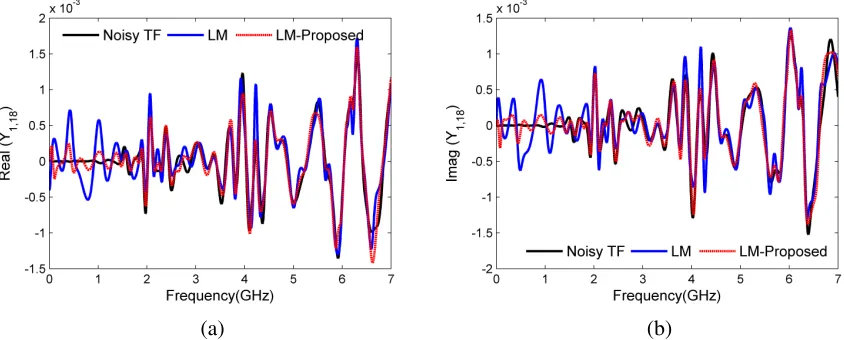
(a) (b)
Figure 3.3: Rational Approximation of the 18-dB SNR data using Noisy Eigenvectors (blue) and Actual (Noise-free) Eigenvectors (red). (a) Real part and (b) Imaginary part plots (Example 1).
This realization is different from equation (3.9). From Figure 3.3, we can see two approxi-mations, one by using eigenvectors from the actual (noise-free) data and other one from noisy
data. We can get a better approximation of the LM model by using eigenvectors from actual
data. As mentioned above, noise part in ˜WR, ˜UR, ˜LR,σL˜Rmatrices have expected mean values
of zero due to noise, these matrices do not statistically bias the results of LM approximation.
3.3.2
Eigenvector Correction from Noisy Data
In reality we do not have the noise free data to get the actual eigenvectors. Thus we are
proposing an algorithm to use the eigenvectors from previous Loewner method approximated
data to reduce the noise in the eigenvectors. Though this data is biased, it has comparatively
less noise in it after first approximation. As a result, Loewner and shifted Loewner matrices
formed by approximated data will have less noise in them. As eigenvectors are too sensitive to
SVD change of Loewner matrices, eigenvectors created from approximated data is closer to the
actual or noise-free eigenvectors. We are using an iterative approach to have these less noisy
eigenvectors from previous approximation. Consequently, we can get a better approximation of
Algorithm 1Update eigenvectors from previous LM approximated data for order r
Given: {Y˜(sm),sm}where ˜Y(sm) are the measured parameters at frequency fm =
sm 2π
Output: ˆE, ˆA, ˆB, ˆC model of the system.
1: {Y˜(sm),sm} →Construct ˜LR,σL˜ R,W˜ R,U˜R using (2.24)-(2.27) 2: [ ˜Y,Σ˜,X˜]=svd(sL˜R−σ˜LR).
3: Y˜1 =Y˜(:,1 :r), ˜X1 =X˜(:,1 :r).
4: E˜ ←Y˜∗
1L˜RX˜1,A˜ ←Y˜ ∗
1σ˜LRX˜1,B˜ ←Y˜ ∗
1U˜R,C˜ ← −W˜ RX˜1.
5: Y˜1(s)←C˜(sE˜ −A˜)−1B˜
6: {Y˜1(sm),sm} →ConstructLRΨ,σLRΨ,WRΨ,URΨusing (2.24)-(2.27) 7: [YΨ,ΣΨ,XΨ]=svd(sLRΨ−σLRΨ).
8: YΨ1 =YΨ(:,1 :r),XΨ1 =XΨ(:,1 :r).
9: Eˆ←Y∗
Ψ1L˜RXΨ1, ˆA←Y ∗
Ψ1σ˜LRXΨ1, ˆB←Y ∗
Ψ1U˜R, ˆC←−W˜ RXΨ1.
10: Y˜2(s)=Cˆ(sEˆ −Aˆ)−1Bˆ
11: Update ˜Y1(s)←Y˜2(s), goto step 6 and repeat 6-11 until convergence.
12: Update ˜Y1(s)←Y˜2(s), goto step 6 and repeat 6-9 to get the output Loewner model matrices.
3.3.3
Description of Proposed Method with LM
After the first approximation, we got ˜E, ˜A, ˜Band ˜Cmatrices mentioned in equation (3.9). Then we create our first approximated data as,
˜
Y1(s)=C˜(sE˜−A˜)−1B˜ (3.11)
Our first approximated data becomes,
˜
Y1(sm)=Y(sm)+ Ψ(sm) (3.12)
whereΨ is the error in the first approximation of noisy data ˜Y(s). Here Ψ is less noisy than
andΨis not zero-mean random noise (meaning expected mean value is not equal to zero as
E[Ψ], 0)
matrix ˜WΨand complex left data matrix ˜UΨ. They are expressed as,
˜
WΨ =W+HWΨ
˜
UΨ =U+HUΨ
(3.13)
HWΨandHUΨare noise terms due toΨin first approximated data ˜Y
1. Expected mean values of HWΨandHUΨare not zero asΨis not zero-mean randon noise.
E[HWΨ], 0 E[HWΨ]
, 0
(3.14)
From ˜WΨand ˜UΨmatrices we createWRΨ, URΨ,LRΨ andσLRΨ matrices following equation
(2.25) to (2.27) and can be expressed as,
WRΨ =WR+HWRΨ
URΨ= UR+HURΨ
LRΨ= LR+HURΨ+HWRΨ σLRΨ= σLR+HURΨ+HWRΨ
(3.15)
HereWRΨ,URΨ,LRΨandσLRΨmatrices are real right data biased matrix, real left data biased
matrix, real biased Loewner matrix and real biased shifted Loewner matrix, respectively. Here
HWRΨ andHURΨ matrices are the biased terms. Expected mean values ofHWRΨ andHURΨ are
also not zero becauseΨis not a zero-mean randon noise.
E[HWRΨ]
,0
E[HURΨ]
,0
(3.16)
The expected mean values of the biased terms present inWRΨ,URΨ,LRΨandσLRΨmatrices
from equation (3.5) due to zero-mean random noise terms present in them. However, LRΨ
andσLRΨmatrices were used to get less noisy eigenvectors, because they have less noise due
to noiseΨ.
From the SVD of (sLRΨ−σLRΨ) matrix we getYΨ&XΨmatrices.
S V D(sLRΨ−σLRΨ)= YΨΣΨXΨ (3.17)
YΨ&XΨare left and right noisy eigenvectors of the first approximated data. From the first r
columns ofYΨ&XΨ, we createYΨ1andXΨ1matrices as,
YΨ1= Y1+Y1URΨ+YW1 RΨ XΨ1 =X1+X1URΨ+XW1 RΨ
(3.18)
Here YURΨ 1 , Y
WRΨ
1 , X
URΨ
1 and X
WRΨ
1 matrices are noise terms and expected mean values of
these matrices are not zero.
AgainYURΨ 1 ,Y
WRΨ
1 ,X
URΨ
1 andX
WRΨ
1 matrices are less noisy thanY
UR 1 ,Y
WR 1 ,X
UR
1 andX
WR 1
matrices becauseΨhas less noise in it than. As a result,YΨ1 andXΨ1 eigenvectors have less
noise in it than ˜Y1and ˜X1 eigenvectors. Therefore, for our second approximation we useYΨ1
and XΨ1 eigenvectors instead of ˜Y1 and ˜X1 eigenvectors. The realization of matrices using
eigenvectors from first approximated data can be defined as,
ˆ
E =Y∗Ψ1L˜RXΨ1;
ˆ
A= YΨ∗1σL˜ RXΨ1;
ˆ
B= Y∗Ψ1U˜R;
ˆ
C =−W˜ RXΨ1;
(3.19)
Using these matrices from equation (3.19) we get our second approximation as,
˜
Y2(s)=Cˆ(sEˆ−Aˆ)
To make an iteration of this method, we update the data value of ˜Y1(s) from ˜Y2(s) data and
repeat this method for a selected order until convergence. This proposed approach will yield
more accurate result than LM solution of (3.11).
3.3.4
Methodology to Construct Previous Approximations with LM
Algorithm 1 describes the procedure to construct the less noisy eigenvectors to remove noise
from the measured data and the procedure to extract a model from the given data.
Figure 3.4: RMS error vs. order (Example 1) SNR=18dB
Figure 3.5: Proposed RMS error vs. order (Example 1) SNR=18dB.
Figure 3.6: RMS error vs. order (Example 1) SNR=16dB.
3.3.5
Order Selection
In Loewner Matrix modeling, an order is selected for model order reduction of the system. This
order of the system can be identified from the Singular Value Decomposition (SVD) drop of
Loewner Matrix [29]. When there is noise present in the data, SVD of the Loewner matrices is
contaminated and order of the system is hard to calculate from the SVD drop of LM. Therefore,
we have used LM approximated model RMS error/ H2error vs. order as our reference graph
to select the order of the system. From LM approximated model RMS error/H2error vs. order
graph we pick a range of orders. In case of Example 1 the range is from 15 to 21 shown in
Figure 3.4 for SNR=18 dB. Then for all these orders we apply our proposed algorithm. From Figure 3.5, representing proposed RMS error vs. order graph, we can see for order 17 the error
is lowest. And thus order 17 was chosen for Example 1 in case of SNR=18dB. For SNR=16dB the range of order is selected from 12 to 25 in Figure 3.6 showing LM approximated model
RMS error vs. order of the system. After applying our proposed algorithm for these range of
order values, the lowest error occurred at order 19 shown in Figure 3.7.
3.4
Numerical Examples
Four numerical examples are provided in this section to demonstrate the accuracy of the
pro-posed iterative LM method for the noisy frequency data. In the controlled experiments is the
added random noise [12, 17] and is defined as,
(sm)=Y(sm)×10−S NR/10×(Nr+ jNi) (3.21)
HereNr& Ni are real and imaginary random Gaussian noise. The noise level can be changed
Table 3.1: Poles and Residues of the TF (Example 1)
Poles (GHz) (pk) Residues (GHz) (rk) -0.6132±3.4551i -0.9877∓0.0809i -0.3940±7.3758i -0.2067∓0.0131i -0.0880±14.3024i -0.1382∓0.0145i -0.4097±17.7864i -0.1182∓0.0166i -0.2991±28.4622i -0.2426∓0.0145i -0.6447±35.2669i -0.4043∓0.0297i -1.0135±37.9655i -0.6787∓0.1465i -0.5711±57.4748i -0.2626∓0.1037i
d=0.980
3.4.1
Example 1
The first example is a synthetic transfer function (TF) with 16 poles are described in Table 3.1
is from [35]. Here 18 dB and 16 dB signal-to-noise ratios (SNRs) are considered.
(a) (b)
Figure 3.8: Rational Approximation of the 18-dB SNR data using LM and LM-Proposed ap-proximation. (a) Real part and (b) Imaginary part plots (Example 1).
Case 1:
Figure 3.8 shows the sample response of the TF with 18 dB SNR, TF from Loewner
Figure 3.9: Normalized SVD versus Order (Example 1).
Figure 3.10: RMS error vs. iteration count for SNR=18 dB (Example 1).
The LM algorithm is not able to catch the poles of the system due to biasing from the model
approximation, while the proposed method to use the eigenvectors from the previous
approx-imation iteratively shows good agreement with the original TF. Here order was found 17 to
approximate the previous LM model.
The SVD of actual (noise-free) data, noisy data and proposed method data are shown in Figure
3.9. Figure 3.10 shows the root mean square (rms) error versus iteration number, calculated as
RMS error =
v u t
1
Ns Ns
X
j=1
||Y(sj)−Yapp(sj)||2 (3.22)
whereY(sj) is equal to noisy TF andYapp(sj) corresponds to approximated TF. The rms error
for LM is 0.1032, while the rms error of LM-proposed is 0.01991 at tenth iteration.
Table 3.2 shows that the proposed iterative algorithm matches the poles of the original system
to within 0.0764%, while LM algorithm missed the pole at -0.3940 ± 7.3758. Figure 3.11 illustrates logarithmic RMS error vs. frequency plots for actual (noise-free) data LM
Figure 3.11: Log10(RMS error) vs. frequency plots for actual (noise-free) data approximation with LM (black), noisy data approximation with LM (blue) and noisy data approximation with LM-proposed (red) (Example 1)
(a) (b)
Table 3.2: Calculated Poles Using LM and proposed method (Example 1) (SNR=18 dB)
LM LM-Proposed
Poles (GHz) Error Poles (GHz) Error
-0.5440±3.4970i 2.31% -0.6123±3.4556i 0.0285% -57.9609±75.6642i 1209.2% -0.3922±7.3793i 0.0534% -0.0803±14.2929i 0.085% -0.0876±14.3026i 0.0029% -0.2563±16.6408i 0.64% -0.3973±17.7809i 0.0764% -0.3035±28.3783i 0.29% -0.2992±28.4618i 0.0013% -0.8762±35.0419i 0.91% -0.6387±35.2633i 0.0199% -0.7672±37.7031i 0.94% -1.0142±37.9710i 0.0145% -0.8999±57.4897i 0.57% -0.5720±57.4780i 0.0058%
Table 3.3: Calculated Poles Using LM and proposed method (Example 1) (SNR=16 dB)
LM LM-Proposed
Poles (GHz) Error Poles (GHz) Error
Missed pole N/A -0.6102±3.4071i 1.3707% Missed pole N/A Missed pole N/A -0.0727±14.2661i 0.2752% -0.0822±14.3026i 0.0406%
Missed pole N/A Missed pole N/A -0.4927±28.3885i 0.7279% -0.2675±28.4702i 0.1147% -1.4391±35.4639i 2.3203% -0.5848±35.1600i 0.3473% -1.0001±37.1711i 2.0920% -0.9123±38.1052i 0.4541% -1.0039±57.6811i 0.8341% -0.5498±57.3972i 0.14%
Table 3.4: 100 simulations with different random noise (Example 1) Example 1 order LM average error LM-proposed average error
18 dB 17 0.0813 0.0362
16 dB 19 0.0503 0.0297
Case 2:
Figure 3.12 shows the sample response of the TF with 16 dB SNR, TF from Loewner modeling
Here order 17 was used to approximate the previous LM model. Table 3.3 shows that LM
approximation missed three poles whereas our proposed iterative algorithm missed two poles.
To verify the proposed algorithm, 100 simulations are performed with 18dB and 16dB SNRs
with different random noise added to the TF. The average RMS error for LM and proposed iterative LM method are given in Table 3.4.
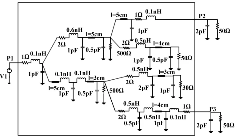
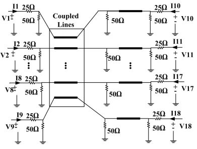
Figure 3.13: Transmission line network (Example 2)
3.4.2
Example 2
A transmission-line network is shown in Figure 3.13. The per-unit-length parameters of each
line areR= 8.26Ω/m, L = 361nH/m,C = 140pF/m, andG = 0.0S/m, and the length of the lines are listed in Figure 3.13. The Y-parameters of the three-port circuit described by the box
of Figure 3.13 is calculated at 1000 frequency points distributed evenly between 0-10 GHz and
treated as tabulated data. The data was generated using HSPICE. In this example, the added
Figure 3.14: log10 (H2error) vs order for SNR=25dB (Example 2)
Figure 3.15: Normalized Singular Values (Example 2)
(a) (b)
Figure 3.16: Rational Approximation of Y(1,3) (Example 2)(SNR=25dB).
Case 1:
(a) (b)
Figure 3.17: Rational Approximation of Y(2,3) (Example 2) (SNR=25dB).
(a) (b)
Figure 3.18: Rational Approximation of Y(2,2) (Example 2) (SNR=25dB).
has been applied and order of the system is found 105. After choosing an order 105 normalized
singular values are changed like Figure 3.15. Rational approximation of Y(1,3), Y(2,3) &
Y(2,2) are shown is Figure 3.16, 3.17, 3.18 respectively. Figure 3.19 shows RMS error vs.
iteration count for Y(1,3), Y(2,3) & Y(2,2). Figure 3.20 depictsH2error vs. iteration count for
SNR=25dB for Example 2. H2-norm error of the system is calculated as follows:
H2error=
v tPN
s
k=1||Yapp(sk)−Y(sk)|| 2 F
PNs
k=1||Y(sk)|| 2 F
Figure 3.19: RMS error versus iteration count for SNR=25 dB (Example 2).
Figure 3.20: H2-norm error versus iteration
count for SNR=25 dB (Example 2)
Figure 3.21: LM approximation of actual/noise-free data (black), LM approximation with noisy data (Blue) and proposed method approximation (Red) for order 105 (Example 2) (SNR=25dB)
(a) (b)
Figure 3.22: Rational Approximation of Y(1,3) (Example 2) (SNR=20dB)
(a) (b)
Figure 3.23: Rational Approximation of Y(2, 3) (Example 2) (SNR=20dB).
using the following equation at each frequency point,
H2 error(sk)= s
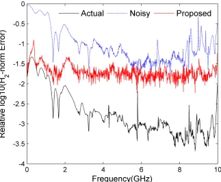
||Yapp(sk)−Y(sk)||2F
||Y(sk)||2F