Spatial interpolation using areal features: a review of methods and opportunities using new forms of data with coded illustrations

A R T I C L E

Spatial interpolation using areal features: A review

of methods and opportunities using new forms of

data with coded illustrations

Alexis Comber

| Wen Zeng

1

School of Geography, University of Leeds, UK

2

College of Geomatics, Shandong University of Science and Technology, China

Correspondence

Alexis Comber and Wen Zeng, College of Geomatics, Shandong University of Science and Technology, Qingdao, 266590, China. Email: [email protected]; alvin_z@163. com

Funding information

Natural Environment Research Council, Grant/Award Number: NE/S009124/1; State Scholarship Fund of China Scholarship Council; Natural Science Foundation of Shandong Province, Grant/Award Number: ZR201702170310

Abstract

This paper provides a high-level review of different

approaches for spatial interpolation using areal features. It

groups these into those that use ancillary data to constrain

or guide the interpolation (dasymetric, statistical,

street-weighted, and point-based), and those do not but instead

develop and refine allocation procedures (area to point,

pycnophylactic, and areal weighting). Each approach is

illus-trated by being applied to the same case study. The analysis

is extended to examine the opportunities arising from the

many new forms of spatial data that are generated by

everyday activities such as social media, check-ins, websites

offering services, microblogging sites, and social sensing, as

well as intentional VGI activities, both supported by

ubiqui-tous web- and GPS-enabled technologies. Here, data of

res-idential properties from a commercial website was used as

ancillary data. Overall, the interpolations using many of the

new forms of data perform as well as traditional, formal

data, highlighting the analytical opportunities as ancillary

information for spatial interpolation, and for supporting

spa-tial analysis more generally. However, the case study also

highlighted the need to consider the completeness and

rep-resentativeness of such data. The R code used to generate

the data, to develop the analysis and to create the tables

and figures is provided.

DOI: 10.1111/gec3.12465

This is an open access article under the terms of the Creative Commons Attribution License, which permits use, distribution and reproduction in any medium, provided the original work is properly cited.

© 2019 The Authors Geography Compass Published by John Wiley & Sons Ltd

Geography Compass.2019;13:e12465. wileyonlinelibrary.com/journal/gec3 1 of 23

K E Y W O R D S

geocomputation, population, spatial analysis, spatial analytics

1

|

I N T R O D U C T I O N

Spatial interpolation is a widely applied method in geographical research. It is a technique which uses sample values

of known geographical points (or area units) to estimate (or predict) values at other unknown points (or area units). It

has been applied to spatial data of different geographical phenomena population, hydrology, atmosphere,

topogra-phy, agriculture, soil, land use, rainfall, and temperature (Comber, Proctor, & Anthony, 2008; Goovaerts, 2000; Jia &

Gaughan, 2016; Joseph, Sharif, Sunil, & Alamgir, 2013; Liao, Li, & Zhang, 2018; Mennis, 2003; Rigol, Jarvis, & Stuart,

2001; Shi & Tian, 2006). Spatial interpolation is able to generate estimates of values at finer resolutions than the

original data. This is useful when fine scale data are unavailable or restricted to confidentiality or political reasons,

for example.

Methodological refinements have been proposed to improve spatial interpolation, focussing on ever more

sensi-tive allocation procedures (e.g., Tobler, 1979) or allocation constraints (e.g., Mennis, 2009). The latter informs the

estimations using ancillary information to mask out or guide the allocation. It has been subject to greater

develop-ment, particularly in census geography, mostly driven by changing census reporting boundaries as well as the

increased availability and variety of spatial data and by the increased functionality of GIS technologies. Some recent

research has used some of many new sources of data as ancillary information from websites, portals, social media,

check-ins, point of interest data, volunteered geographic information, and geo-tagged microblogs. These have been

driven by the increased use (and even ubiquity) of web, mobile, and GPS-enabled technologies. This paper reviews

the major developments in spatial interpolation using areal features and considers future directions afforded by such

new data sources. It groups these into methods that do not use any ancillary information (e.g., simple areal weighting,

pycnophylactic interpolation, and area-to-point interpolation), those that do (dasymetric, street-weighting methods,

statistical and geostatistical approaches, and point-based informed approaches) and approaches using new data

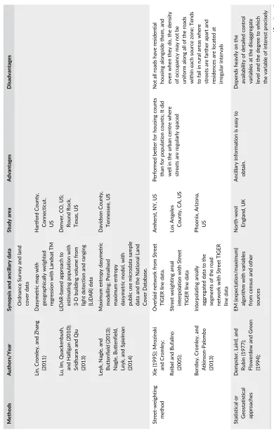
sources. Table 1 summarises the first two of these groups.

2

|

S P A T I A L I N T E R P O L A T I O N

Spatial interpolation can broadly be divided into two methods: point and areal interpolation (Lam, 1983). Point

inter-polation is used for making predictions at locations where values are unknown using other sample points that have

empirical information. Such data are typically assumed to vary continuously over space. Point interpolation

approaches include exact methods such as inverse distance weighting, kriging, and approximate methods such as

trend surface analysis (Lam, 1983). Interpolation of areal features transfers attribute information fromsourcezones

with known values to other, usually smaller but not always,targetzones with unknown values (Goodchild & Lam,

1980). The areal interpolation problem is more commonly associated with geographical analysis than other fields

(Lam, 1983). Point and areal interpolation solve very different geographic problems. In areal interpolation, the source

zones completely cover the study area, but their resolution is insufficiently fine for a particular analysis. For example,

Comber, Proctor, and Anthony (2008) transformed national agricultural land use data, recorded in source zones with

a mean area of 21 km2_{to 1 km}2_{target zones. Point interpolation constructs a surface that covers the study area}

using data recorded at a sample of locations. In geostatistics this is commonly done with kriging. Point interpolations

and geostatistics are not the subject of this paper but there is an extensive literature (see for example, Goovaerts,

TAB L E 1 Summ ary of the major ar eal interp olation a pproac hes Methods Authors/Year Synopsis and ancillary data Study area Advantages Disadvantages Simple areal weighting Goodchild and Lam (1980) Area is proportional with population London, Ontario, Canada Simple; No need of auxiliary information The homogeneity assumption, that the census population distributed evenly within a source zone, is a variation of the ecological fallacy; There is a possibility that the area selected from the source zone has a different population density than the average population density of the source zone Pycnophylactic interpolation Tobler (1979) Smooth pycnophylactic interpolation Ann Arbor, MI, US Generates a smooth surface; The total volume of each census division be preserved on the interpolated surface Unlike topography, population is not a continuously observed phenomenon Area-to-point

interpolation without ancillary information

illustrations can be found in Diggle (1983) and in Brunsdon and Comber (2018). Over the last three decades, various

approaches for areal interpolation have been developed based on different assumptions about the underlying

distri-bution of the variables to be interpolated, for example, densities or counts. These can be grouped into two broad

cat-egories: methods that use ancillary (or auxiliary) data to control, inform, guide, and constrain the reallocation process

from source to target zones, and methods that do not, but instead rely solely on the target and source zone

proper-ties (Hawley & Moellering, 2005; Langford, 2006; Zhang & Qiu, 2011).

2.1

|

Areal interpolation without ancillary information

There are three basic approaches for transforming source zones values to target zone values using the properties of

the source and target zones alone: those based on some measure of proportionality such as area (areal weighting),

those also seek to smooth the allocation to target zones to minimise discontinuities between adjacent zones

(pycnophylactic interpolation), and those that seek to take advantage of the ability of point based, geostatistical

methods to create continuous surfaces (area-to-point interpolation).

2.1.1

|

Areal weighting

Choices for areal interpolation are limited if the source zones and their attributes are the only information available.

In this situation, simple methods may be used, the best-known method of which is the area-weighting approach. This

allocates the source zone attributes proportionately to the target zones based on the area of their

inter-section (Goodchild & Lam, 1980; Lam, 1983). Area weighting is inherently volume preserving_—that is the source

zone values are maintained if the target zone values within the source zone are summed—and is easily implemented

using polygon overlay operations. Thus, the method is incorporated into most GIS software packages (Xie, 1995) and

is widely used in practice (Langford, 2006). Recent examples of research using this approach includes an examination

of methods to overcome changes in census boundary structures (Logan, Xu, & Stults, 2014) and the interpolation of

election results to new target zones (Goplerud, 2016). Goplerud (2016) noted that the method worked well when

interpolating election results across boundary changes for six different countries, with mean absolute errors in the

range of 2% to 3%. The disadvantage of this method is obvious: it assumes the relationship between the source zone

attribute being interpolated and the target zone areas to be spatially homogenous (Goodchild & Lam, 1980), an

assumption that is rarely true in the real world. However, in the absence of ancillary data, it remains a reasonable

solution (Xie, 1995; Tapp, 2010).

2.1.2

|

Pycnophylactic interpolation

Pycnophylactic interpolation was first proposed by Tobler (1979) and takes a slightly different approach to areal

weighting.

It iteratively interpolates the source zone attribute to the target zones in order to avoid sharp discontinuities

between neighbouring target zones aims, whilst preserving the overall mass or volume of the counts in the source

zones. It is a process that seeks to generate a smooth surface in the target zones from polygon-based source zones

to avoid sharp attribute discontinuities between neighbouring target zones, which are frequently raster cells. Each

iteration tries to improve the smoothness of adjacent target zone values across study area by adjusting the allocation

to each target zone, whilst preserving the target zone total (also referred to as mass or volume), using the weighted

average of target zone nearest neighbours. The number of nearest neighbours used and the number of iterations

determines the overall level of smoothing and is a subjective process (Hay, Noor, Nelson, & Tatem, 2005).

Pycnophylactic interpolation is an elegant solution to the problem of generating a continuous surface from

discontin-uous data, although it does assume that no sharp boundaries exist in the distribution of the data (Hay et al., 2005),

railways, roads) or are adjacent to waterbodies. In these cases, sharp discontinuities might be expected (for example,

in popular riverside developments). However, pycnophylactic interpolation is an elegant method and has been

adopted in many applications (Kounadi, Ristea, Leitner, & Langford, 2018; Monteiro, Martins, & Pires, 2018) as well

as in hybrid approaches (Comber, Proctor, & Anthony, 2008).

2.1.3

|

Area-to-point interpolation

A third type of areal interpolation is point-based areal interpolation (Bracken & Martin, 1989; Martin, 1989), an

extension of point interpolation (Bracken & Martin, 1989; Lam, 1983; Xie, 1995). A control point for each source

zone is identified (usually the centroid) and a density value is assigned to that point. The value is interpolated to a

regular grid of points using one of the point interpolation methods such as kriging or inverse distance weighting

(Martin, 1989; Xie, 1995). Then, the density value for each grid cell is converted back to a count and the count

values are summed over the intersecting target zones. Lam (1983) noted that the resulting target zone values

depend greatly on the choice of the control point, which has a significant impact on the grid surface. In some cases,

the source zone geometric centroid may be outside the source zone boundary, generating a questionable result

(Xie, 1995; Tapp, 2010). In others, the centroid location may adequately describe the distribution within the source

zone, which may be better described using a population-weighted centroid (Martin, 1989), for example. A further

problem is that point-based interpolators are not volume preserving and need to be rescaled (Bentley et al., 2013).

To solve this problem, Martin (1996) modified the original centroid-based algorithm to ensure that the populations

reported for target zones are constrained to match the overall sum of the source zones. Recent examples of

appli-cations using area-to-point approaches include downscaling climate models outputs (Poggio & Gimona, 2015),

urban data modelling (Anda, Erath, & Fourie, 2017), and handling mobile data streams (Kaiser & Pozdnoukhov,

2013).

2.1.4

|

Illustration: Interpolation without ancillary information

The different areal interpolation approaches (in this section and Section 2) are illustrated using a common case study:

estimating house counts for each cell in 500 m grid from US Census tracts for New Haven, Connecticut, USA. The

census data are included within thenewhavendata in theGISToolsR package (Brunsdon & Chen, 2014), with the

tracts source zones and the 500-m grid as target zones). The interpolations were developed in R and the code and

data used to generate all the figures and results in this paper are provided in Data S1.

For interpolation without ancillary information, areal weighting was undertaken using the function in thesfR

package (Pebesma et al., 2018), pycnophylactic using thepycnoR package (Brunsdon, 2014), and bespoke code was

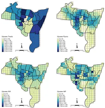
written for the area to point interpolation using inverse distance weighting. Figure 1 shows the original data with the

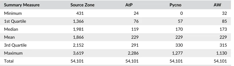
interpolation results, which are also summarised in Table 2.

Each of the three interpolation approaches shows broadly the same pattern, but with clear differences.

Consider-ing Figure 1 and Table 2 together, it is evident that the area to point estimates have higher maximum values, and

considerable spatial discontinuity between adjacent target zones. In contrast, the pycnophylactic house estimates

have lower maximum values but display a distinct poly centric pattern, with smooth but steep gradients from areas

of high population to areas with lower (even zero) population allocations. The area weighting estimates have

shallower gradients between areas with high and low allocated populations, and lower maximum values than area to

point. The median values in Table 2 characterise some of these differences.

2.2

|

Methods using ancillary information

The main problem with spatially unconstrained interpolation approaches is that they are likely to allocate source

information with some relationship to the source zone variable can be used to constrain or inform allocation to target

zones (Liu et al., 2008). Interpolations undertaken in this way can result in allocations that better reflect actual

distri-butions, because the ancillary data is closely related to the data being interpolated. Population distridistri-butions, for

example, are closely related to features such as residential land use. A number of algorithms using ancillary data have

been developed, informed by the increasing variety of different data types (Langford, 2013). These methods have

been extensively applied to population interpolations (Cromley et al., 2012; Langford, 2007; Mennis, 2003; Reibel &

Agrawal, 2007), socioeconomic variable estimations (Eicher & Brewer, 2001; Goodchild, Anselin, & Deichmann,

1993; Mennis & Hultgren, 2006), and to handle changing historical administrative boundaries (Gregory, 2002;

Mennis, 2016).

Methods for areal interpolation using ancillary data can be grouped into four sets of approaches: those which

apply areal masks to inform interpolation (dasymetric mapping), those using road networks to allocate populations

along target zone road segments (street-weighting method), those which establish a statistical relationship between

the ancillary data and the source zone data to guide allocation (statistical approaches), and those which use point

data as ancillary information (point-based approaches).

2.2.1

|

Dasymetric mapping

The dasymetric interpolation approach is the most cited of the methods that use ancillary information (Langford,

2013). Ancillary data includes areal features and linear or point features with buffers. It was first proposed as a

car-tographic technique to address some of the issues associated with choropleth mapping. Mennis (2009) provides a

comprehensive overview of the origins of the dasymetric approaches, linking back to 19th century dasymetric maps

of population (Semenov-Tian-Shansky, 1928) and the work of Wright (1936). An accessible introduction can be

found in Mennis (2003) who defines dasymetric mapping as“areal interpolation that uses ancillary (additional and

related) data to aid in the areal interpolation process_”(p32). It guides the redistribution of source zone values to

target zones using auxiliary information as a spatial control. Dasymetric approaches can either identify areas to

include/exclude from the interpolation process. Population data, for example, are excluded from nonresidential

areas. They can also highlight areas that might expected to have higher/lower population densities than others

(Cromley et al., 2012). In early work, the most commonly used ancillary information was areal masks related to land

use classified from remotely sensing data. In the 1990s, the Leicester group (David Unwin, David Maguire, Mitchel

Langford, Peter Fisher) published a series of methods papers informed by urban land use data derived from satellite

imagery. Langford and Unwin (1994) and Fisher and Langford (1996) demonstrated the improvements in areal

interpolation using dasymetric mapping as have a number of authors subsequently (Eicher & Brewer, 2001;

Langford, 2006; Mennis, 2003; Mennis & Hultgren, 2006).

The simplest dasymetric approach is to create binary masks of areas that are included or excluded from the

inter-polation process. Binary dasymetric approaches (Fisher & Langford, 1996) would, for example, exclude nonresidential

areas in target zones when interpolating population data. However, population density may vary in different land

use classes (Lin, Cromley, Civco, Hanink, & Zhang, 2013). Categorical dasymetric approaches assign different

propor-tions of the total population to different land classes (Eicher & Brewer, 2001) or select target zones that are

homoge-neous with regard to a specified land class (Mennis, 2003). Mennis and Hultgren (2006) extended this further by

applying proportion thresholds to target zone land use categories, and Yuan et al. (1997) developed a model that

regressed population over different land use types to quantify the relationships between population and land use

classes. Langford (2006) argued that dividing the study area into subregions to fit the local regression model has little

relationship with population distributions, and Lin et al. (2011) applied a geographically weighted regression to model

variations in the relationship between population density and land use type.

Other kinds of mapped data have been used. Moon and Farmer (2001) manually digitised ancillary data and

Langford (2007) experimented with information derived from raster pixel maps. Dasymetric approaches have been

extended with a range of different data inputs, including cadastral data (Maantay et al., 2007; Tapp, 2010), LiDAR

data (Lu et al., 2010; Sridharan & Qiu, 2013) which have been found to improve the accuracy of population

estima-tion. Comber, Proctor, and Anthony (2008) combined dasymetric and pycnophylactic approaches to create a national T A B L E 2 Summaries of the distributions of the house estimates from the different approaches

Summary Measure Source Zone AtP Pycno AW

Minimum 431 24 0 32

1st Quartile 1,366 76 57 85

Median 1,981 119 170 173

Mean 1,866 229 229 229

3rd Quartile 2,152 291 330 315

Maximum 3,619 2,286 1,277 1,130

Total 54,101 54,101 54,101 54,101

agricultural land use dataset in the United Kingdom using Ordnance Survey data to mask out nonagricultural features

(urban and woodland areas, buffered rivers and roads). Lu et al. (2010) and Sridharan and Qiu (2013) used LiDAR

data to estimate populations at building level. Leyk et al. (2013) developed a maximum entropy dasymetric model

using USGS national land cover data and multiple attributes from the population census to generate correlations

between ancillary variables and population. Nagle et al. (2014) extended this to incorporate uncertainty into the

modelling process.

There are a number of potential problems with dasymetric approaches. First, the performance of any given

dasymetric approach has been found to vary substantially in different study areas, with no single technique

consis-tently outperforming all others (Zandbergen & Ignizio, 2010). Second, although dasymetric mapping can provide a

more spatially informed interpolation, the implementation of such approaches imposes greater demands in terms of

ancillary data requirements (Cromley et al., 2012). Auxiliary information is often derived from remote sensing images

or land use data, which are not always available (Sadahiro, 2000), especially in developing countries (Yang, Jiang,

Luo, & Zheng, 2012). Further, the increases in computational costs can limit the wider applicability of methods as

large quantities of polygons, raster cells, or both have to be processed (Zhang & Qiu, 2011). Dasymetric approaches

using remote sensing data also requires an understanding of multispectral signatures, image classification techniques,

etc. that may be outside the analyst's skill set (Langford, 2013). They also assume population density to be

homoge-neous in each land use class whether binary or using categorical masks. Fourth, they are inherently subject to the

ecological fallacy or modifiable areal unit problem (MAUP, Openshaw, 1984) and can generate different results

depending on the scales of target and source zones. Finally, with any dasymetric approach, the quality and relevance

of the ancillary data and any intrinsic relationships with the source zones has a critical influence on the

representa-tiveness of the target zone estimates.

2.2.2

|

Street-weighting method

The street-weighting method (Xie, 1995) uses street network data. Several variants of the methodology exist, the

simplest of which uses the network length within the source zone and distributes population uniformly along street

segments within its boundaries. The linear features are then intersected with the target zones and an estimated

pop-ulation count is derived by summing the poppop-ulation along each road segment within the target zone boundary. Reibel

and Bufalino (2005) tested Xie's algorithm and showed it to be more accurate than simple area weighting. A

signifi-cant difference between areal and street weighting is the way that the weighting is applied. In areal weighting,

inter-secting areas drives the allocation. In street-weighting this is done by the length of the interinter-secting linear objects.

This approach performs well in urban areas, with regularly spaced streets, but has been found to underperform in

rural areas with fewer streets and residences located at irregular intervals on them (Tapp et al., 2010).

2.2.3

|

Statistical and geostatistical methods

Statistical areal interpolation methods use ancillary data in conjunction with statistical techniques to establish

func-tional relationships between the spatial distribution of the ancillary data and the spatial distribution of source zone

data to be interpolated (Flowerdew & Green, 1991; Goodchild et al., 1993; Reibel & Agrawal, 2007; Lin, Cromley, &

Zhang, 2011). A regression analysis is usually conducted at the source zone level to model the variable of interest

from other source zone attributes. The resulting model is then applied to each target zone to predict values using

tar-get zone attributes. Some refinements to this approach have been proposed. Flowerdew and Green (1991, 1994)

used an expectation/maximum (EM) algorithm (Dempster et al., 1977) to model relationships between population

density and socioeconomic variables. Harvey (2002) applied an iterated regression procedure as a least-squares

approximation of the EM algorithm to model population from satellite image pixels classified as residential. Statistical

methods typically generate a model which is then uniformly applied to target zones across the whole study area (Xie,

regression approach to provide estimates conditioned on local parameters rather than global ones and Schroeder

and Van Riper (2013) developed a geographically-weighted EM algorithm. This allowed the allocation to target zones

to vary spatially, depending on the local model coefficient estimates for the various land use categories related to

built-up areas. The major factor with the use of such statistical approaches is that they depend heavily on the

avail-ability of detailed control variables (such as residential land use) at the target zone level and on the assumption that

the variable of interest follows a known or quantifiable statistical distribution, which can limit their wider application

(Zhang & Qiu, 2011).

Geostatistical interpolation methods were originally designed for point interpolation and have been applied in

areal interpolation because of their ability to accommodate spatial autocorrelation into the modelling process.

Kyriakidis (2004) established a theoretical framework for interpolation based on spatial cross-correlation between

areal and point variables using cokriging. Kyriakidis and Yoo (2005) applied this approach to a synthetic image

dataset. Wu and Murray (2005) developed a cokriging areal interpolation approach with pixel level variance

estima-tions from the impervious surface fraction representing roads, roofs, etc. Liu et al. (2008) further extended this model

to disaggregate the residuals from the regression of population density with built-up and vegetation compositions

and Meng et al. (2013) combined multivariate regression with kriging to improve spatial prediction accuracy for

weakly correlated auxiliary variables. Geostatistical methods are inherently pycnophylactic—they preserve volume

and handle process spatial heterogeneity_—but Griffith (2013) noted that kriging and cokriging involve variable

trans-formation which may introduce errors in final population estimates. However, geostatistical-based areal interpolation

is an emerging approach whose theoretical framework has been developed and tested with applications using

simu-lated data and satellite imagery.

2.2.4

|

Point-based ancillary information

Areal interpolation approaches with point-based information use the point locations to guide the interpolation to

tar-get zones (Zhang & Qiu, 2011). Tapp (2010) used address points as ancillary information to predict population and

the results showed significant reductions in target zone estimate error compared to other methods. Harris and Chen

(2005) used post code points with the population surface modelling technique proposed by Martin (1989) and

Bracken and Martin (1989) to estimate population density. Zhang and Qiu (2011) used school locations to interpolate

population with classic density models and Langford (2013) used primary school locations and bus stop points. Point

data have a much simpler structure than polygon or line data and do not require topological information to be

deter-mined to represent spatial relationships (Zhang & Qiu, 2011). Many different types of point data are widely available

from different portals and databases, supporting the interpolation of different types of variables to target zones.

Because they represent features at discrete dimensionless locations, there is no risk of ecological fallacy or the

MAUP, in contrast to area-based ancillary information which implicitly assume even within zone distributions (Tapp,

2010). As new data sources emerge (see below), there are increased opportunities for point-based methods to

com-plement methods using polygon or line based ancillary data.

2.2.5

|

Illustration: Interpolation with ancillary information

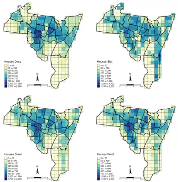
The four areal interpolation approaches using ancillary are illustrated in Figure 2 using thenewhavencensus tracts

(source zones) and the 500-m polygon grid (target zones) described above. Bespoke R code was written for each of

these analyses and to produce the maps in Figure 2 and the summaries in Table 3, provided in Data S1.

The interpolation approaches using ancillary information to constrain and guide them show broadly similar

pat-terns, but with some subtle differences. Considering Figure 2 and Table 3, two characteristics stand out. First, the

negative values and flatter distribution of the estimates from the statistical approach. This is to be expected: a simple

linear regression model was constructed then used to predict target zone house counts. One of the model coefficient

F I G U R E 2 The interpolation results for approaches using ancillary data (Dasy, dasymetric; Street, street-weighted; Stat = statistical; Point = point-based)

T A B L E 3 Summaries of the distributions of the house estimates from the interpolation approaches using ancillary information

Summary Measure Dasy Stat Street Point

Minimum 0 -1432 0 0

First Quartile 44 64 45 27

Median 168 230 198 167

Mean 229 229 229 229

Third Quartile 331 418 334 361

Maximum 1,440 775 1,101 1,313

Total 54,101 54,101 54,101 54,101

predictor variables) with the result that the predictions for some areas inevitably will be negative. The second striking

feature is the high degree of degree of homogeneity in spatial distributions of the other three approaches—there are

similar patterns of discontinuity and gradients between high and low target zone areas. This indicates a generic

bene-fit of the inclusion ofsome kindof relevant additional information to guide the interpolation. Their statistical

distribu-tions are similar to the pycnophylactic and areal weighting approaches (Figure 1, Table 2).

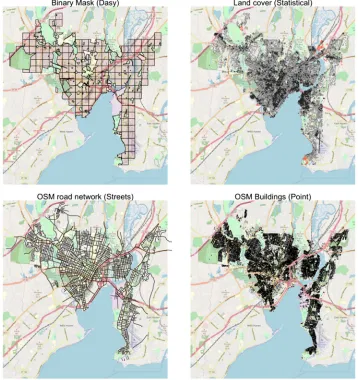
The ancillary data used in the different interpolations (with the outline methods) were as follows:

• Dasymetric: Parks data from the City of New Haven data portal, plus features labelled as_“land use,_{” “}amenity,_” and_“coastline_” extracted from OpenStreetMap to mask these areas out. This was used as input to an areal

weighting approach.

• Street weighted: road linear features were extracted from OpenStreetMap. The proportion of the source zone streets in each target zone was determined and used to allocate house estimates.

• Statistical: data from the 2011 National Land Cover Dataset was downloaded from the USGS portal. Three land use classes were used to train a linear regression model: Developed, High Intensity, Developed, Medium Intensity,

and Grassland/Herbaceous. Counts of these were created over source zones and target zones. The model was

trained over source zone counts and then used to predict houses over target zones.

• Point-based: features labelled with_“building_”were extracted from OpenStreetMap. The proportion of the source zone buildings in each target zone was determined and used to allocate house estimates.

The ancillary data are shown in Figure 3 and full details of how they were obtained (including the code for

extracting them), manipulated, and applied in the area interpolations are fully detailed in Data S1.

3

|

N E W F O R M S O F D A T A

Interpolation approaches using ancillary data generate more accurate results than approaches that do not include

such data, although with some questions about their generalisability (e.g., Zandbergen & Ignizio, 2010). Remotely

sensed imagery, road network, and land use/cover are the most commonly used ancillary data for interpolating

popu-lation (Lin & Cromley, 2015). However, ancillary data can be expensive or unavailable. To overcome this, approaches

have been developed that use the many new forms data as ancillary data. For example, in developing countries,

especially rural areas, high-resolution spatial datasets are rarely available. Some research has used Google Earth

imagery to extract auxiliary information (Yang et al., 2012), taxation data (Jia & Gaughan, 2016; Kar & Hodgson,

2012), and social media data (Yu, Li, Zhu, & Plaza, 2018). New forms of data able to support spatial interpolation are

available from three general sources as follows:

1. Open data initiatives, from national mapping agencies, local government data portals (Benitez-Paez, Comber,

Tri-lles, & Huerta, 2018) to community-led open data infrastructures such as the Open Data Institute (https://

theodi.org), and the many academic research led data centres, such as the CDRC (https://www.cdrc.ac.uk) in the

UK (Vij, 2016);

2. Online service providers, particularly property sales and rentals for population interpolation, but also

commer-cially produced but freely available Point-Of-Interest (POI) data; and

3. Data generated by citizens through social media posts, check-ins as well as citizen sensing and volunteered

geo-graphic information (VGI) activities such as OpenStreetMap, supported by mobile personal devices with

web-and GPS-enabled technologies.

There is necessarily some overlap between the groups. For example, social media check-ins are frequently to

created and collected as part of our everyday lives with location attached (all data are spatial now), and the ease with

which data are uploaded and shared via open and queriable repositories.

Many national mapping agencies have been forced to respond to this open data explosion: the alternative is to

lose their users but also their primacy and ultimately funding. For example, in the United Kingdom, this has resulted

in open and free access to high-quality national mapping agency data, providing highly consistent ancillary data

resources to support dasymetric interpolation (Langford, 2013). User-contributed information and VGI provide

alter-native sources of ancillary data for dasymetric interpolation, as used in a number of studies (Bakillah et al., 2014;

Kunze & Hecht, 2015; Geiß et al., 2017). Although there are potential quality issues, these provide valuable data

sources that can complement official and commercial data (Goodchild, 2007; Bakillah et al., 2014). Other geographic

data generated by social networks is also emerging as a further source of ancillary data, with for example, Lin and

to the representativeness of the sample. Their results indicated that using geo-located tweets as ancillary data did

not perform as well methods using traditional data, although for specific age groups with a high percentage of

Twit-ter users, it improved prediction. Other work has demonstrated inTwit-terpolation enhancements with mobile phone data

(Liu, Peng, Wu, Jiao, & Yu, 2018) and POI data (Ye et al., 2018) as input to dasymetric approaches. Undoubtedly, the

robustness of the interpolation depends on the choice of ancillary data, as well as the interpolation methodological

approach.

3.1

|

Illustration: Interpolation with new forms of data

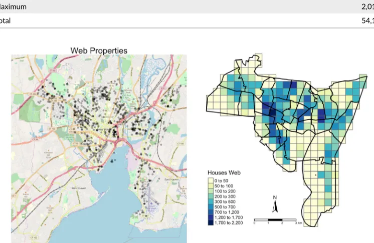
To illustrate this, property data (rentals and for sale) for New Haven were downloaded from www.zillow.com in

January 2019. Each record included the latitude and longitude of the property. Property locations were used as input

to a point-based interpolation in the same way as that described in Section 2.2. The results are shown in Figure 4

and summarised in Table 4. The details and the code used to do this are in Data S1.

The striking features of the spatial and statistical distributions of the house estimates using data from the a

prop-erty website are the large number of target zones with a house estimate of 0, the high maximum values compared to

F I G U R E 4 The locations of property for sale or rent downloaded from zillow.com (n= 926), shaded with a transparency term (© OpenStreetMap contributors), and point-based interpolation estimates, informed by property counts

T A B L E 4 Summary of the distribution of the house estimates from an interpolation using ancillary property information from the web

Summary Measure Web

Minimum 0

First Quartile 0

Median 115

Mean 229

Third Quartile 353

Maximum 2,015

the results in Tables 2 and 3 and Figures 1 and 2, and the lower median values. These indicate that some of the target

zones contained no properties listed on the website from which the data was taken, with the original source zones

counts allocated to those that did. Interestingly, the spatial distribution is similar to the point based approach

(Figure 2) that used OpenStreetMap buildings point data. This reinforces the need to carefully evaluate and consider

the representativeness of many of the new forms ofinformalspatial data that are available for use in such analyses.

The OpenStreetMap data in this case is relatively complete, but similar problems of completeness and

representa-tiveness might be expected if it was used for study with poor OpenStreetMap coverage.

It is instructive to compare the results of the interpolation approaches and different ancillary data. The pair-wise

correlations, distributions, and pair-wise scatterplots of the target zone estimated populations from each of the eight

interpolations are shown in Figure 5. All of the correlations are significant and generally are in the range 0.70 to

0.95. The distributions have a broadly similar form, with a large number of lower estimates, tailing off to a smaller

number of higher ones. The exceptions are the Statistical and Area-to-Point approaches, which consequently have

the lowest correlations. This suggests that these approaches generate noticeably different predicted populations to

the others.

4

|

C O N C L U S I O N S

This paper reviews and summarises the main approaches used in spatial interpolation of areal features. It separates

these into those that include ancillary information to constrain or guide interpolation and those that do not. Each

approach was illustrated using data for the 29 census tracts in New Haven (CT). Data of household number from

thesesource zones were interpolated to a 500-m polygon grid (target zones), and ancillary data from a range of

sources ware used to constrain the interpolation including areal, linear, and point-based features. Additionally, data

of properties for sale and rent were scrapped from a commercial website and used to illustrate the potential utility of

the many new forms of data as inputs to dasymetric approaches and related interpolation algorithms.

There is ever-increasing amount of data available that could be used to support spatial analysis more

gener-ally as well as methods spatial disaggregation. For formal data, availability is being driven open access initiatives

and data portals which are opening up databases that were once the preserve of national mapping agencies

and government. The volumes of informal data are increasing as well. These are generated by the everyday

activities of citizens and businesses through social media (check-ins, etc.), websites offering services,

micro-blogging, social sensing, as well as VGI activities such as OpenStreetMap, and supported by ubiquitous

web-and GPS-enabled technologies. However, the use such data presents new challenges particularly around data

quality and the representativeness of the data relative to the process of interest (Comber, Mooney, Purves,

Rocchini, & Walz, 2016). Formal data created by national mapping agencies and served through open data

por-tals comes with assurances of quality, experimental design, metadata confirming to standards, and

documenta-tion. These are critically lacking in many new forms of data, requiring the user explicitly evaluate the suitability

of the data for their intended application (Comber, Fisher, Harvey, Gahegan, & Wadsworth, 2006; Comber,

Fisher, & Wadsworth, 2008). This paper evaluated ancillary data from a number of traditional and informal

sources to illustrate different areal interpolation methods. The case study using data from a property website

highlighted the need to consider the representativeness of such data before using it as ancillary data. However,

generally, a correlation analysis of showed that new forms of data have can perform as well as traditional data.

This indicates the opportunities afforded to include such data, with health warnings, as ancillary information for

spatial interpolation and to support spatial analysis more generally.

A C K N O W L E D G E M E N T

This work was supported by the Natural Science Foundation of Shandong Province (ZR201702170310), the

State Scholarship Fund of China Scholarship Council (201808370092), and the Natural Environment Research

Council (NE/S009124/1). All of the analyses and mapping were undertaken in R 3.5.3 the open source

statisti-cal software.

O R C I D

Alexis Comber https://orcid.org/0000-0002-3652-7846

R E F E R E N C E S

Anda, C., Erath, A., & Fourie, P. J. (2017). Transport modelling in the age of big data.International Journal of Urban Sciences,

21(sup1), 19_–42.

Bakillah, M., Liang, S., Mobasheri, A., Jokar Arsanjani, J., & Zipf, A. (2014). Fine-resolution population mapping using OpenStreetMap points-of-interest.International Journal of Geographical Information Science,28(9), 1940_–1963. https:// doi.org/10.1080/13658816.2014.909045

Benitez-Paez, F., Comber, A., Trilles, S., & Huerta, J. (2018). Creating a conceptual framework to assess and improve the

re-usability of open geographic data in cities.Paper accepted for publication in Transactions in GIS,22, 806–822. https://doi. org/10.1111/tgis.12449

Bentley, G. C., Cromley, R. G., & Atkinson-Palombo, C. (2013). The network interpolation of population for flow modeling using dasymetric mapping.Geographical Analysis,45(3), 307_–323. https://doi.org/10.1111/gean.12013

Bracken, I., & Martin, D. (1989). The generation of spatial population distributions from census centroid data.Environment and Planning A,21(4), 537_–543. https://doi.org/10.1068/a210537

Brunsdon, 2014. Pycno: Pycnophylactic Interpolation. R package version 1.2.

Brunsdon, C. and Chen, H., 2014. GISTools: Some further GIS capabilities for R. R package version 0.7-4. Brunsdon, C., & Comber, L. (2018).An introduction to R for spatial analysis and mapping (2ndedition). London: Sage.

Comber A, Mooney P, Purves RS, Rocchini D and Walz A (2016). Crowdsourcing: It matters who the crowd are. The impacts

of between group variations in recording land cover.PlosONE,11(7): e0158329, DOI: https://doi.org/10.1371/journal. pone.0158329

Comber, A., Proctor, C., & Anthony, S. (2008). The creation of a national agricultural land use dataset: Combining pycnophylactic interpolation with dasymetric mapping techniques.Transactions in GIS,12(6), 775_–791. https://doi.org/ 10.1111/j.1467-9671.2008.01130.x

Comber, A. J., Fisher, P. F., Harvey, F., Gahegan, M., & Wadsworth, R. (2006). Using metadata to link uncertainty and data

quality assessments. InProgress in Spatial Data Handling(pp. 279–292). Berlin, Heidelberg: Springer.

Comber, A. J., Fisher, P. F., & Wadsworth, R. A. (2008). Semantics, metadata, geographical information and users.

Transac-tions in GIS,12(3), 287–291. https://doi.org/10.1111/j.1467-9671.2008.01102.x

Cromley, R. G., Hanink, D. M., & Bentley, G. C. (2012). A quantile regression approach to areal interpolation.Annals of the Association of American Geographers,102(4), 763_–777. https://doi.org/10.1080/00045608.2011.627054

Dempster, A., Laird, N., & Rubin, D. (1977). Maximum likelihood from incomplete data via the EM algorithm.Journal of the Royal Statistical Society, Series B,39, 1_–38.

Diggle, P. J. (1983).Statistical analysis of spatial point patterns. London: Academic Press.

Eicher, C. L., & Brewer, C. A. (2001). Dasymetric mapping and areal interpolation: Implementation and evaluation. Cartogra-phy and Geographic Information Science,28(2), 125_–138. https://doi.org/10.1559/152304001782173727

Fisher, P. F., & Langford, M. (1996). Modeling sensitivity to accuracy in classified imagery: A study of areal interpolation by dasymetric mapping.The Professional Geographer,48(3), 299_–309. https://doi.org/10.1111/j.0033-0124.1996.00299.x Flowerdew, R., & Green, M. (1991). Data integration: Statistical methods for transferring data between zonal systems. In

I. Masser, & M. Blakemore (Eds.),Handling Geographical Information, 38_–54. London: Longman.

Flowerdew, R., & Green, M. (1994). Areal interpolation and types of data. In A. S. Fotheringham, & P. Rogerson (Eds.),Spatial Analysis and GIS(pp. 121_–145). London: Taylor and Francis.

Geiß, C., Schauß, A., Riedlinger, T., Dech, S., Zelaya, C., Guzmán, N.,_…Taubenböck, H. (2017). Joint use of remote sensing data and volunteered geographic information for exposure estimation: Evidence from Valparaíso, Chile.Natural Hazards,

86(1), 81–105. https://doi.org/10.1007/s11069-016-2663-8

Goodchild, M. F., Anselin, L., & Deichmann, U. (1993). A framework for the areal interpolation of socioeconomic data. Envi-ronment and Planning A,25(3), 383_–397. https://doi.org/10.1068/a250383

Goodchild, M. F., & Lam, N. S.-N. (1980). Areal interpolation: A variant of the traditional spatial problem.Geo-Processing,1, 297_–312.

Goovaerts, P. (1999). Geostatistics in soil science: State-of-the-art and perspectives.Geoderma,89(1-2), 1–45. https://doi. org/10.1016/S0016-7061(98)00078-0

Goovaerts, P. (2000). Geostatistical approaches for incorporating elevation into the spatial interpolation of rainfall.Journal of hydrology,228(1-2), 113_–129. https://doi.org/10.1016/S0022-1694(00)00144-X

Goplerud, M. (2016). Crossing the boundaries: An implementation of two methods for projecting data across boundary changes.Political Analysis,24(1), 121_–129. https://doi.org/10.1093/pan/mpv029

Gregory, I. N. (2002). The accuracy of areal interpolation techniques: standardising 19th and 20th century census data to

allow long-term comparisons.Computers, Environment and Urban Systems,26(4), 293–314.

Griffith, D. A. (2013). Estimating missing data values for georeferenced poisson counts. Geographical Analysis, 45(3),

Harris, R., & Chen, Z. (2005). Giving dimension to point locations: urban density profiling using population surface models.

Computers, Environment and Urban Systems,29(2), 115–132. https://doi.org/10.1016/j.compenvurbsys.2003.08.003 Harvey, J. T. (2002). Population estimation models based on individual TM pixels.Photogrammetric Engineering and Remote

Sensing,68(11), 1181–1192.

Hawley, K., & Moellering, H. (2005). A comparative analysis of areal interpolation methods.Cartography and Geographic Information Science,32(4), 411_–423. https://doi.org/10.1559/152304005775194818

Hay, S. I., Noor, A. M., Nelson, A., & Tatem, A. J. (2005). The accuracy of human population maps for public health applica-tion.Tropical Medicine & International Health,10(10), 1073_–1086. https://doi.org/10.1111/j.1365-3156.2005.01487.x Jia, P., & Gaughan, A. E. (2016). Dasymetric modeling: A hybrid approach using land cover and tax parcel data for

mapping population in Alachua County, Florida.Applied Geography, 66, 100–108. https://doi.org/10.1016/j.apgeog. 2015.11.006

Joseph, J., Sharif, H. O., Sunil, T., & Alamgir, H. (2013). Application of validation data for assessing spatial interpolation methods for 8-h ozone or other sparsely monitored constituents.Environmental Pollution,178, 411_–418. https://doi. org/10.1016/j.envpol.2013.03.035

Kaiser, C., & Pozdnoukhov, A. (2013). Enabling real-time city sensing with kernel stream oracles and MapReduce.Pervasive and Mobile Computing,9(5), 708_–721. https://doi.org/10.1016/j.pmcj.2012.11.003

Kar, B., & Hodgson, M. E. (2012). A process oriented areal interpolation technique: A coastal county example.Cartography and Geographic Information Science,39(1), 3_–16. https://doi.org/10.1559/152304063913

Kounadi, O., Ristea, A., Leitner, M., & Langford, C. (2018). Population at risk: Using areal interpolation and Twitter messages

to create population models for burglaries and robberies. Cartography and Geographic Information Science, 45(3), 205_–220. https://doi.org/10.1080/15230406.2017.1304243

Krivoruchko, K., Gribov, A., & Krause, E. (2011). Multivariate areal interpolation for continuous and count data.Procedia Environmental Sciences,3, 14_–19. https://doi.org/10.1016/j.proenv.2011.02.004

Kunze, C., & Hecht, R. (2015). Semantic enrichment of building data with volunteered geographic information to improve

mappings of dwelling units and population.Computers, Environment and Urban Systems,53, 4–18. https://doi.org/10. 1016/j.compenvurbsys.2015.04.002

Kyriakidis,P. C. (2004). A geostatistical framework for area-to-point spatial interpolation.Geographical Analysis,36(3), 259– 289. https://doi.org/10.1111/j.1538-4632.2004.tb01135.x

Kyriakidis, P. C. & Yoo, E. H. (2005). Geostatistical prediction and simulation of point values from areal data.Geographical

Analysis,37(2), 124–151.

Lam, N.S.N. (1983). Spatial interpolation methods: A review.The American Cartographer,10(2), 129_–150. https://doi.org/10. 1559/152304083783914958

Langford, M. (2006). Obtaining population estimates in non-census reporting zones: An evaluation of the 3-class dasymetric method.Computers, Environment and Urban Systems,30(2), 161_–180. https://doi.org/10.1016/j.compenvurbsys.2004. 07.001

Langford, M. (2007). Rapid facilitation of dasymetric-based population interpolation by means of raster pixel maps.

Computers, Environment and Urban Systems,31(1), 19–32. https://doi.org/10.1016/j.compenvurbsys.2005.07.005 Langford, M. (2013). An evaluation of small area population estimation techniques using open access ancillary data.

Geographical Analysis,45(3), 324_–344. https://doi.org/10.1111/gean.12012

Langford, M., & Unwin, D. J. (1994). Generating and mapping population density surfaces within a geographical information system.The Cartographic Journal,31(1), 21_–26. https://doi.org/10.1179/caj.1994.31.1.21

Leyk, S., Nagle, N. N., & Buttenfield, B. P. (2013). Maximum entropy dasymetric modeling for demographic small area

estima-tion.Geographical Analysis,45(3), 285–306. https://doi.org/10.1111/gean.12011

Li, J., & Heap, A. D. (2011). A review of comparative studies of spatial interpolation methods in environmental sciences:

performance and impact factors.Ecological Informatics,6(3-4), 228–241. https://doi.org/10.1016/j.ecoinf.2010.12.003 Liao, Y., Li, D., & Zhang, N. (2018). Comparison of interpolation models for estimating heavy metals in soils under various

spatial characteristics and sampling methods.Transactions in GIS,22(2), 409_–434. https://doi.org/10.1111/tgis.12319 Lin, J., Cromley, R., & Zhang, C. (2011). Using geographically weighted regression to solve the areal interpolation problem.

Annals of GIS,17(1), 1_–14. https://doi.org/10.1080/19475683.2010.540258

Lin, J., Cromley, R. G., Civco, D. L., Hanink, D. M., & Zhang, C. (2013). Evaluating the use of publicly available remotely

sensed land cover data for areal interpolation.GIScience & Remote Sensing,50(2), 212–230. https://doi.org/10.1080/ 15481603.2013.795304

Lin, J., & Cromley, R. G. (2015). Evaluating geo-located Twitter data as a control layer for areal interpolation of population.

Applied Geography,58, 41_–47. https://doi.org/10.1016/j.apgeog.2015.01.006

Liu, L., Peng, Z., Wu, H., Jiao, H., & Yu, Y. (2018). Exploring urban spatial feature with dasymetric mapping based on mobile

Liu, X. H., Kyriakidis, P. C., & Goodchild, M. F. (2008). Population-density estimation using regression and area-to-point residual kriging. International Journal of Geographical Information Science, 22(4), 431–447. https://doi.org/10.1080/ 13658810701492225

Logan, J. R., Xu, Z., & Stults, B. J. (2014). Interpolating US decennial census tract data from as early as 1970 to 2010: A longitudinal tract database. The Professional Geographer, 66(3), 412_–420. https://doi.org/10.1080/00330124.2014. 905156

Lu, Z., Im, J., Quackenbush, L., & Halligan, K. (2010). Population estimation based on multi-sensor data fusion.International Journal of Remote Sensing,31(21), 5587_–5604. https://doi.org/10.1080/01431161.2010.496801

Maantay, J. A., Maroko, A. R., & Herrmann, C. (2007). Mapping population distribution in the urban environment: The cadastral-based expert dasymetric system (CEDS). Cartography and Geographic Information Science, 34(2), 77–102. https://doi.org/10.1559/152304007781002190

Martin, D. (1989). Mapping population data from zone centroid locations.Transactions of the Institute of British Geographers,

14, 90_–97. https://doi.org/10.2307/622344

Martin, D. (1996). An assessment of surface and zonal models of population.International Journal of Geographical Information Systems,10(8), 973–989. https://doi.org/10.1080/02693799608902120

Meng, Q., Liu, Z., & Borders, B. E. (2013). Assessment of regression kriging for spatial interpolation_—Comparisons of seven GIS interpolation methods. Cartography and Geographic Information Science,40(1), 28_–39. https://doi.org/10.1080/ 15230406.2013.762138

Mennis, J. (2003). Generating surface models of population using dasymetric mapping.The Professional Geographer,55(1), 31_–42.

Mennis, J. (2009). Dasymetric mapping for estimating population in small areas.Geography Compass,3(2), 727_–745. https:// doi.org/10.1111/j.1749-8198.2009.00220.x

Mennis, J. (2016). Dasymetric spatiotemporal interpolation.The Professional Geographer,68(1), 92–102. https://doi.org/10. 1080/00330124.2015.1033669

Mennis, J., & Hultgren, T. (2006). Intelligent dasymetric mapping and its application to areal interpolation.Cartography and Geographic Information Science,33(3), 179–194. https://doi.org/10.1559/152304006779077309

Monteiro, J., Martins, B., & Pires, J. M. (2018). A hybrid approach for the spatial disaggregation of socio-economic indicators.

International Journal of Data Science and Analytics,5(2-3), 189_–211. https://doi.org/10.1007/s41060-017-0080-z Moon, Z. K., & Farmer, F. L. (2001). Population density surface: A new approach to an old problem.Society & Natural

Resources,14(1), 39–51. https://doi.org/10.1080/089419201300199545

Nagle, N. N., Buttenfield, B. P., Leyk, S., & Spielman, S. (2014). Dasymetric modeling and uncertainty.Annals of the Associa-tion of American Geographers,104(1), 80_–95. https://doi.org/10.1080/00045608.2013.843439

Openshaw, S. (1984).The modifiable areal unit problem. Norwich, England: Geobooks.

Pebesma, E., Bivand, R., Racine, E., Sumner, M., Cook, I., Keitt, T., Lovelace, R., Wickham, H., Ooms, J. and Müller, K (2018). sf: Simple Features for R. R package version 0.7-2.

Poggio, L., & Gimona, A. (2015). Downscaling and correction of regional climate models outputs with a hybrid geostatistical approach.Spatial Statistics,14, 4_–21. https://doi.org/10.1016/j.spasta.2015.04.006

Reibel, M., & Agrawal, A. (2007). Areal interpolation of population counts using pre-classified land cover data.Population Research and Policy Review,26(5-6), 619–633. https://doi.org/10.1007/s11113-007-9050-9

Reibel, M., & Bufalino, M. E. (2005). Street-weighted interpolation techniques for demographic count estimation in incom-patible zone systems.Environment and Planning A,37(1), 127_–139. https://doi.org/10.1068/a36202

Rigol, J. P., Jarvis, C. H., & Stuart, N. (2001). Artificial neural networks as a tool for spatial interpolation.International Journal of Geographical Information Science,15(4), 323–343. https://doi.org/10.1080/13658810110038951

Sadahiro, Y. (2000). Accuracy of count data estimated by the point-in-polygon method.Geographical Analysis,32(1), 64_–89. Schroeder, J. P., & Van Riper, D. C. (2013). Because Muncie's densities are not Manhattan's: Using geographical weighting in

the expectation–maximization algorithm for areal interpolation.Geographical Analysis,45(3), 216–237. https://doi.org/ 10.1111/gean.12014

Semenov-Tian-Shansky, B. (1928). Russia: Territory and population: A perspective on the 1926 census.Geographical Review,

18(4), 616_–640. https://doi.org/10.2307/207951

Shi, W. Z., & Tian, Y. (2006). A hybrid interpolation method for the refinement of a regular grid digital elevation model.

International Journal of Geographical Information Science,20(1), 53–67. https://doi.org/10.1080/13658810500286943 Sridharan, H., & Qiu, F. (2013). A spatially disaggregated areal interpolation model using light detection and ranging-derived

building volumes.Geographical Analysis,45(3), 238_–258. https://doi.org/10.1111/gean.12010

Tapp, A. F. (2010). Areal interpolation and dasymetric mapping methods using local ancillary data sources.Cartography and Geographic Information Science,37(3), 215–228.

Vij, N. (2016). Introducing the Consumer Data Research Centre (CDRC).Journal of Direct, Data and Digital Marketing Practice,

17(4), 232–235. https://doi.org/10.1057/s41263-016-0007-8

Webster, R., & Oliver, M. A. (2007).Geostatistics for environmental scientists. John Wiley & Sons. https://doi.org/10.1002/ 9780470517277

Wright, J. K. (1936). A method of mapping densities of population: With Cape Cod as an example.Geographical Review,

26(1), 103–110. https://doi.org/10.2307/209467

Wu, C., & Murray, A. T. (2005). A cokriging method for estimating population density in urban areas.Computers, Environment and Urban Systems,29(5), 558_–579. https://doi.org/10.1016/j.compenvurbsys.2005.01.006

Xie, Y. (1995). The overlaid network algorithms for areal interpolation problem.Computers, Environment and Urban Systems,

19(4), 287–306. https://doi.org/10.1016/0198-9715(95)00028-3

Yang, X., Jiang, G. M., Luo, X., & Zheng, Z. (2012). Preliminary mapping of high-resolution rural population distribution based on imagery from Google Earth: A case study in the Lake Tai basin, eastern China.Applied Geography,32(2), 221_–227. https://doi.org/10.1016/j.apgeog.2011.05.008

Ye, T., Zhao, N., Yang, X., Ouyang, Z., Liu, X., Chen, Q.,…Jia, P. (2018). Improved population mapping for China using remotely sensed and points-of-interest data within a random forests model.Science of the Total Environment., 658, 936_–946. https://doi.org/10.1016/j.scitotenv.2018.12.276

Yu, Y., Li, J., Zhu, C., & Plaza, A. (2018). Urban impervious surface estimation from remote sensing and social data. Photo-grammetric Engineering & Remote Sensing,84(12), 771–780. https://doi.org/10.14358/PERS.84.12.771

Yuan, Y., Smith, R. M., & Limp, W. F. (1997). Remodeling census population with spatial information from Landsat TM imag-ery.Computers, Environment and Urban Systems,21(3-4), 245_–258. https://doi.org/10.1016/S0198-9715(97)01003-X Zandbergen, P. A., & Ignizio, D. A. (2010). Comparison of dasymetric mapping techniques for small-area population

esti-mates. Cartography and Geographic Information Science, 37(3), 199–214. https://doi.org/10.1559/ 152304010792194985

Zhang, C., & Qiu, F. (2011). A point-based intelligent approach to areal interpolation.The Professional Geographer,63(2), 262_–276. https://doi.org/10.1080/00330124.2010.547792

A U T H O R B I O G R A P H I E S

ProfessorLex Comberholds a Chair in Spatial Data Analytics at the School of Geography. Lex is a leading inter-national researcher in many areas of spatial science and geocomputation, with publications in accessibility,

facil-ity location optimisation, graph and network theory, spatial data uncertainty, citizen science, land use/land

cover, and remote sensing.

Dr.Wen Zengis currently a postdoctoral researcher at the School of Geography, University of Leeds and was a lecturer at Shandong University of Science and Technology, China. His interests are urban and community

devel-opment, GIS spatial analysis, quality of life, accessibility, and social inequalities from geographical perspective.

His current research interest is in population and health planning.

S U P P O R T I N G I N F O R M A T I O N

Additional supporting information may be found online in the Supporting Information section at the end of this article.

The data and R code used to collect the ancillary data, undertake the analyses and to produce the tables and figures is

at https://github.com/lexcomber/SpatInt.

How to cite this article: Comber A, Zeng W. Spatial interpolation using areal features: A review of methods and opportunities using new forms of data with coded illustrations.Geography Compass. 2019;13:e12465.