by
John Ashley Taylor
A thesis submitted to the Australian National University for the degree of Doctor of Philosophy
December 1985
* 4
research undertaken j o i n t l y w i t h Dr A . J . Jakeman and Dr R.W. Simpson.
Jakeman A . J . , T a y l o r J . A . and Simpson R.W. (1984) An a i r q u a l i t y modeling approach f o r e nvi ronment al impact assessment, a ir s h e d management and p o l l u t i o n c o n t r o l p o l i c y . Proceedings o f t he S imu l at i o n So ci e ty o f A u s t r a l i a Conf erence, U n i v e r s i t y o f A d e l a i d e , August 1 3 - 1 5 , 6 5 - 7 2 .
Jakeman A . J . , Simpson R.W. and T a y l o r J . A . (1984) A s i m u l a t i o n approach t o assess a i r p o l l u t i o n from road t r a n s p o r t . IEEE Tr an sa ct i o n s on Systems, Man and C y b e r n e t i c s _14, 7 2 6 -7 3 6.
T a yl o r J . A . , Simpson R.W. and Jakeman A . J . (1984) P r e d i c t i n g t h e s p a t i a l v a r i a t i o n of maximum a i r p o l l u t a n t c o n c e n t r a t i o n s from l i m i t e d o b s e r v a t i o n s . CRES Working Paper 1 9 8 4 / 1 9 , A u s t r a l i a n N at i onal U n i v e r s i t y .
Jakeman A . J . , Simpson R.W. and T a y l o r J . A . ( 1985) Combining d e t e r m i n i s t i c and s t a t i s t i c a l models f o r i l l - d e f i n e d systems: Advantages f o r a i r q u a l i t y asessment. Mathematics and Computers in Si mu la ti on 2 7 , 1 6 7 - 1 7 8 .
T a y l o r J . A . and Jakeman A . J . ( 19 85 ) I d e n t i f i c a t i o n o f a d i s t r i b u t i o n a l model. Communications i n S t a t i s t i c s B14, 4 9 7 - 5 0 8 .
T a y l o r J . A . , Simpson R.W. and Jakeman A . J . ( 1985) A h y br id model f o r p r e d i c t i n g t h e d i s t r i b u t i o n o f p o l l u t a n t s d i sp er se d from l i n e sources. Science o f t h e Tot al E n v i r o n m e n t ^ , 1 91 -2 13.
(in press).
Jakeman A . J . , Taylor J.A. and Simpson R.W. (1985) Modelling
d is trib u tio n s of a i r p o llu tan t concentrations Part I I Estimation of the parameters of the lognormal, gamma, Weibull and exponential d is tr ib u tio n s . Atmospheric Environment (in press).
Taylor J .A ., Simpson R.W. and Jakeman A.J. (1985) A hybrid model for predicting the d is trib u tio n of sulphur dioxide concentrations observed near elevated point sources. (submitted to Ecological Model l i n g ) .
Taylor J . A . , Simpson R.W. and Jakeman A.J. (1985) S t a t i s t i c a l modeling of r e s tric te d po llu ta n t data sets to assess compliance with a i r q u a lity c r i t e r i a . (submitted to Environmental Monitoring and Assessment) .
The te x t of these papers has at times been closely followed in Chapters 3 to 8 of th is th e s is . The remainder of this th e s is , except where otherwise acknowledged in the t e x t , represents the o rig in a l research of the author.
Simpson f o r t h e i r encouragement and th e i n t e r e s t they have shown in t h i s work.
I am a ls o g r a t e f u l t o th e f o l l o w i n g i n d i v i d u a l s and o r g a n i z a t i o n s : to th e Newcastle C i t y Council H e a lth D i v is i o n who provided t h e a c id gas d ata examined in Chapters 5 and 8; t o th e V i c t o r i a n Environment P r o t e c t io n A u t h o r it y and Angela Maries o f th e Department o f A r t s , H e r it a g e and th e Environment who provided a i r q u a l i t y d ata recorded in M elbourne, th e a n a ly s is o f which is re p o rte d in Chapter 3; th e Country Roads Board o f V i c t o r i a , in p a r t i c u l a r th e e f f o r t s o f Sam Maccarone who p ro vid ed th e a i r q u a l i t y data analysed in Chapter 6 and t o Monsieur M. B e n a rie and Dr D.P. Chock who commented on an e a r l i e r d r a f t o f Chapter 6; and I would l i k e to thank th e Department o f Conservation and Environm ent, p a r t i c u l a r l y John Rosher, and th e Department o f H e a lt h , Western A u s t r a l i a , who provided th e a i r q u a l i t y data employed in th e study as re p o rte d in C hapter 7.
I am a ls o g r a t e f u l t o Janine Corey f o r her f a s t and a c c u ra te ty p in g and to Sarah T itc h e n whose c a r e f u l p ro o fr e a d in g o f th e f i n a l d r a f t ensured t h a t th e m istakes rem aining are a l l my own.
F i n a l l y I would l i k e to thank my f a m i ly and f r i e n d s f o r t h e i r c o n stan t encouragement and support throughout t h i s course o f study and to th e s t a f f o f th e Centre f o r Resource and Environmental Studies who p ro v id ed an i n t e r e s t i n g and s t i m u l a t i n g environment w i t h i n which t h i s research was u n d e rta ke n .
ABSTRACT
In t h i s t h e s i s mathematical models of a i r p o l l u t i o n c o n c e n t r a t i o n s a r e d e v i s e d f o r t h e purpose of a i r q u a l i t y management. The models c o n s t r u c t e d p r e d i c t t h e e n t i r e d i s t r i b u t i o n of c o n c e n t r a t i o n , although emphasis i s given t o t h e p r e d i c t i o n of t h e upper p e r c e n t i l e s as i t is t h e s e c o n c e n t r a t i o n s which a r e most o f t e n r e f e r r e d t o by a i r q u a l i t y c r i t e r i a . Models a r e de vel op ed which combine two key a pproaches t o a i r q u a l i t y m o d e l l i n g , namely d e t e r m i n i s t i c and s t a t i s t i c a l m o d e l l i n g . They are l i n k e d in such a manner t h a t t h e s t r e n g t h s of each approach a r e e x p l o i t e d and t h e weaknesses a t t e n u a t e d . This approach t o a i r q u a l i t y modelling i s r e f e r r e d t o he r e as t h e h y br i d m od e l li n g a p p r o a c h . S t a t i s t i c a l models have a l s o been developed t o a s s i s t in t h e f o r m u l a t i o n o* mo n it o r i n g programs which a s s e s s compliance w it h a i r q u a l i t y c r i t e r i a based upon complete and r e s t r i c t e d d a t a s e t s . All models in t h i s t h e s i s i n c o r p o r a t e a l e v e l o f c o m pl e xi ty which i s c o m p a t i b l e both with t h e a v a i l a b l e d a t a and with t h e o b j e c t i v e s of t h e mo d e l l i n g e x e r c i s e .
The methods of e s t i m a t i o n of t h e p a r a m e t e r s of t h e d i s t r i b u t i o n a l model component of t h e hybrid models a r e c o n s i d e r e d and i t is d e m o ns t r at e d how si mpl e e m p i r i c a l models can be c o n s t r u c t e d which approximate t h e minimum l e v e l s of u n c e r t a i n t y a s s o c i a t e d with model p r e d i c t i o n s . The problem of i d e n t i f i c a t i o n of a d i s t r i b u t i o n a l model f o r a i r q u a l i t y d a t a i s a l s o examined and i t i s shown t h a t model i d e n t i f i c a t i o n performed u s i n g t h e maximum of t h e log l i k e l i h o o d f u n c t i o n s in c ombina tion with m o di f ie d Kolmogorov s t a t i s t i c s s e l e c t s t h e b e s t c i s t r i b u t i o n a l model with high p r o b a b i l i t y from amongst t h e l o gn or m al , ganma, Weibull and t h e e x p o n e n t i a l models. The model i d e n t i f i c a t i o n procedure i s a p p l i e d t o a d a t a s e t c o n s i s t i n g of measurements of s i x p o ' l u t a n t s r e c or de d in a l a r g e urban a r e a a t a number of s i t e s and o ve r several y e a r s .
estimates in conjunction with Monte Carlo experimentation to generate
approximate confidence intervals for model predictions. These confidence
intervals were found to provide reasonable bounds upon model uncertainty.
The problem of assessing compliance with air quality standards where the data set may be both complete or incomplete is also addressed.
The procedures of s t a t i s t i c a l model identification and parameter
estimation were applied. Additionally a nonparametric procedure based
upon an empirical quantile-quantile comparison of data at two monitoring
sites was developed. The importance of model identification was clearly
demonstrated. However, the empirical quantile-quantile model yielded the
Acknowledgements i v
A b s t r a c t v
Chapter 1: AIR QUALITY - THE STUDY OF A COMPLEX SYSTEM
1.1 I n t r o d u c t i o n 1
1 . 2 The a i r p o l l u t i o n problem 2
1 . 3 Mo d e l l i ng atmospheric d i s p e r s i o n - a badly
d e f i n e d system 5
1 . 4 Thesis o u t l i n e 7
Chapter 2: MODELLING THE DISTRIBUTION OF AIR POLLUTANT CONCENTRATIONS
2 . 1 I n t r o d u c t i o n 10
2 . 2 D e t e r m i n i s t i c a i r q u a l i t y models 11
2 . 2 . 1 Gr adi ent t r a n s p o r t model 12
2 . 2 . 2 Gaussian plume models 15
2 . 2 . 3 Rollback models 17
2 . 2 . 4 Box models 18
2 . 2 . 5 D e t e r m i n i s t i c model performance 21
2 . 2 . 6 Assessing model performance 24
2 . 3 S t a t i s t i c a l models f o r a i r q u a l i t y c o n c e n t r a t i o n s 25
2 . 3 . 1 A i r q u a l i t y standards 26
2 . 3 . 2 Applying s t a t i s t i c a l models t o a i r q u a l i t y data 28 2 . 3 . 3 Developing d i s t r i b u t i o n a l models f o r a i r q u a l i t y
o b s e r v a t i o n s 31
2 . 4 The h y br i d m od e ll in g approach 33
Chapter 3: STATISTICAL ESTIMATION OF THE PARAMETERS OF THE LOGNORMAL,
GAMMA, WEIBULL AND EXPONENTIAL DISTRIBUTIONS
3 . 1 I n t r o d u c t i o n 39
3.3 F ittin g the two-parameter lognormal distribu tion to
a ir quality data 41
3.3.1 Parameter estimation 42
3.3.2 Monte Carlo simulation studies 44
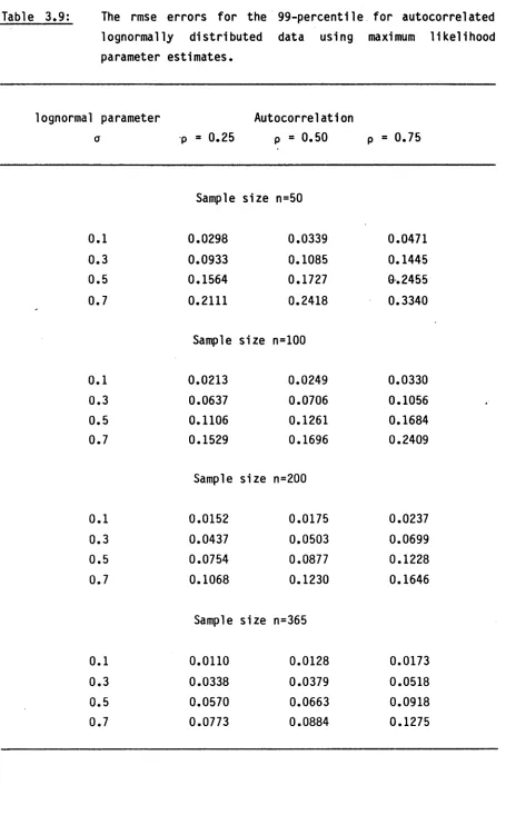
3.3.3 The re la tiv e root mean square errors associated with the estimation of the percentiles of the
lognormal distribution 47
3.3.4 Conclusions for the lognormal distribution 50
3.4 F ittin g the exponential distribu tion to a ir quality data 50
3.4.1 Parameter estimation 51
3.4.2 Monte Carlo simulation studies 51
3.4.3 The re la tiv e root mean square errors associated with the estimation of the percentiles of the
exponential distribution 53
3.4.4 Conclusions for the exponential distribu tion 54
3.5 F ittin g the two-parameter gamma distribution to
a ir quality data 54
3.5.1 Parameter estimation for the gamma distribution 56
3.5.2 Monte Carlo simulation studies 59
3.5.3 The re la tiv e root mean square errors associated with the estimation of the percentiles of the
gamma distribution 60
3.5.4 Conclusions for the gamma distribu tion 63
3.6 F ittin g the two-parameter Weibull distribution to
a ir quality data 63
3.6.1 Parameter estimation 64
3.6.2 Monte Carlo simulation studies 66
3.6.3 The re la tiv e root mean square errors associated
with the estimation of the percentiles of the
Weibull distribution 69
3.6.4 Conclusions for the Weibull distribu tion 70
3.7 Autocorrelation and parameter estimation 70
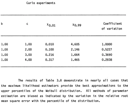
3.8 Conclusions 73
Chapter 4: IDENTIFICATION OF DISTRIBUTIONAL MODELS FOR AIR QUALITY
CONCENTRATIONS
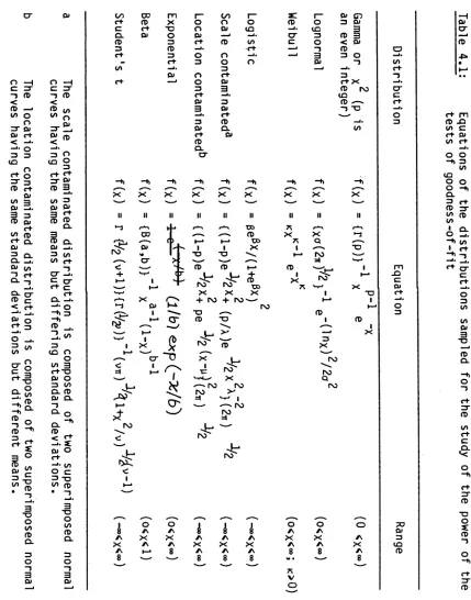
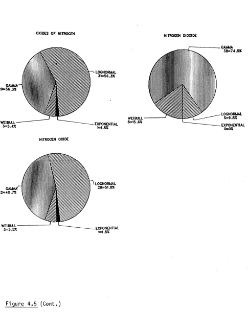
4 .5 Se lec ting a d i s t r i b u t i o n a l model from among
e x p o n e n tia l, gamma, lognormal and Weibull a l t e r n a t i v e s 82
4 . 5 . 1 The s e le c tio n c r i t e r i a 88
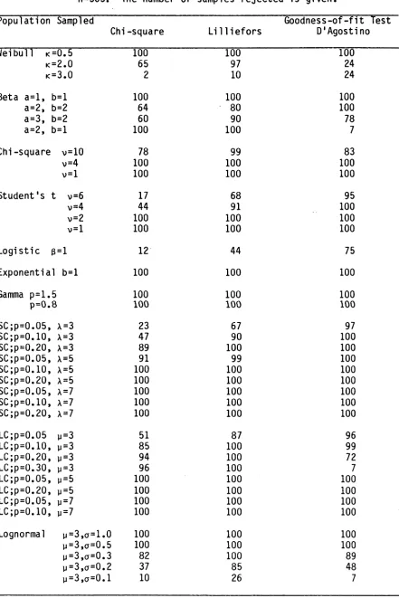
4 . 5 . 2 Simulation procedure and r e s u lts 90
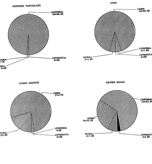
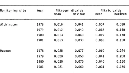
4 . 5 . 3 Model i d e n t i f i c a t i o n procedure 100 4 .6 I d e n t i f i c a t i o n of a d i s t r i b u t i o n a l model f o r a i r
q u a li t y data recorded in Melbourne, A u s tr a lia 101
4 .7 Conclusions 107
Chapter 5: A HYBRID MODEL FOR PREDICTING THE DISTRIBUTION OF AREA SOURCE ACID GAS CONCENTRATIONS
5.1 In tro d u ctio n 108
5.2 The area source hybrid model 109
5 .3 The data set and model assumptions 111
5.4 Estimating the 9 8 - p e r c e n t ile p o llu t a n t concentration 116 5.5 S e n s i t i v i t y of the 9 8 - p e r c e n t ile estim ate to the
K -fa c to r 121
5.6 Discussion 129
5.7 Conclusions 130
Chapter 6: A HYBRID MODEL FOR PREDICTING THE DISTRIBUTION OF POLLUTANTS DISPERSED FROM ROADWAY LINE SOURCES
6.1 In tro d u ctio n 132
6 .2 Line source dispersion models 132
6 .3 Data sets f o r the hybrid model c a l i b r a t i o n 135
6 .4 The GM model 138
6 .5 The Weibull d i s t r i b u t i o n 140
6 .6 Hybrid model c a l i b r a t i o n 142
6.7 Hybrid model v a l i d a t io n 147
6 .8 Discussion 154
C h a p t e r 7: A HYBRID MODEL FOR PREDICTING THE DISTRIBUTION OF SULPHUR
DIOXIDE CONCENTRATIONS OBSERVED NEAR ELEVATED POINT SOURCES
7 . 1 I n t r o d u c t i o n 159
7 . 2 The d a t a s e t 160
7 . 3 D e t e r m i n i s t i c model c omp one nt 164
7 . 4 S t a t i s t i c a l model c o mpone nt 168
7 . 5 Hy b r i d model c a l i b r a t i o n 173
7 . 6 H yb r id model r e s u l t s 177
7 . 7 C o n c l u s i o n s 192
C h a p t e r 8: ASSESSING COMPLIANCE WITH AIR QUALITY CRITERIA USING
STATISTICAL MODELS OF RESTRICTED DATA SETS
8 . 1 I n t r o d u c t i o n 194
8 . 2 The d a t a s e t 196
8 . 3 The e m p i r i c a l q u a n t i l e - q u a n t i l e model 197
8 . 4 K o l mo g o ro v - S mi rn o v t w o - s a m p l e t e s t 199
8 . 5 A p p l i c a t i o n o f t h e m o de l s 200
8 . 6 R e s u l t s and D i s c u s s i o n 201
8 . 7 C o n c l u s i o n s 213
C h a p t e r 9: CONCLUSIONS AND SUMMARY 215
1.1 In tro d u ctio n
The in tro d u c tio n in the United States of the Clean A ir Act Amendments of 1970 and 1977, which included the prevention of s i g n i f i c a n t d e t e r i o r a t i o n , a i r q u a li t y maintenance plans and new source p erm its, i n i t i a t e d a su b s ta n tia l and continuing research e f f o r t in to the development of a i r q u a li t y models in t h a t country. These amendments saw the adoption of an approach to the control of a i r p o llu tio n which defined a i r q u a li t y management as the re g u la tio n of p o llu ta n t emissions in such a manner as to achieve a s p e c ifie d set of national ambient a i r q u a li t y standards or goals (De Nevers et a l . , 1977). This d e f i n i t i o n im p lie s , along with the statement of a i r q u a li t y g oals, th a t estimates of the p o llu ta n t emissions, observations of ambient a i r q u a li t y and models f o r the dispersion of a i r p o l lu t a n t s , be a v a i l a b l e . This a i r q u a li t y management approach to the control of a i r p o llu tio n has been adopted in numerous cou ntries (Campbell and Heath, 1977).
Mathematical models f o r the dispersion of a i r p o llu ta n ts may be constructed f o r s c i e n t i f i c understanding with an aim to exp lain the complex d e t a i l of the physical and chemical processes involved. A l t e r n a t i v e l y models may be developed f o r the purpose of a i r q u a li t y management. While the former approach can in v o lv e considerable complexity of d e s c r ip t io n , the l a t t e r requires only t h a t d e t a i l comensurate with the aims of a i r q u a li t y management and sympathetic to the a v a ila b le a p r i o r i inform ation be incorporated w ith in the model.
The aim of t h is th e s is is to demonstrate t h a t simple but e f f e c t i v e models can be constructed f o r the purpose of a i r q u a li t y management in s p ite of problems associated with poor data and in some cases l im ite d knowledge. The models are used to p r e d ic t ambient p o llu ta n t concentrations in a form th a t allows d i r e c t comparison with a i r q u a li t y c r i t e r i a . The models are simple only in the sense th a t they contain as few parameters as are necessary fo r good p r e d ic t io n . Importantly the models developed y i e l d estimates of the u n c e rta in ty associated with model p r e d ic t io n s . This form of model o u tp u t, while suited to other a p p lic a t io n s , is of p a r t i c u l a r importance to the problem of a i r q u a li t y
1.2 The air pollution problem
The term 'a i r pollution' is defined here to mean the addition of any substance to the atmosphere from sources which directly or through transformation is present at a concentration sufficiently above normal ambient levels to produce a measurable effect upon humans, ecosystem or
materials. A pollutant may be a substance that has been manufactured or
is naturally occurring and may be a gas, aerosol or solid.
Gaseous pollutants added directly to the atmosphere include the
oxides of nitrogen, sulphur and carbon to name but a few. These
pollutants are usually termed primary pollutants whereas the secondary pollutants, including ozone and compounds derived from the sulphur and nitrogen oxides, are produced in the atmosphere by chemical reaction. These chemical reactions can take place between the primary pollutants,
the normal constituents of the atmosphere and other secondary
pollutants. Secondary pollutants are also produced by the decay of
radioactive substances.
Perhaps the most well known form of secondary pollution is
collectively known as photochemical smog. Unlike the primary pollutants
such as sulphur dioxide and particulates which are produced by the combustion of coal, photochemical smog represents a complex series of reactions involving nitrogen oxides, non-methane hydrocarbons and sunlight
(Seinfeld, 1975). Photochemical smog is generally associated with citie s
possessing large motor vehicle populations, poor dispersive conditions such as occur in river valleys and high solar radiation. Los Angeles is probably the best known of the citie s experiencing photochemical smog and was the f i r s t to report a severe episode for which acute eye i r ita tio n and
sore throats were indicators. In Australia the cities of Sydney,
Melbourne and Brisbane experience high levels of photochemical smog (Lawlor, 1982).
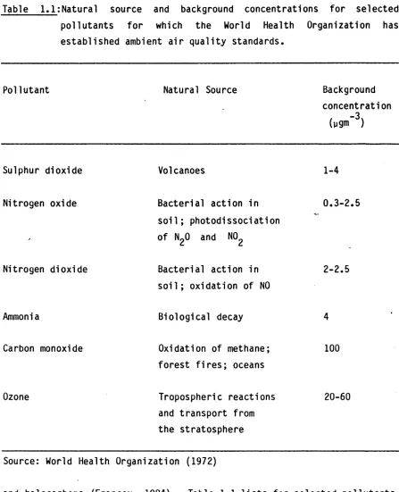
While i t would be desirable to eliminate air pollution
altogether, economic constraints and the presence of natural background
pollutant concentrations makes this task all but impossible. Australia
Table l . l: N a t u r a 1 source and background concentrations f or selected pol 1utants
established
f o r which the World Health ambient a i r q ual i ty standards.
Organization has
Pollutant Natural Source Background
concentration
( u g m “ 3 )
Sulphur dioxide Volcanoes 1-4
Nitrogen oxide Bacterial action in
s o i l ; photodissociation of N^O and NO^
0 . 3 - 2 . 5
Nitrogen dioxide Bacterial action in
s o i 1 ; oxidation of NO
2-2.5
Ammonia Biological decay 4
Carbon monoxide Oxidation of methane;
f orest f i r e s ; oceans
100
Ozone Tropospheric reactions
and transport from the stratosphere
20-60
Source: World Health Organization (1972)
[image:13.541.49.496.78.629.2]Air pollution affects the well-being of humans, ecosystems and materials over areas ranging in scale from the local through regional and national and, more recently, to the global scale. With the advent of the
Industrial Revolution the effects of air pollution were no longer
restricted to the area local to the pollution source. The long range
transport of acid gases in Europe and North America (United States National Research Council, 1983a) is not only due to the increased emission levels of recent times, but is also due to the construction of
t a l l chimneys from which the primary pollutants are emitted. This
strategy has converted a local pollution problem to one of international concern requiring international cooperation to ameliorate.
Examples of air pollution problems of global concern include the effects of the halocarbons upon the ozone layer (United States National Research Council, 1976) and the potential effects of increasing carbon dioxide levels (Bach, 1978; United States National Research Council,
1983b). It is hypothesised that the increased carbon dioxide levels
brought about by the burning of wood and fossil fuels will lead to a
global increase in temperature. Some of the effects of this increase in
temperature are considered to be raised sea levels flooding many of the world's c i t i e s , and changes in the pattern of rainfall significantly altering agricultural production (United States National Research Council; 1983b).'
In this thesis the problems examined have been restricted to the regional and local scales. Models are developed for area sources such as c i t i e s , and for large point sources which affect the air quality over
large regions. At the local scale a model is developed to describe the
dispersion of pollutants from roadway line sources. Obviously this model
could be applied many times to represent a regional road network although this problem is not considered in this thesis.
In summary, air pollution arises from interactions within a complex system involving the emission of numerous pollutants from a wide
range of sources. These pollutants are dispersed within the atmosphere
where they may undergo transformation. Ultimately they affect ecosystems
1.3 Modelling atmospheric dispersion - a badly defined system
In a study of the long-range transport and deposition of pollutants Venkatram and Pleim (1985) considered that our understanding of th is system is derived from two modelling approaches, namely the th e o re tic a l or 're d u c tio n is t' method and the empirical or ' h o l i s t i c ' method. This is true not only for long range transport of po llu tan ts but for the study of atmospheric dispersion in general (Hanna, 1982a). Venkatram and Pleim (1985) consider that empirical models are important because of the d i f f i c u l t y in developing th e o r e t ic a lly based models due to gaps in our understanding of the components of these models, lack of the extensive data sets required to run such models, and that these models generate responses which are not readily i n t e l l i g i b l e . They considered that empirical models whose structure is closely tie d to observations were required to complement th e o re tic a l models.
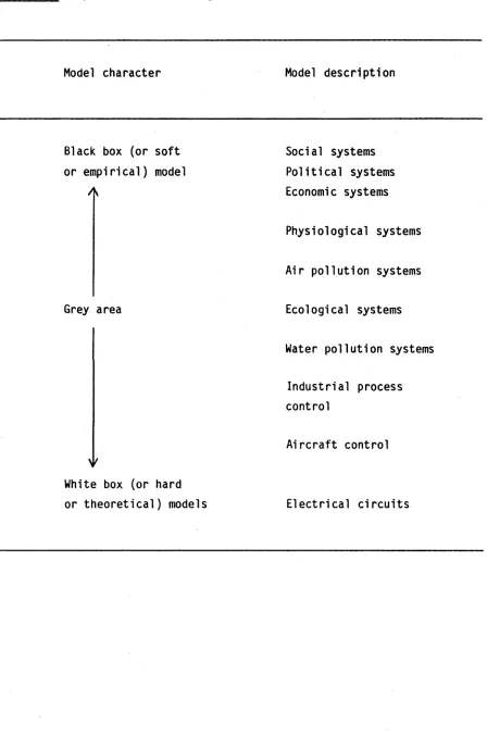
While Venkatram and Pleim (1985) perceive modelling approaches at two extremes, they c it e the work of Beck (1981) who describes the development of mathematical models as occurring over a wide spectrum. This spectrum varies from 'hard' systems such as e le c t r i c a l systems, to 's o f t ' systems such as social systems. The degree to which the behaviour of the system may be in ferred a p rio ri and planned experiments undertaken to v e rify the model formulation determines the 'hardness* of the system. Karplus (1976) and Vemuri (1978) describe th is spectrum of models as ranging from white box systems (hard) to black box systems ( s o f t ) . Air po llu tio n systems are considered to f a l l w ithin the grey area between these two extremes. Table 1.2 l i s t s examples of systems lying w ith in th is spectrum.
Beck (1981) cites the work of Young (1978) who has suggested that natural environmental systems are d i f f i c u l t to analyse in mathematical terms because t h e i r underlying mechanisms tend to be 'badly d e fin e d '. The poor d e f in it io n arises from the i n a b i l i t y to conduct planned experiments on the system. Thus models lying w ithin the grey area, as delineated in Table 1.2, may not necessarily move inexorably towards a white box model where a near complete understanding of the system has been reached. Hence uncertainty may remain a s ig n ific a n t
Table 1 . 2 : Spectrum of modelling a c t i v i t i e s .
Model character Model description
Black box (or soft or e m p iric a l) model
A
Grey area
White box (or hard or t h e o r e tic a l) models
Social systems P o l it ic a l systems Economic systems
Physiological systems
Air p o llu tio n systems
Ecological systems
Water p o llu tio n systems
In dustrial process control
A ir c r a f t control
[image:16.541.51.499.94.782.2]Faced with badly defined environmental systems Young (1978, 19&1, 1982]} developed a methodology fo r the systematic analysis of systems based upon several considerations. While the methodology was s p e c ific a lly developed fo r dynamic systems some of the concepts are also relevant to systems that are modelled as s t a t i c . These concepts are:
( i ) while the system is nominally complex i t s passively observed behaviour is often dominated by r e l a t i v e l y simple lin e a r or nonlinear relatio n sh ip s;
( i i ) that hypothetico-deductive procedures of the s c i e n t i f i c method be used to establish those modes of behaviour consistent with the observations; and
( i i i ) the id e n t i f i a b l e modes of behaviour may not provide a t o ta l description of the system as fu rth e r data c o lle c tio n may suggest that other modes are also s ig n if ic a n t .
This approach to modelling environmental systems has been
iq?2A
applied successfully to water q u a lity problems by Young (T381) , Hornberger and Spear (1980) and Jakeman et a l . (1984) and has been applied to the study of a i r q u a lity by Steele (1981) and Steele and Jakeman (1980). Most of these studies applied recursive methods of time series analysis
e-K— ( 1980) I Jakeman et a l . (1980), and Jakeman and iuuny 1983).
In th is study, while time series analysis methods have not been employed as the a n a ly tic t o o l , the general p rin ciples of modelling badly defined systems as outlined above have been adopted. Thus models developed here are simple models aimed at producing a parametrical ly e f f i c i e n t description of the a i r q u ality data. The models developed are not black box models but are simple descriptions of the physical dispersive system where many of the state variables and mechanisms are capable of c le a r in t e r p r e t a t io n .
1.4 Thesis o u tlin e b
developed by Young (1974, 1976), Young and Jakeman
the development of the air quality models. In Chapters 3 and 4 the methods of parameter estimation and model identification necessary for the improved use of s t a t i s t i c a l models and for the development of s ta t i s t i c a l
model components of hybrid models are examined. The subsequent three
chapters form a series of investigations into the modelling of air
quality. To demonstrate the generality of the approach models are
constructed for the three key emission source regimes, namely for area,
line and point sources. The problem of designing monitoring networks to
provide maximum information return in terms of assessing compliance with
air quality standards is considered in Chapter 8. A more detailed
description of the individual chapters follows.
In Chapter 2 models capable of describing the distribution of
pollutant concentration are examined. The two major approaches,
deterministic and s t a t i s t i c a l modelling, and the advantages and
limitations of each are considered. The combination of these two
modelling approaches, the hybrid modelling methodology, is described here.
Numerous methods are availible for estimating the parameters of distributional models considered applicable to the study of air quality
data. Chapter 3 examines various methods of parameter estimation using
Monte Carlo experimentation. For each of the methods the bias, variance
and more practical considerations such as the computational demands of the
methods are examined. A method for generating approximate confidence
intervals at percentiles of interest for each of the distributional models examined in the Monte Carlo studies is presented.
In Chapter 4, employing the methods of parameter estimation examined in Chapter 3, model identification procedures are considered. Based upon an examination of their performance a new procedure for the selection of appropriate distributional models for air quality data is
presented. The model identification procedure is applied to air quality
observations recorded in Melbourne, Australia.
The problem of predicting the dispersion of pollutants from roadway line sources is considered in Chapter 6. A b rief review of models applied to roadway line sources and th e ir performance is given. On the basis of model calibration and model validation exercises the hybrid model is found to yield considerably improved estimates, when compared with the
deterministic model applied alone, of the upper percentiles of the
distribution of pollutant concentrations.
Chapter 7 describes the development of a hybrid model for the dispersion of sulphur dioxide from point sources. The calibration of the
deterministic component of the hybrid model is performed using the
percentiles rather than time-wise matched pairs. The hybrid model
produces estimates of pollutant concentration at 24-h, 8-h, 3-h, 1-h and
0.5-h averaging times. Compared with the deterministic model applied
alone the hybrid modelling approach provides a significant improvement in
the prediction of the upper percentiles of the distribution of pollutant
concentrations observed about point sources. Approximate confidence
intervals were derived for model estimates and were found to provide reasonable bounds for model uncertainty.
The need to design a ir quality monitoring networks to obtain the
maximum return of information forms the basis of the work reported in Chapter 8. Here three approaches for increasing the spatial resolution
of a ir monitoring networks based upon restricted data sets are
considered. The importance of the application of a model id e n tifica tio n procedure such as that developed in Chapter 4 is demonstrated. Where a second complete data set is available, an empirical quantile-quantile
model may be applied. This modelling approach does not require the
assumption of a distributional form for the a ir quality data. The
empirical quantile-quantile model is found to provide the best estimates of the upper percentiles of the pollutant d is trib u tio n .
F in a lly , in Chapter 9 a summary of the principal conclusions of
the thesis and a discussion of future directions that this research may
2 . 1 I n t r o d u c t i o n
This c ha pt e r examines t h e two major approaches t o t he problem of mode ll in g t h e d i s t r i b u t i o n o f a i r p o l l u t a n t c o n c e n t r a t i o n s . I t should be noted t h a t t h i s t h e s i s i s concerned w it h p o l l u t a n t s which may be consi dered i n e r t , or a t l e a s t r e l a t i v e l y i n e r t , over t he measurement t i me s c a l e . The two m od e ll in g approaches consi dered can be broadl y c l a s s i f i e d as d e t e r m i n i s t i c and s t a t i s t i c a l m o d e l l i n g . Here t h e term ' d e t e r m i n i s t i c ' r e f e r s t o models f o r mu l at ed using p hysi cal l aws. These models y i e l d a mech a ni st i c d e s c r i p t i o n of t h e d i s p e r s i o n o f p o l l u t a n t s w i t h i n t h e atmosphere.
The o r i g i n s of t h e d e t e r m i n i s t i c approach t o model li ng d i s p e r s i o n are a t t r i b u t e d t o t he work o f T a y l o r ( 1 9 15 , 1921, 1927) who measured t u r b u l e n t v e l o c i t i e s i n t he h o r i z o n t a l plane using t h e widths of t he t r a c e s produced by t he wind speed and d i r e c t i o n . This work was f o l l o w e d by f u l l s c a l e t r a c e r experiments performed by Sutton ( 1 932 ,
1 9 3 4) . Under near i d e a l c o n d i t i o n s t he f i r s t s p e c i f i c a t i o n s o f t he cross wind and v e r t i c a l spread of suspended m a t e r i a l were obt ai ne d over a range of a few hundred metres from t h e source.
application of d is tr ib u tio n a l models to a i r q u a lity data. Attempts have been made to in f e r a p r io ri the d is trib u tio n that a i r q u ality data should fo llo w . However, to date th is approach has met with only lim ited success.
A second type of s t a t i s t i c a l modelling undertaken in th is thesis relates the percentiles of the d is trib u tio n of p o llu tan t concentration using a simple lin e a r re la tio n s h ip . This model, termed an empirical q u a n tile -q u a n tile model (Chambers et a l . , 1983), is of importance to the design of monitoring networks and the development of monitoring strategies where re s tric te d data sets are c o lle cte d .
In th is chapter the d eterm inistic and s t a t i s t i c a l modelling approaches w i l l be examined with the view to id e n tify in g the strengths and the lim ita tio n s of each in determining the d is tr ib u tio n of pollutant observations. Further, the concept w i l l be introduced that these two modelling approaches can be combined in such a manner so that the strengths of each approach are exploited while the weaknesses of each are attenuated.
2.2 Deterministic a i r q u a lity models
In th is section determ inistic models fo r the dispersion of in e rt gases within the atmospheric boundary layer are c r i t i c a l l y examined. There are many reviews which cover the f u l l range of a i r q u ality models including those by Lamb and Seinfeld (1973), Eschenroeder (1975), Johnson et a l . (1976), Turner (1979), Simpson and Hanna (1981), Hanna (1982a) and Geraghty and Ricci (1984). The various theories of atmospheric dispersion are examined on the basis of how each predicts p o llu tan t concentrations. Thus i t is the d if fe r e n t model treatments of turbulent d iffu sio n which w i l l be examined here. An understanding of the accuracy of a i r pollution model predictions is important in environmental management as th is allows an assessment of the risk of exceeding a i r q u a lity standards to be
undertaken. Accordingly a discussion of the accuracy with which
2.2.1 Gradient transport model
The set of equations that form the basis for the development of mathematical models for the dispersion of pollutants within the planetary
boundary layer describe the motions of a viscous, compressible, Newtonian f lu id in a rotating system. The equation of continuity, which is an
expression of the conservation of mass is stated as
p + iHp +
+ I * . . o
a t ax ay az
(2.1)
where p is the instantaneous density and u, v, w are the instantaneous
velocity components describing the motion of the flu id in the x, y and z
directions respectively, at the point (x ,y ,z ) at time t and in a Cartesian co-ordinate system. Equation (2.1) may also be written in the form
au av aw - l dp
— + — + — = ---c_
ax ay az p dt
(2.2)
where the individual terms on the l e f t side are usually at least two
orders of magnitude larger than the right side. Consequently the
assumption
au t av | aw
ax ay az
0 (2.3)
that the atmosphere is incompressible is a good and useful approximation (e.g. see Businger, 1982).
The d iffe r e n tia l equation which has become the starting point of
most mathematical treatments of diffusion from sources is a generalization of the classical equation for the conduction of heat in a solid and is
essentially a statement of the conservation of the mass of suspended material (Pasquill and Smith, 1983). Denoting the concentration by x units of mass per unit volume of a flu id which is assumed incompressible
IX. = _ [ Mu x) + 3 ( vx ) + 3( wx ) i (2.4)
a t ax ay az
The above equation constitutes only one of five coupled fundamental equations describing all aspects of the interaction of chemically active constituents in a fluid (Businger, 1982). However, since air pollutant concentrations only rarely exceed a few parts per million (ppm) by volume, the presence of air pollutants will produce insignificant changes to the heat balance of the atmosphere. An exception to this rule is the reduction in solar radiation intensity resulting from air pollutants over urban areas (Bach, 1971). In general, the assumption that meteorology remains unchanged i s reasonable. This assumption allows equation (2.4) to be solved with the fluid v e lo c it i e s u, v, w considered independent of the concentration terms x-j •
Unfortunately the complexity of turbulent flow is so formidable that even i f we were able to describe i t s structure in d e t a i l , comprehension would be close to impossible (Businger, 1982; Pasquill and Smith, 1983). This has led to the development of the description of turbulent flow in terms of i t s s t a t i s t i c a l chara cter ist ics . It has been assumed therefore that the fluid motions can be separated into a slowly varying mean flow (ü,v,w) and a rapidly varying turbulent flow (u, , v , ,w'). Hence the instantaneous velocity components in a rectangular co-ordinate system are given by
u = u + u
v = v + v (2.5)
I
w = w + w
Similarly the instantaneous concentration terms x.j are themselves random variables
+
I
Writing u, v, w and x as the sum of a mean and eddy fluctuations as given in equations (2.5) and ( 2 .6 ) , expanding, averaging and rearranging equation (2.4) gives
i i + j i i + v l i + w i i
- [
8
(-u.Y .) + i^x.' + aK x1.)]
( 2 . 7 )a t ax ay az ax ay az
Physically the velocity components refer to an element of a ir
passing through a specified point. In the Eulerian-space system the
velocities are in principle specified at a ll positions in the fie ld of flow at a given instant. In the system known as Lagrangian, the concern
is with the variations in time of the velocity of a particular element, which is of course continuously changing its position. The analysis of
atmospheric turbulence is usually concerned with the fluctuation recorded by a fixed instrument responding more or less rapidly to the relative
motion of the a i r . This situation is customarily regarded as equivalent
to the Eulerian-space description (Pasquill and Smith, 1983), the
equivalence is based upon the hypothesis that the sequence of variations at a fixed point is s t a t i s t i c a l l y the same as the instantaneous spatial variation.
The gradient-transport approach assumes that turbulence causes a
net movement of material down the gradient at a rate which is proportional to the magnitude of the gradient. The turbulent transfer of material in this manner is referred to as a simple diffusion process (Pasquill and Smith, 1983). By replacing the eddy flux terms by the simplest gradient-transport forms equation (2.7) becomes
d r = - L (Kx H .) + _L (K &-) + - 1 (K lx-) (2 .8)
dt ax x ax ay y ay az az
This equation allows for differences in the eddy
independent of x, y or z then the resu ltin g equation and type of d iffu sio n implied are Fickian. In th is case the d is tr ib u tio n of material is of a Gaussian form with variances
a 2 = 2K t = 2K x/u
x x x (2 .9 )
however, experimental studies have shown th a t the equivalent values of K vary systematically with the time of t r a v e l , with the p o s itio n , and with the scale of the d iffu s io n process (Pasquill and Smith, 1983).
The gradient-transport formulation may be expected to be the most successful when the d iffu s iv e action of the turbulence is e f f e c t i v e ly confined to scales small r e la t iv e to the volume occupied by the suspended m a te ria l. For v e rtic a l spread th is condition is approached for ground level releases of p o llu ta n ts . However, i t is not met in the case of tim e-mean la te r a l dispersion from a continuous point source and for v e rtica l dispersion from an elevated source.
2 .2 .2 Gaussian plume models
The Gaussian plume model is the most widely applied d iffu sion model (Hanna, 1982a; Turner, 1979). The Gaussian plume model takes i t s name from the assumed Gaussian form describing the v e rtic a l and cross-wind concentration p r o f i l e s . As noted e a r l i e r the Gaussian plume formula can be derived from equation (2 .8 ) providing that the turbulence is homogeneous and stationary and only a point source is considered. The Gaussian expression is (e .g . Hanna, 1982a)
2 2 2
x ( x , y , z ) = — 9— exp ( ^ —) [exp ( ~^Z~H^ ) + exp ( ~^Z+H^ )] (2.10)
2nUo o 2 2 2 2
y z z
The application of equation (2.10) is based upon the following assumptions that:
(a) both the emission rates and meteorological
conditions have attained a steady s ta te ;
(b) a constant windspeed and wind direction, valid for the entire region, may be specified;
(c) no absorption or generation by the ground occurs;
(d) there is no inversion layer;
(e) the diffusiv ities in the vertical and cross-wind directions vary only with downwind distance and are constant in the diffusion domain; and,
(f) the pollutant does not undergo chemical reaction.
Observations of passive plumes have confirmed that the Gaussian form is a satisfactory description for the cross-wind distribution, at least for
ensemble averages (Pasquill and Smith, 1983). In spite of the above
simplifying assumptions necessary for the application of the Gaussian plume model, this model has seen widespread application (Simpson and
Hanna, 1981; Turner, 1979). This model, in various forms for point area
and line sources constitutes the basis of the UNAMAP (User's J^etwork for Applied Modeling of Air pollution) developed by the United States Environmental Protection Agency as an aid to the development of air quality management strategies.
The Gaussian plume model has also been modified by Davis and Metz (1978) for the special case of particulate matter to allow for
surface deposition and reflection. More recently Hanna et a l . (1984)
modified the Gaussian plume model for application in complex te rrain . The Gaussian plume formula as stated in equation (2.10), with suitable integration may be applied to line and area sources. The specific details of the Gaussian plume models developed in this study for line and point sources are presented in Chapters 6 and 7. The models developed in these chapters employ the most recent improvements to the Gaussian plume model
improvements is limited only by the availability of the data necessary for their implementation.
(see Hanna in such areas as wind speed evaluation, plume rise
2 . 2 . 3 Rollback models
The ro llb a c k model was developed to provide a simple method by which source p o llu ta n t emissions could be assessed (Chang and Weinstock,
197 5 ). The o r ig in a l model assumes t h a t p o llu ta n t concentrations are d i r e c t l y p ropo rtional to emissions according to some simple r e l a t i o n s h i p . Thus the emission control requirements are presumed p ro p o rtio n a l to the amount by which the peak p o llu ta n t concentration exceeds the standards. The n o n lin e a r it y of the atmospheric processes l i m i t s the usefulness of the ro llb a c k model to a ro le in which a f i r s t rough estim ate is made of the emission con trols re q u ire d . The sim plest form is of the type
X = ke + b (2 .1 1 )
where x is The p o llu ta n t concentration due to emissions at a ra te e , with b being a measure of the background p o llu ta n t concentration and k the constant o f p r o p o r t i o n a l i t y . All the e f f e c t s associated with the meteorology, the d i s t r i b u t i o n of sources and a l l other fa c to rs are included in k. De Nevers and Morris (1975) d e fin e k in terms of the highest concentration
k (xmax - b)/e ( 2. 12)
where x max is The highest p o llu ta n t concentration in the region of i n t e r e s t . The allo w ab le emission ra te e is then
max
e max
e (* s t d
xmax
( 2 .1 3 )
where x st.d is The a i r q u a li t y standard required f o r the p o llu ta n t being considered.
Xi E k . . e . + b
i j J (2.14)
where is the concentration at receptor i , ej is the emission rate at source j , and is the source-receptor in te ra c tio n fo r source j and receptor i . Peterson and Moyers (1980) have extended the above model to the case where continuous measurement of ambient concentrations and emissions are av aila b le and recorded over time in te rv a ls corresponding to a i r q u a lity standards.
Georgopoulos and Seinfeld (1982) examined these rollback
calculatio ns and recommended the replacement of x and x . with the
r Amax Astd
expected mean values, denoted E(x ) and E(x . ,) respectively where E(xstd ) represents the expected mean concentration from a d is tr ib u tio n in which x stcj is an extreme. Applying the expected values in rollback calcu latio n s allows fo r the conservation of mass of non-reactive p o llu ta n t. Georgopoulos and Seinfeld (1982) then considered whether the concentration x would increase lin e a r ly with emissions as does the expected value E(xmax) . They found that l i n e a r i t y holds fo r the p a r t ic u la r case where po llu tan t concentration is lognormally d istrib u te d and meteorological conditions remain unchanged. In p a r tic u la r the geometric standard deviation must remain unchanged. There is of course ample evidence in dicatin g that these conditions are ra re ly met (Simpson et a l , 1985). Thus rollback models are only useful at the i n i t i a l stages or as screening models with which a crude in d ication of future trends may be determined.
2 .2 .4 Box models
A useful evaluation of the e ffec ts of a large area source may be made using the simple box model described by Gifford and Hanna (1971,
1973), referred to as the ATDL (Atmospheric Turbulence and Diffusion
Laboratory) model. This model has seen widespread application
(Eschenroeder, 1975; Pasquill and Smith, 1983). The ATDL model is applicable to urban area sources in which the emissions are assumed uniform over grid squares that may vary in size from 1- to 10-km square. For a grid pattern with uniform source strengths in each square, the
1-b -1
(2/i r) (ax/ 2 ) [ua (1- b) ]
.{Qn + I Qi (21 + l ) 1_b - {21 - l ) 1_b}
0 i =1 1
(2.15)
where N is the number of upstream grid squares contributing to the concentration in the grid square under consideration (designated by the subscript o), a and b are parameters dependent on atmospheric s t a b i l i t y ,
ax is the size of the grid square, u is the average horizontal windspeed assumed to be in the x-direction, and Q (i = 0 , 1, 2, . . . , N) are the area source strengths for each grid square.
When the spatial variation in the source strengths are smooth slowly varying functions the above equation may be simplified (Hanna,
1971) to
(2.16)
where C is a constant that depends on atmospheric s t a b i l i t y . Equation (2.16) follows from (2.15), only for smooth area source distributions in
which the terms involving Q.. (i * o) in (2.15) are significantly less
than the Qq term. Benarie (1976) has shown that this equation is widely applicable.
The ATDL model has been shown to yield predictions that compare favourably with those given by four more complex models (Hanna, 1971) and has been demonstrated to be applicable to a wide range of urban environments including Frankfurt (Hanna and Gifford, 1977), Canberra (Daly and Steele, 1976) and Milan (Gualdi and Tebaldi, 1982).
X - CQuP ( 2 . 17 )
where p i s t h e windspeed exponent which may vary between 0 and - 1 . B en a r i e c o n s i d e r e d t h a t only where a d v e c t i v e mixing dominates would t h e -1 power, as s t a t e d i n e q u a t i o n ( 2 . 1 6 ) , be c o r r e c t . In t h e c a s e of pre do mi na nt c o n v e c t i v e mi xi ng , Bena ri e s t a t e s t h a t a d v e c t i o n would n o t change t h e c o n c e n t r a t i o n and t h u s windspeed shoul d have an exponent of z e r o . B en a ri e found from a review of e x p e r im en t al s t u d i e s t h a t t h e v a l u e o f t h e exponent ranged between - 0 . 2 and - 0 . 5 . Bena ri e a l s o s p e c u l a t e d t h a t t h e exponent p may be a c l i m a t o l o g i c a l c h a r a c t e r i s t i c f o r any gi ve n c i t y and may vary with s e a s o n .
Daly and S t e e l e (1976) and Simpson e t a l . (1983) have r e l a x e d t h e a ss umpt io n i mp l i ed in e q u a t i o n ( 2 . 1 6 ) t h a t t h e windspeed and p o l l u t a n t c o n c e n t r a t i o n a r e i n v e r s e l y r e l a t e d as matched p a i r s of o b s e r v a t i o n s . I n s t e a d i t i s assumed t h a t o p p o s i t e p e r c e n t i l e v a l u es of windspeed and a i r p o l l u t i o n d i s t r i b u t i o n s a r e r e l a t e d by a simple i n v e r s e r e l a t i o n s h i p , s t a t e d as (Simpson e t a l . , 1983)
xP K
u 100-p
( 2 . 18 )
where Xp i s t h e a i r p o l l u t i o n c o n c e n t r a t i o n c o r r e s p o n d i n g t o t h e p- p e r c e n t i l e o r d i n a t e of t h e a i r p o l l u t i o n c u m u l a t i v e f r e qu e nc y d i s t r i b u t i o n , u ^ i s t h e windspeed c o r r e s p o n d i n g t o t h e ( 1 0 0 - p ) - p e r c e n t i l e o r d i n a t e of t h e windspeed c u mu la t iv e fr eq ue n cy d i s t r i b u t i o n and K i s a c o n s t a n t . The c o n s t a n t i s d e r i v e d from t h e r e l a t i o n s h i p between x and u , ™ f o r each sampling s t a t i o n under c o n s i d e r a t i o n over some p e r c e n t i l e range f o r which K i s a p p r ox i ma t e l y c o n s t a n t . Simpson e t a l .
(1983) use t h e medians t o e s t i m a t e K so t h a t
K
Knox and Lange (1974) and Benarie (1976) suggested a s im ila r measure and noted that the constant K derived in th is manner requires no d ire c t knowledge of the source strength. Simpson et a l . (1985) observed for to ta l suspended p a rtic u la te s and acid gas observations that xpuiQ0 p is reasonably constant over the 30-70 p e rc en tile range. Thus fo r t h e i r data at least th at- the model given by equation (2.18) is a good representation of the relatio n sh ip of the s t a t i s t i c a l d is trib u tio n s of windspeed and p o llu tan t concentration fo r at least the 30-70 p ercen tile
range.
The model as given in equation (2.18) was combined with the assumption of a lognormal d is tr ib u tio n of p o llu ta n t concentrations and windspeed data to y ie ld estimates of the e n tire d is tr ib u tio n of p o llu tan t concentration (Simpson et a l . , 1983). The p -p e rc e n tile concentration is easily found from
x
P (2.20)
where ß^ is the geometric standard d e v ia tio n , the geometric mean (median) of the windspeed data and z is the standard v a ria te
P
corresponding to the p -p e rc e n tile . This model, equation (2.20) with ( 2 .1 9 ) , has been applied by Simpson and Jakeman (1985) to forecast worst case po llu tio n scenarios fo r acid gas and suspended p a rtic u la te s due to urban in d u s tria l development. T h irty years of windspeed data were parameterised to obtain estimates of au and ß^ fo r each year in order to obtain a range of extreme values in (2 .2 0 ) fo r a given K.
2 .2 .5 Deterministic model performance
Several discussions have recently appeared on the accuracy a ttain a b le in the prediction of a i r p o llu tio n concentrations (Hanna,
1982a; Benarie, 1976, 1982; Pasquill and Smith, 1983; Venkatram,
set of unresolved residual turbulent flows. Therefore the best an air quality model can be expected to produce are estimates of average
concentrations (Venkatram, 1983) and a model estimate can be expected to
diffe r from the corresponding observation.
This conclusion is supported by the study of Hanna (1982c) who from an analysis of a* meteorological and pollutant data sets examined the effect of “natural variability ". Hanna considered the variation inherent
in pollution concentrations based upon the division of pollutant
observations into 18 wind direction classes, 10 wind speed classes and 7
s t a b ili ty classes. The data examined were hourly carbon monoxide and
sulphur dioxide data recorded at 25 stations in St Louis for all hours of
1976. Hanna (1982c) concluded that the natural variability of hourly
average concentrations in St Louis for given meteorological and source conditions is typically a factor of two.
It could be argued that the limitations encountered in the application of deterministic models are due to the lack of meteorological information, particularly in respect of special factors which are required for the full application of the more complex models. However, i t has been recognized that the cost of the required observational programmes would more than likely outweigh any benefits achieved from the increased r e l i a b i l i t y of pollutant concentration estimates (Pasquill and Smith,
1983). The proposal for increased data collection has been further
criticized on the basis that the underlying dispersion relations apply at best only to idealized situations of air flow and topography which are rarely of practical significance particularly when determining the more
adverse conditions of dispersion (Benarie, 1982; Pasquill and Smith,
1983).
It is not surprising then, that comparisons of simple and complex modelling methodologies have shown that model performances are similar (Simpson and Hanna, 1981; Benarie, 1976, 1982). Pierce (1984) in a study of point source Gaussian plume models used to estimate hourly sulphur dioxide concentrations, noted that the more sophisticated models
did not appreciably outperform the routinely applied models. Given the
greater input data requirements and the usually significantly larger computational requirements of the more complex models, a simple model is
demands of a model for hourly pollutant observations recorded over two
years limited the complexity of the model that could be developed. The
models developed in this thesis are based upon the Gaussian plume
assumption which allows an analytical approach. On the other hand, the K
diffusion models require numerical solution employing methods such as f i n i t e elements or f i n i t e differences which themselves may introduce error
(Chock, 1985a; Pasquill and Smith, 1983).
For most practical applications the accuracy of air quality models for ensemble averages is not expected to be less than several tens percent, while for comparisons with individual observations factors of two or more may be expected (Benarie, 1976, 1982; Hanna, 1982b; Pasquill and
Smith, 1983; Simpson and Hanna, 1981). For the point source Gaussian
plume model Nieuwstadt (1980) found that an accuracy of a factor of 2 for mean concentrations, and for the upper percentiles a factor 4, could be
expected. Turner and Irwin (1982) when using a point source Gaussian
plume model to predict the second highest 3-h and 24-h average sulphur
dioxide concentrations observed considerable scatter between model
predictions and observations. For the 37 data sets they examined for 24-h periods 68% of model predictions were within a factor of 2 while for 3-h
periods 84% were within a factor of 2. No significant biases in model
estimates were revealed. Venkatram (1984) in a theoretical analysis of
the uncertainty of model predictions of 1-h average concentrations
considered that 25% of the observations would lie outside a factor of two of the maximum predicted concentration.
In summary the level of uncertainty expected from simple
deterministic models would be in the order of a factor of 2 for ensemble
means and larger for the more extreme pollutant concentrations. Finally
Pasquill and Smith (1983) note th a t, "It remains to be seen whether any significant improvement in this capability will ensue as a consequence either of the ever-increasing sophistication in the studies of atmospheric
flow or of the continuing elaboration in mathematical modelling
techniques“. This view is supported by the theoretical considerations