Statistical analysis of electron lifetimes at GEO: Comparisons with chorus-driven losses

RESEARCH ARTICLE

Key Points:

• Electron lifetimes increase with energy

• Statistical results show good agreement with an analytical model • Above 500 keV, electron lifetimes

increase by a smaller amount

Correspondence to:

R. J. Boynton,

r.boynton@sheffield.ac.uk

Citation:

Boynton, R. J., M. A. Balikhin, and D. Mourenas (2014), Statistical analysis of electron lifetimes at GEO: Comparisons with chorus-driven losses,J. Geophys. Res. Space Physics,119, 6356–6366, doi:10.1002/2014JA019920.

Received 27 FEB 2014 Accepted 24 JUL 2014

Accepted article online 29 JUL 2014 Published online 21 AUG 2014

This is an open access article under the terms of the Creative Commons Attribution License, which permits use, distribution and reproduction in any medium, provided the original work is properly cited.

Statistical analysis of electron lifetimes at GEO: Comparisons

with chorus-driven losses

R. J. Boynton1_{, M. A. Balikhin}1_{, and D. Mourenas}2

1_{Department of Automatic Control and Systems Engineering, University of Sheffield, Sheffield, UK,}2_{CEA, DAM, DIF,}

Arpajon, France

Abstract

magnetosphere is exposed to high-speed streams of solar wind, coronal mass ejections, magnetic clouds, or other disturbances. After this increase, the number of electrons decays back to approximately the initial population. This study statistically analyzes the lifetimes of the electron at Geostationary Earth Orbit (GEO) from Los Alamos National Laboratory electron flux data. The decay rate of the electron fluxes are calculated for 14 energies ranging from 24 keV to 3.5 MeV to identify a relationship between the lifetime and energy of the electrons. The statistical data show that electron lifetimes increase with energy. Also, the statistical results show a good agreement up to∼1 MeV with an analytical model of lifetimes, where electron losses are caused by their resonant interaction with oblique chorus waves, using average wave intensities obtained from Cluster statistics. However, above 500 keV, the measured lifetimes increase with energy becomes less steep, almost stopping. This could partly stem from the difficultly of identifying lifetimes larger than 10 days, for high energy, with the methods and instruments of the present study at GEO. It could also result from the departure of the actual geomagnetic field from a dipolar shape, since a compressed field on the dayside should preferentially increase chorus-induced losses at high energies. However, during nearly quiet geomagnetic conditions corresponding to lifetime measurement periods, it is more probably an indication that outward radial diffusion imposes some kind of upper limit on lifetimes of high-energy electrons near geostationary orbit.

1. Introduction

The fluxes of energetic electrons in Earth’s outer radiation belt strongly vary with geomagnetic activity [Reeves et al., 2003]. Determining the main actors in the energization and loss processes of electrons is essential for providing accurate space weather forecasts of these energetic particle populations, which can damage satellite electronic components [Horne et al., 2013]. Various loss processes are present in the outer belt, such as gyroresonant scattering by whistler mode waves and electromagnetic ion cyclotron (EMIC) waves (e.g., see the review byThorne[2010]), while radial diffusion by electric and magnetic ULF fluctuations can either accelerate electrons or scatter them outward to the magnetopause [e.g., seeShprits et al., 2008; Turner et al., 2014].

Figure 1.(a–g) Figure 5 fromBoynton et al.[2013b] redrawn, which displays a solar wind velocity, density, and pressure; three energies of the logarithmic electron fluxes; and magnetopause position.

Synchronous Orbit Particle Analyzer (SOPA) [Belian et al., 1992], and the 1.8–3.5 MeV electrons are from the Energetic Sensor for Particles (ESP) [Meier et al., 1996].

In Figure 1d, the 1.8–3.5 MeV electron flux increases from 10 to 12 November then remains approximately constant until 18 November, where there is a dramatic loss (a dropout) of high-energy electrons, which coin-cided with a relatively large increase in density. The dropout may be due to strongly enhanced outward transport toward a much closer magnetopause in the presence of an increased dynamic pressure of the solar wind, as observed in recent studies during more disturbed periods [Turner et al., 2013]. It can be seen from Figure 1f that the 270 keV electrons start to decrease immediately after it has peaked and does not plateau like the higher-energy electrons. Instead, the 270 keV electrons decay back to the preevent levels by 17 November. Therefore, the dropout on 18 November, which has a powerful effect on the 1.8–3.5 MeV electrons and a moderate effect on 625 keV electrons, does not influence the 270 keV electrons because on 18 November, the latter fluxes are already relatively low. Thus,Boynton et al.[2013b] hypothesized that the lower energy fluxes most often decay back to preevent levels before any subsequent increase of solar wind density, preventing any marked influence of density changes on lower energies. But to assess this more accurately, some kind of statistical measure of the electron flux decay as a function of energy is required.

experiment, a number of studies have already been performed to evaluate electron flux decay timescales on the basis of more and more refined satellite measurements [Van Allen, 1966;Baker et al., 1986;Meredith et al., 2009;Benck et al., 2010;Su et al., 2012]. However, the present work is the first comprehensive study making use of almost two solar cycles of satellite data to determine the variations of electron lifetimes at geosynchronous orbit over a very wide energy range going from 20 keV to 3.5 MeV. To this aim, statistics of electron flux decays were gathered from all events similar to the one shown in Figure 1 for 14 ranges of energy. The average electron lifetime was then calculated from the decays and the relationship with the energy further analyzed and compared with theory. Section 2 discusses the data employed for this study and outlines the methodology used to determine the decay periods and calculate the electron lifetimes. The relationship between the electron lifetimes and electron energy is examined in section 3, while section 4 is devoted to comparing the statistical measured lifetimes to those computed analytically for losses due to cyclotron resonant interaction with oblique chorus waves. In section 5, other loss mechanisms are discussed. The paper is concluded in section 6.

2. Data and Methodology

Electron flux data from LANL SOPA [Belian et al., 1992] and ESP [Meier et al., 1996] instruments were used for this study. This is available online at http://onlinelibrary.wiley.com/doi/10.1029/2010JA015735/suppinfo [Reeves et al., 2011]. This study considered 14 energies, ranging from 24.1 keV to 3.5 MeV. LANL has multiple satellites at GEO each with the SOPA and ESP instruments. The electron fluxes, for each of the energy chan-nels, were combined into a uniform daily average. The data cover a 20 year period from 22 September 1989 to 31 December 2009.

Data from the SOPA instrument were used for the lower 13 energies of this study (24.1 keV to 2.0 MeV). The original energy channels of the SOPA instrument response as a function of energy and penetrating back-grounds were modeled by Monte Carlo simulations. This was fit to a relativistic bi-Maxwellian spectrum and then employed to evaluate the fluxes at fixed virtual energy channels [Cayton and Tuszewski, 2005]. The low-est and highlow-est of these evaluated energies (24.1 keV and 2.0 MeV) were extrapolations of the bi-Maxwellian fit and thus could not be as accurate as the other virtual channels [Cayton and Tuszewski, 2005]. The high-est energy used in this study, centered at 2.65 MeV, was from the ESP. A detailed methodology of the data processing can be found in the supporting information published withReeves et al.[2011].

2.2. Defining Decay Intervals and Calculating Electron Lifetimes

To gather the statistics of the electron decay rates and thus lifetimes, the periods where the decay actually occurred need to be defined. This interval should start after the electron flux has peaked. Here the first and second derivative of logarithmic electron flux,Jl(t) = log10(J(t)), were used to find the start of the decay

interval,t1, and the end of the interval,t2. Where the first derivative, dJl(t), is defined asJl(t) −J(t−1)and the

second derivative, d2_J

l(t), is dJl(t)−dJl(t−1). The start of the interval was defined as the local maximum in the

daily averaged data; however, the end of the decay period was more difficult to define due tot2occurring in

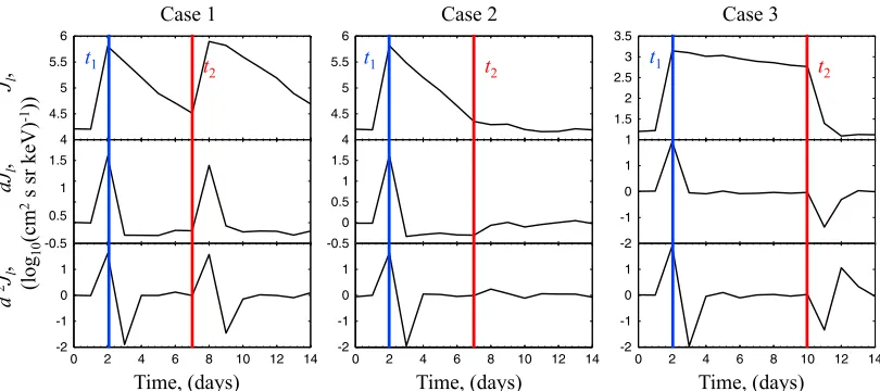
three different cases. These three cases are shown in Figure 2. In the first case (Figure 2 (left)), the decay of the electron flux is interrupted by a subsequent increase in flux. For the second case (Figure 2 (middle)), the flux levels off after decaying back to preevent values, similar to Figure 1f. In the third case (Figure 2 (right)), the electron flux decay is interrupted by a sudden dropout, akin to Figure 1d.

As mentioned above, each electron flux energy range was individually searched for local maxima to find the start of each decay period. Here as shown in all panels of Figure 2, dJ_l(t₁)must be positive, d2_J

l(t1+1)

must be negative and<d2_J

l(t1+2). This is true even if the buildup in fluxes happens over more than 1 day.

This occurs on day 2 for all cases in Figure 2. To find the end of the decay interval,t₂, the data between each consecutivet1were searched. If there is no significant changes in gradients within this interval, as in Case 1

of Figure 2, thent2is the point before the next increase in flux (day 7).

The end of the decay interval for Case 2 is largely influenced by noise since there is no large variation in dJ_l and d2_J

l. In Case 2,t2was defined byJl(t2)having a magnitude to within a threshold of the flux before the

increase, dJ_l(t₂+1) ∼0and d2_J

l(t2+1)is positive (it occurs on day 7). In the third case of Figure 2, the end of

the decay period occurs at the point before the dropout. This can be seen as a large change in gradient and was detected by|d2_J

6

5.5

5

4.5

4

6 3.5

3

2.5

2

1.5

1

1

0

-1

-2

1

0

-1

-2 5.5

5

4.5

4

1.5

1

0.5

0

-0.5

1

0

-1

-2 1.5

1

0.5

-0.5

1

0

-1

-2

0 2 4 6 8 10 12 14 0 2 4 6 8 10 12 14 0 2 4 6 8 10 12 14

Figure 2.Three cases showing the start,t₁, and end,t₂, of decay intervals in (top) the logarithmic electron flux,J_l, (middle) the first derivative,dJ_l, and (bottom) the second derivative,d2_J

l. Case 1: decay immediately followed by another increase in flux. Case 2: fluxes level off after decaying to preevent levels. Case 3: decay

interrupted by a dropout.

any fast dropouts from the study, including those observed in the storm main phase. This occurs on day 10 in Figure 2 (right).

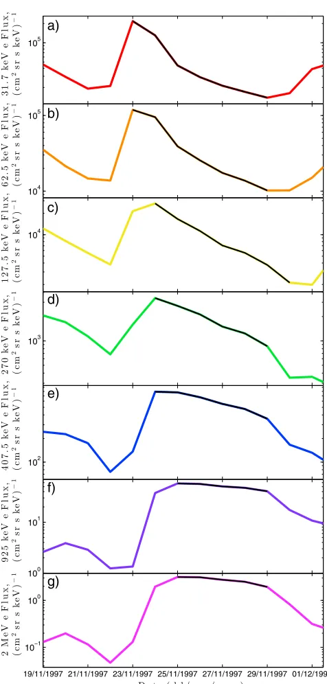
The data for each energy of electron flux were individually searched for decay intervals by employing the above criteria. The thresholds of the algorithm were tuned to a number of decays which would allow for a certain amount of noise resistance in detecting the events. All the decay intervals were then manually checked, removing any decays which seemed unreasonable, such as when the decay leveled off gradually (similar to Case 2) so that the end of the decay was not correctly detected, thus overestimating the lifetime. The number of decay intervals found was between 129 intervals for 24.1 keV and 255 for 1.3 MeV. Figure 3 displays an event of increased electron flux taking place between 19 November 1997 and 1 December 1997 for seven electron energies. The black line, for each of the seven plots, indicates the interval used to calculate the corresponding decay rate and lifetime.

In this event, the electron fluxes at low energies (Figures 3a and 3b) start a fast decay immediately after having peaked with a large gradient. In Figure 3d, the 172.5 keV flux starts to decrease with a less steep slope after it peaks. As the energy increases further, Figures 3e and 3f show that the gradient of this decay becomes smaller. Finally, for 2 MeV electrons shown in Figure 3g, the fluxes seem to plateau. This implies that the rate of depletion depends upon the energy range, decreasing with the increase of energy or, in other terms, that the electron lifetimes increase with increasing energy. For high energies such as 2 MeV, the loss rate is so small that the decrease of fluxes is not evident for this event, corresponding to very long lifetimes. The 2 MeV electron flux remain roughly constant until there is a dropout, which effects all electrons above 170 keV, during this event, on 29 November 1997. It can clearly be seen that the decay of electrons decreases as the energy increases relative to the magnitude of the increase. Moreover, the measured decays generally appear to be roughly exponential over all the selected intervals.

a)

b)

c)

d)

e)

f)

g)

Figure 3.The decay of the electron flux, depicted in a range of ener-gies: (a) 31.7 keV, (b) 62.5 keV, (c) 127.5 keV, (d) 270 keV, (e) 407.5 keV, (f ) 925 keV, and (g) 2.0 MeV. The black line superimposed on each electron flux displays the corresponding interval considered to calculate the decay and lifetime.

For each of the clearly identified decay intervals from the 20 years of LANL data, the decay rate,𝜆, of the electron flux,J, was calculated assuming an exponential form

J=Ae−𝜆t ₍₁₎

lnJ= −𝜆t+lnA (2)

whereAis a constant andtis the time. On this basis, the decay rate can then be found from a least squares fit for each clearly identified decay period:

𝜆=

n

n

∑

i=1

t(i)lnJ(i) −

n

∑

i=1

t(i)

n

∑

i=1

lnJ(i)

n

n

∑

i=1

t2_{(i) −} (_∑n

i=1

t(i)

)2

(3) The mean decay rate was then calcu-lated after averaging over all the clearly identified decay periods between 22 September 1989 and 13 December 2009 and the mean electron lifetime calculated from𝜏 = 1∕𝜆. Moreover, we also evaluated the 20% and 80% percentile of the distribution of decay rates𝜆, allowing us to provide an esti-mate of the observed variability around the mean decay rates and lifetimes (i.e., experimental error bars).

3. Electron Lifetime

Relation-ship With Energy

Figure 4 shows the relationships between the lifetime of electrons and their energy (red) as well as between electron decay rate and energy (black). The lifetime clearly increases propor-tionally to the logarithm of the energy up to 500 keV, where there is a discon-tinuity. Between 60 keV and 280 keV, one can see that there is a good agree-ment with lifetimes obtained from the SCATHA satellite atL∼6.1–6.5 in a pre-vious study [Su et al., 2012]. Analyzing storm events in 1979–1984,Baker et al. [1986] have also reported typical decay timescales of about 4 days for 3 MeV electrons atL=6.6which compare well with our results.

Figure 4.Electron decay rate versus electron energy (black) and electron lifetime versus electron energy (red).

It should be emphasized that very long lifetimes, larger than 10 days, actually correspond to less than 30% reduc-tions in electron fluxes over a typical decay interval of calculation of 4 days at GEO (see Figures 3f–3g and 1d). Furthermore, long lifetimes generally concern high energies (larger than 1 MeV) for which measured fluxes are considerably smaller than at lower energy (e.g., compare flux levels in Figures 3e–3g). Consequently, such long lifetimes should be much less accurately determined: relatively small fluctuations in the electron count rates can be sufficient either to suppress a small decay (for a positive fluctuation) or to significantly increase it (for a neg-ative fluctuation). Both these effects should actually concur to make long lifetimes (>10 days) much less likely to be spotted with the above discussed method.

4. Comparison With Analytical Lifetimes for Chorus-Induced Losses

The decay of energetic electron fluxes observed on satellites is the result of a competition between dif-ferent loss and source mechanisms. One of the most important loss processes is pitch angle scattering of electrons toward their loss cone (and precipitation in the atmosphere) due to wave-particle interactions. Relatively high amplitude chorus whistler mode waves are pervasive at GEO, which should generally make their resonant scattering of electrons one of the dominant processes. EMIC waves are most frequently observed during disturbed periods (such as the main phase of storms), near the plasmapause, or in regions of strongly decreasing plasma density less than one Earth radius away from the compressed plasmasphere, or (but seemingly more rarely) near the edge of plasmaspheric plumes formed during storms [e.g., see Thorne and Kennel, 1971;Carson et al., 2013;Usanova et al., 2013;Mann et al., 2014;Usanova et al., 2014, and references therein]. In contrast, our flux decays are measured only during rather moderately disturbed peri-ods (recovery phase) at GEO. In a first approach, it is therefore reasonable to consider only chorus-related wave-induced losses.

Energization by chorus waves of lower energy electrons up to the considered energy range is another important source process forE >100keV electron fluxes [Horne et al., 2005]. But the timescale for electron acceleration is usually longer than their lifetimes during low to moderate geomagnetic activity [Mourenas et al., 2014], which justifies a priori to consider only their losses by pitch angle diffusion after the flux decay has started. Actually, the beginning of the decay should correspond to the time when loss-limited energiza-tion has reached its peak and losses start to take over (e.g., see equaenergiza-tions (7)–(8) in the work byMourenas et al.[2014]). It is also worth noting that if such a source of energetic electrons by acceleration of lower energy ones were more important than losses during the observed flux decays, then the measured lifetimes would be increased as compared with chorus-induced losses alone. We shall see below that it is not the case. Con-sequently, energization is likely much weaker than losses during the observed decay periods, which agrees well with calculations performed byMourenas et al.[2014] during similarly not-too-disturbed periods such thatDst>−30nT atL∼7. Besides, radial diffusion of electrons is also very important at GEO [Brautigam and Albert, 2000;Shprits et al., 2008;Ozeke et al., 2014] and it will certainly influence the observed flux decays. Notwithstanding, we shall compare here the observed electron flux decays with analytical lifetime estimates obtained for losses by chorus waves alone. This should help us to assess whether additional loss or source mechanisms are necessary or not to explain the measured lifetimes—such as radial diffusion or other kinds of wave-particle interactions.

Thorne, 2010, and references therein]. In the present study, the measured lifetimes have been compared to the approximate analytical lifetime model derived byMourenas et al.[2012], because this work is the only one which accounts for a sensible proportion of whistler mode chorus waves propagating very obliquely with respect to the magnetic field. Recent statistics of 10 years of Cluster lower band chorus wave data have indeed shown that a significant portion of these waves is propagating near the resonance cone angle [Agapitov et al., 2013;Mourenas et al., 2014]. Numerical and analytical studies have demonstrated the impor-tant impact of these oblique waves and the resulting modification (generally reduction) of electron lifetimes [Mourenas et al., 2012;Artemyev et al., 2013a;Mourenas et al., 2014].

FollowingMiyoshi and Kataoka[2008], the decay of the electron flux should generally take place during peri-ods of moderate geomagnetic activity, after the end of the main phase of storms where energization usually occurs. During such nearly quiet periods, oblique waves are more present than during high geomagnetic activity [Agapitov et al., 2013;Mourenas et al., 2014]. Based on Cluster statistics at latitudes𝜆 ∼ 10◦–40◦ whenDst>−30nT, a small but influential portion (≥1%−5% typically) of the chorus wave intensityB2

wlies

in the very oblique range such that the wave normal angle𝜃 > 45◦. In this situation, electron pitch angle scattering rates are increased near the loss cone by the contribution of higher-order cyclotron resonances in addition to the fundamental one (the only contributing one for parallel waves). Then, one can use the ana-lytical lifetime estimate𝜏derived in case of a significant presence of oblique chorus waves [Mourenas et al., 2012;Artemyev et al., 2013a;Mourenas et al., 2014]. It is roughly valid for electron energiesE ∼ 20–30 keV to∼3MeV:

𝜏≈ 35

B2

w

𝛾(𝛾2−1)1∕2Ω_pe (4)

whereB_wis the bounce-averaged RMS wave amplitude in pT,𝛾is the Lorenz factor, andΩ_peis the electron plasma frequency. Assuming for simplicity a dipolar magnetic field and a typical 1∕L4_{plasma density profile,}

the plasma frequency to electron gyrofrequency ratio can be written approximately as

Ω_pe∕Ω_c≈5.78(L∕6.6) (5)

whereLis theLshell andΩ_cis the equatorial electron gyrofrequency and is approximately

Ω_c[days] ≈0.22(L∕6.6)−3 (6)

Therefore, the lifetime𝜏(in days) of an electron as a function of its energyE(in keV) and of chorus wave RMS amplitudeBw(in pT) reads as

𝜏[days] = 45[days⋅pT

2_{](E[keV]∕511+1)((E[keV]∕511+1)}2₋₁₎1∕2

(Bw[pT]L∕6.6)2

(7)

The above analytical expression can then be compared to the statistical mean lifetimes found in this study on the basis of satellite measurements.

Figure 5 displays the analytical lifetime for electrons at GEO (L=6.6) overlaid on the statistical electron life-times (red asterisks). Moreover, we also evaluated the 20% and 80% percentile of the distribution of electron lifetimes, allowing us to provide an estimate of the observed variability around the mean decay rates and lifetimes (i.e., experimental error bars). Here we have considered a mean wave amplitude of∼5 pT (black solid line) in agreement with statistical results from Cluster atL∼6–7 after averaging over latitudes𝜆∼0◦–40◦ during nearly quiet times such thatDst>−20nT [Mourenas et al., 2014]. A factor of 3 variance in the wave intensity around the average value has also been considered in rough concordance with Cluster obser-vations. Therefore, the upper limit on lifetimes (grey dashed line) corresponds toBw = 3pT while for its

lower limit we useBw = 9pT (black dashed line). Note that the average amplitude of chorus waves

gen-erally increases with latitude, while we used a constant (mean) amplitude here. Since the latitudinal range of resonance increases with energy (although much less for oblique waves), it could lead to slightly overes-timated (underesoveres-timated) lifetimes at high (low) energy when using a constant mean amplitudeBw∼5 pT.

Figure 5.Plot of electron lifetime versus electron energy. The red asterisks show the statistical results from the present study of LANL satellite data with the 20% and 80% percentile of the distribution of lifetimes, the black solid line shows theMourenas et al.[2012] analytical lifetime estimates for an average chorus wave amplitude of 5 pT, the dotted lines show a factor of 3 variance in chorus wave intensity around the mean, and the blue dots show the statistical results of electron decay times fromSu et al.[2012] for 45◦pitch angle and6.1<L≤6.5.

Figure 5 shows that for low electron energies, E∼24 keV to∼1 MeV, the statistical flux decay timescales roughly agree with the theoretical lifetime estimates derived for losses induced only by resonant interaction with average (nearly quiet time) chorus waves. Lifetimes due to scattering by chorus waves scale as𝜏∼𝛾p∼√Eto∼Ein this domain (corre-sponding to smaller pitch angle scattering of higher-momentum particles, e.g., see Moure-nas et al.[2012]), which remains comparable to the energy dependence of observed decay timescales as long asE <0.5MeV. Therefore, scattering by chorus waves seems to be the dominant loss factor forE < 0.5MeV elec-trons at GEO during weakly disturbed periods. However, forE>1.5MeV, the measured elec-tron lifetimes become sensibly smaller than the analytical estimates, while the energy dependence of analytical lifetimes becomes 𝜏∼Eto∼E2_{forE > 0.5MeV, clearly}

depart-ing from the very weak energy dependence of measured decay timescales. Some possi-ble explanations for these discrepancies are discussed below.

5. Discussion

We have already pointed out at the end of section 3 that long lifetimes (𝜏 > 10days) should be much less easily identified with the present methods and instruments than smaller lifetimes, as indicated by the increas-ing width of the error bars as energy increases above 1 MeV in Figure 5. Moreover, the lowest (24 keV) and highest (2 MeV) energy channels of the SOPA instrument could also be less accurate than the other ones (see explanations in section 2.1), while the 2.65 MeV channel is provided by another instrument (ESP). Thus, one should be very careful before drawing any definitive conclusions from the apparent discrepancy atE ∼2–2.7 MeV between analytically estimated and mean measured lifetimes.

One possible reason could be that the identified flux decays ofE ≥ 2MeV electrons may correspond to a higher mean geomagnetic activity than the flux decays identified at lower energies. Using higher cho-rus wave amplitudes corresponding to a slightly higher geomagnetic activityDst≈ −30 nT to−40 nT, i.e., Bw∼12–15 pT atL∼7 [Agapitov et al., 2013;Mourenas et al., 2014], the analytical lifetimes obtained above for

quiet time chorus wave-electron interaction [Mourenas et al., 2012] would be reduced by an additional fac-tor of 2 as compared to the lower bounds plotted in Figure 5, in much better agreement with observations forE > 1MeV. However, the meanDstover the considered decay periods actually varies from∼−20 nT to

∼−11 nT from low to high electron energies. Therefore, low-energy decay periods occur at times of slightly higher geomagnetic activity. This could be due to the increase of lower energy fluxes just after the storm main phase by injections and rapid heating, while the higher energies take 1 to 2 days more for their fluxes to increase by progressive acceleration of less energetic electrons. By this time, geomagnetic activity should have subsided slightly more toward quiet time levels.

indication that some additional and important physical processes are at work. In this regard, one impor-tant limitation of geosynchronous measurements stems from the fact that electron fluxes measured at GEO are close to the outer boundary of the radiation belt, especially in the night sector. As a result, the defor-mation of the geomagnetic field shape may have strong consequences on losses and radial transport of high-energy electrons (>1 MeV), while continuous injections of 10–100 keV electrons from the plasma sheet may reduce apparent losses (as measured by satellites) at low energies.

Let us first consider the well-known deformation of the geomagnetic field at GEO. It has recently been shown that using a realistic Tsyganenko 89 model for the magnetic field can decrease lifetimes ofE≥1MeV electrons atL∼ 6.6by about a factor of 2 whenKp ∼2, as compared to values obtained in a dipolar field, in the case of resonance with parallel chorus waves (see Figures 3c–3e in the work byOrlova and Shprits [2014]). Although the latter numerical calculations did not consider oblique waves, a similar reduction of high-energy electron lifetimes can be expected in this case because strong wave-particle coupling then occurs at higher latitudes, where the magnetic field gradient should be reduced on the dayside, widening the latitudinal range of scattering and decreasing lifetimes [Artemyev et al., 2013a]. However, the more likely situation, whereKp< 2, would probably lead to almost no reduction of the magnetic local time-averaged lifetimes. Another possibility would be an increased pitch angle diffusion of high-energy (>1 MeV) elec-trons caused by a strongly reduced magnetic field line curvature in the midnight sector at GEO during disturbed periods [Artemyev et al., 2013b]. But such effects are expected to occur at GEO only during impor-tant disturbances, while the present study focuses instead on moderately disturbed periods during the long recovery phase of storms. Finally, drift orbit bifurcations in the dayside-compressed geomagnetic field can lead to enhanced outward radial transport of energetic electrons toward the magnetopause even during relatively quiet periods [Ukhorskiy et al., 2014], which could accelerate energetic electron flux decreases at GEO.

Actually, radial diffusion probably plays a prominent role in the dynamics of electrons at GEO, potentially explaining the weak variation of observed lifetimes with energy, as suggested in the work bySu et al.[2012]. Many recent studies have demonstrated that there are positive (negative) radial gradients in low-energy (high-energy) electron phase space densities, with the transition from positive to negative gradient typically occurring for a magnetic moment𝜇≈200MeV/G, corresponding atL∼ 6.6toE ≈0.5–0.2MeV for pitch angles𝛼₀ ∼ 40◦–90◦[e.g., seeChen et al., 2005;Turner et al., 2012]. Radial diffusion should preferentially scatter particles toward lower phase space density. By continually replacing lost (or inward transported) low-energy electrons by new ones coming from higherLshells, it can make the observed lifetimes of elec-tronsapparentlylonger for energies lower thanE ∼ 0.5MeV. Conversely, by scattering higher-energy electrons toward the magnetopause (replacing energetic ones by less energetic, decelerated ones), it can reduce the measured lifetimes ofE>0.5MeV electrons.

A recent analytical formulation for the electric field radial diffusion coefficientDE

LLdue to ULF waves has

been provided byOzeke et al.[2014]. Let us assume a characteristic gradient scale of the phase space density ofΔL∼ Δr∕R_E ≈1atL=6.6(whereR_Eis Earth’s radius). The corresponding loss timescale𝜏_rdof high-energy (E>1MeV) electrons due to outward radial diffusion can be very roughly estimated as𝜏_rd≈ (ΔL)2_∕DE

LL≈20

days to 7 days forKp = 0toKp = 1(similar values obtain when usingBrautigam and Albert[2000] elec-tromagnetic radial diffusion coefficient). In addition, outward transport should be increased by drift orbit bifurcations at GEO [Ukhorskiy et al., 2014]. Thus, outward transport could really impose some additional upper limit𝜏 < 𝜏_rd ≈ 10days on the lifetimes ofE > 1MeV electrons at geosynchronous orbit. Numer-ical simulations of the Fokker-Planck diffusion equation including realistic magnetic field configurations, radial diffusion, chorus-induced losses, and realistic gradients in phase space density will be necessary in the future to investigate this point.

6. Conclusions

with energy. This increase is shown to be proportional to the logarithm of the energy up until approximately 500 keV, where the lifetime increase with energy starts to saturate.

For energies below 0.5–1 MeV, the mean statistical satellite results show a good agreement with the ana-lytical lifetime estimates obtained byMourenas et al.[2012] for losses due to resonant interaction between electrons and average (nearly quiet time) oblique chorus waves, since analytical lifetimes increase at a sim-ilar rate with energy. However, above 0.5–1 MeV, where the statistics show a change in proportionality between lifetime and energy, the discrepancy between the model and the statistics starts to grow, although the upper bounds of the measurement error bars still remain within the lower bounds of the model. The results of this study show that measured mean electron lifetimes increase only by a small amount with energy above 500 keV, while the lifetimes increase exponentially further in the analytical model. This could be intrinsically related to our method of identification of lifetimes, which could be biased toward lifetimes smaller than 10 days at high energy at GEO. Higher initial geomagnetic activity levels are probably required to produce higher-energy electron flux enhancements, which could lead to higher wave amplitudes and thus smaller analytical lifetimes than with average, quiet time amplitudes. Moreover,Orlova and Shprits [2014] have shown that using a realistic, nondipolar magnetic field, more appropriate during somewhat dis-turbed periods at GEO, could decrease lifetimes at high energies. Finally, it has been suggested that outward radial diffusion of high-energy electrons might further reduce their lifetimes at GEO, potentially explaining the “knee” in Figures 4–5. However, other mechanisms could also play a part.

References

Agapitov, O., A. Artemyev, V. Krasnoselskikh, Y. V. Khotyaintsev, D. Mourenas, H. Breuillard, M. Balikhin, and G. Rolland (2013), Statistics of whistler-mode waves in the outer radiation belt: Cluster STAFF-SA measurements,J. Geophys. Res. Space Physics,118, 3407–3420, doi:10.1002/jgra.50312.

Albert, J., and Y. Shprits (2009), Estimates of lifetimes against pitch angle diffusion,J. Atmos. Sol. Terr. Phys.,71(16), 1647–1652. Artemyev, A. V., D. Mourenas, O. V. Agapitov, and V. V. Krasnoselskikh (2013a), Parametric validations of analytical lifetime estimates for

radiation belt electron diffusion by whistler waves,Ann. Geophys.,31(4), 599–624.

Artemyev, A. V., K. G. Orlova, D. Mourenas, O. V. Agapitov, and V. V. Krasnoselskikh (2013b), Electron pitch-angle diffusion: Resonant scattering by waves vs. nonadiabatic effects,Ann. Geophys.,31(9), 1485–1490.

Baker, D. N., J. B. Blake, R. W. Klebesadel, and P. R. Higbie (1986), Highly relativistic electrons in the Earth’s outer magnetosphere: 1. Lifetimes and temporal history 1979–1984,J. Geophys. Res.,91(A4), 4265–4276.

Balikhin, M. A., R. J. Boynton, S. N. Walker, J. E. Borovsky, S. A. Billings, and H. L. Wei (2011), Using the NARMAX approach to model the evolution of energetic electrons fluxes at geostationary orbit,Geophys. Res. Lett.,38, L18105, doi:10.1029/2011GL048980.

Belian, R. D., G. R. Gisler, T. Cayton, and R. Christensen (1992), High-Z energetic particles at geosynchronous orbit during the Great Solar Proton Event Series of October 1989,J. Geophys. Res.,97(A11), 16,897–16,906.

Benck, S., L. Mazzino, M. Cyamukungu, J. Cabrera, and V. Pierrard (2010), Low altitude energetic electron lifetimes after enhanced magnetic activity as deduced from SAC-C and DEMETER data,Ann. Geophys.,28(3), 849–859.

Boynton, R. J., M. A. Balikhin, S. A. Billings, and O. A. Amariutei (2013a), Application of nonlinear autoregressive moving average exogenous input models to geospace: Advances in understanding and space weather forecasts,Ann. Geophys.,31(9), 1579–1589. Boynton, R. J., M. A. Balikhin, S. A. Billings, G. D. Reeves, N. Ganushkina, M. Gedalin, O. A. Amariutei, J. E. Borovsky, and S. N. Walker

(2013b), The analysis of electron fluxes at geosynchronous orbit employing a NARMAX approach,J. Geophys. Res. Space Physics,118, 1500–1513, doi:10.1002/jgra.50192.

Boynton, R. J., S. A. Billings, O. A. Amariutei, and I. Moiseenko (2013c), The coupling between the solar wind and proton fluxes at GEO,

Ann. Geophys.,31(10), 1631–1636.

Brautigam, D. H., and J. M. Albert (2000), Radial diffusion analysis of outer radiation belt electrons during the October 9, 1990, magnetic storm,J. Geophys. Res.,105(A1), 291–309, doi:10.1029/1999JA900344.

Carson, B. R., C. J. Rodger, and M. A. Clilverd (2013), POES satellite observations of EMIC-wave driven relativistic electron precipitation during 1998–2010,J. Geophys. Res. Space Physics,118, 232–243, doi:10.1029/2012JA017998.

Cayton, T. E., and M. Tuszewski (2005), Improved electron fluxes from the synchronous orbit particle analyzer,Space Weather,3, S11B05, doi:10.1029/2005SW000150.

Chen, Y., R. H. W. Friedel, G. D. Reeves, T. G. Onsager, and M. F. Thomsen (2005), Multisatellite determination of the relativistic electron phase space density at geosynchronous orbit: Methodology and results during geomagnetically quiet times,J. Geophys. Res.,110, A10210, doi:10.1029/2004JA010895.

Horne, R. B., R. M. Thorne, S. A. Glauert, J. M. Albert, N. P. Meredith, and R. R. Anderson (2005), Timescale for radiation belt electron acceleration by whistler mode chorus waves,J. Geophys. Res.,110, A03225, doi:10.1029/2004JA010811.

Horne, R. B., S. A. Glauert, N. P. Meredith, D. Boscher, V. Maget, D. Heynderickx, and D. Pitchford (2013), Space weather impacts on satellites and forecasting the Earth’s electron radiation belts with SPACECAST,Space Weather,11, 169–186, doi:10.1002/swe.20023. Mann, I. R., M. E. Usanova, K. Murphy, M. T. Robertson, D. K. Milling, A. Kale, C. Kletzing, J. Wygant, S. Thaller, and T. Raita (2014),

Spa-tial localization and ducting of EMIC waves: Van Allen Probes and ground-based observations,Geophys. Res. Lett.,41, 785–792, doi:10.1002/2013GL058581.

Meier, M. M., R. D. Belian, T. E. Cayton, R. A. Christensen, B. Garcia, K. M. Grace, J. C. Ingraham, J. G. Laros, and G. D. Reeves (1996), The Energy Spectrometer for Particles (ESP): Instrument description and orbital performance,AIP Conf. Proc.,383, 203–210, doi:10.1063/1.51533.

Meredith, N. P., R. B. Horne, S. A. Glauert, D. N. Baker, S. G. Kanekal, and J. M. Albert (2009), Relativistic electron loss timescales in the slot region,J. Geophys. Res.,114, A03222, doi:10.1029/2008JA013889.

Miyoshi, Y., and R. Kataoka (2008), Flux enhancement of the outer radiation belt electrons after the arrival of stream interaction regions,

J. Geophys. Res.,113, A03S09, doi:10.1029/2007JA012506.

Acknowledgments

The authors would like thank EPSRC, STFC, and ERC for financial sup-port. The authors would also like to acknowledge G. Reeves and the LANL group responsible for maintaining the in flight operations and processing the data archives for the SOPA and ESP instruments. The SOPA and EPS data used in this study are available at http://onlinelibrary.wiley.com/doi/ 10.1029/2010JA015735/suppinfo. The OMNIWeb interface provided the solar wind data, which was accessed from http://omniweb.gsfc.nasa.gov.

Mourenas, D., A. V. Artemyev, J.-F. Ripoll, O. V. Agapitov, and V. V. Krasnoselskikh (2012), Timescales for electron quasi-linear diffusion by parallel and oblique lower-band chorus waves,J. Geophys. Res.,117, A06234, doi:10.1029/2012JA017717.

Mourenas, D., A. V. Artemyev, O. V. Agapitov, and V. Krasnoselskikh (2014), Consequences of geomagnetic activity on energization and loss of radiation belt electrons by oblique chorus waves,J. Geophys. Res. Space Physics,119, 2775–2796, doi:10.1002/2013JA019674. Orlova, K., and Y. Shprits (2014), Model of lifetimes of the outer radiation belt electrons in a realistic magnetic field using realistic chorus

wave parameters,J. Geophys. Res. Space Physics,119, 770–780, doi:10.1002/2013JA019596.

Ozeke, L. G., I. R. Mann, K. R. Murphy, I. Jonathan Rae, and D. K. Milling (2014), Analytic expressions for ULF wave radiation belt radial diffusion coefficients,J. Geophys. Res. Space Physics,119, 1587–1605, doi:10.1002/2013JA019204.

Reeves, G. D., K. L. McAdams, R. H. W. Friedel, and T. P. O’Brien (2003), Acceleration and loss of relativistic electrons during geomagnetic storms,Geophys. Res. Lett.,30(10), 1529, doi:10.1029/2002GL016513.

Reeves, G. D., S. K. Morley, R. H. W. Friedel, M. G. Henderson, T. E. Cayton, G. Cunningham, J. B. Blake, R. A. Christensen, and D. Thomsen (2011), On the relationship between relativistic electron flux and solar wind velocity: Paulikas and Blake revisited,J. Geophys. Res.,116, A02213, doi:10.1029/2010JA015735.

Shprits, Y. Y., D. A. Subbotin, N. P. Meredith, and S. R. Elkington (2008), Review of modeling of losses and sources of relativistic electrons in the outer radiation belt II: Local acceleration and loss,J. Atmos. Sol. Terr. Phys.,70(14), 1694–1713.

Shue, J.-H., J. K. Chao, H. C. Fu, C. T. Russell, P. Song, K. K. Khurana, and H. J. Singer (1997), A new functional form to study the solar wind control of the magnetopause size and shape,J. Geophys. Res.,102(A5), 9497–9511.

Su, Y.-J., W. R. Johnston, J. M. Albert, G. P. Ginet, M. J. Starks, and C. J. Roth (2012), SCATHA measurements of electron decay times at 5_<L_≤8,J. Geophys. Res.,117, A08212, doi:10.1029/2012JA017685.

Summers, D., B. Ni, and N. P. Meredith (2007), Timescales for radiation belt electron acceleration and loss due to resonant wave-particle interactions: 1. Theory,J. Geophys. Res.,112, A04206, doi:10.1029/2006JA011801.

Thorne, R. M. (2010), Radiation belt dynamics: The importance of wave-particle interactions,Geophys. Res. Lett.,37, L22107, doi:10.1029/2010GL044990.

Thorne, R. M., and C. F. Kennel (1971), Relativistic electron precipitation during magnetic storm main phase,J. Geophys. Res.,76(19), 4446–4453.

Turner, D. L., V. Angelopoulos, Y. Shprits, A. Kellerman, P. Cruce, and D. Larson (2012), Radial distributions of equatorial phase space density for outer radiation belt electrons,Geophys. Res. Lett.,39, L09101, doi:10.1029/2012GL051722.

Turner, D. L., V. Angelopoulos, W. Li, M. D. Hartinger, M. Usanova, I. R. Mann, J. Bortnik, and Y. Shprits (2013), On the storm-time evo-lution of relativistic electron phase space density in Earth’s outer radiation belt,J. Geophys. Res. Space Physics,118, 2196–2212, doi:10.1002/jgra.50151.

Turner, D. L., et al. (2014), On the cause and extent of outer radiation belt losses during the 30 September 2012 dropout event,

J. Geophys. Res. Space Physics,119(3), 1530–1540, doi:10.1002/2013JA019446.

Ukhorskiy, A. Y., M. I. Sitnov, R. M. Millan, B. T. Kress, and D. C. Smith (2014), Enhanced radial transport and energization of radiation belt electrons due to drift orbit bifurcations,J. Geophys. Res. Space Physics,119, 163–170, doi:10.1002/2013JA019315.

Usanova, M. E., F. Darrouzet, I. R. Mann, and J. Bortnik (2013), Statistical analysis of EMIC waves in plasmaspheric plumes from Cluster observations,J. Geophys. Res. Space Physics,118, 4946–4951, doi:10.1002/jgra.50464.

Usanova, M. E., et al. (2014), Effect of EMIC waves on relativistic and ultrarelativistic electron populations: Ground-based and Van Allen Probes observations,Geophys. Res. Lett.,41, 1375–1381, doi:10.1002/2013GL059024.