On the mesoscale structure of surface wind and pressure fields near tornadic and nontornadic cold fronts

fields near tornadic and nontornadic cold fronts

.

White Rose Research Online URL for this paper:

http://eprints.whiterose.ac.uk/82617/

Version: Published Version

Article:

Clark, MR and Parker, DJ (2014) On the mesoscale structure of surface wind and pressure

fields near tornadic and nontornadic cold fronts. Monthly Weather Review, 142 (10). 3560

-3585. ISSN 0027-0644

https://doi.org/10.1175/MWR-D-13-00395.1

[email protected] https://eprints.whiterose.ac.uk/ Reuse

Unless indicated otherwise, fulltext items are protected by copyright with all rights reserved. The copyright exception in section 29 of the Copyright, Designs and Patents Act 1988 allows the making of a single copy solely for the purpose of non-commercial research or private study within the limits of fair dealing. The publisher or other rights-holder may allow further reproduction and re-use of this version - refer to the White Rose Research Online record for this item. Where records identify the publisher as the copyright holder, users can verify any specific terms of use on the publisher’s website.

Takedown

If you consider content in White Rose Research Online to be in breach of UK law, please notify us by

On the Mesoscale Structure of Surface Wind and Pressure Fields near Tornadic and

Nontornadic Cold Fronts

MATTHEWR. CLARK

Met Office, Exeter, Devon, United Kingdom

DOUGLASJ. PARKER

School of Earth and Environment, University of Leeds, Leeds, United Kingdom

(Manuscript received 10 December 2013, in final form 11 June 2014)

ABSTRACT

Observations from a mesoscale network of automatic weather stations are analyzed for 15 U.K. cold fronts exhibiting narrow cold frontal rainbands (NCFRs). Seven of the NCFRs produced tornadoes. A time-compositing approach is applied to the minute-resolution data using the radar-observed motion vectors of NCFR precipitation segments. Interpolated onto a 5-km grid, the analyses resolve much of the small-mesoscale structure in surface wind, temperature, and pressure fields. Postfrontal winds varied substantially between cases. Tornadic NCFRs exhibited a near-908wind veer and little or no reduction in wind speed on NCFR passage; these attributes were generally associated with large vertical vorticity, horizontal conver-gence, and vorticity stretching at the NCFR. Nontornadic NCFRs exhibited smaller wind veers and/or marked decreases in wind speed across the NCFR, and weaker vorticity, convergence, and vorticity stretching. In at least four tornadic NCFRs, increases in vorticity stretching preceded tornadogenesis. Doppler radar observations of two tornadic NCFRs revealed the development of misocyclones, some tornadic, during the latter stages of vorticity-stretching increase. The presence of cyclonic vortices only, in one case occurring at regular intervals along the NCFR, provides limited circumstantial evidence for horizontal shearing in-stability (HSI), though other vortex-genesis mechanisms cannot be discounted. Vorticity-stretching increases were associated with coherent mesoscale structures in the postfrontal wind field, which modified the cross-frontal convergence. Where cross-cross-frontal convergence was large, extremely narrow, intense shear zones were observed; results suggest that tornadoes occurred when such shear zones developed in conjunction with conditional instability in the prefrontal environment.

1. Introduction

Since the implementation of operational radar net-works, narrow, intense bands of rainfall have frequently been observed along cold fronts. These narrow bands have variously been termed ‘‘line convection’’ (Browning and Pardoe 1973;James et al. 1978;James and Browning 1979) and narrow cold frontal rainbands (NCFRs; e.g.,Houze et al. 1976;Houze 1993, 475–478; Jorgensen et al. 2003;

Gatzen 2011). The updrafts within NCFRs are associated with strong low-level convergence at the front (Browning

and Harrold 1970;Browning 1990;Wakimoto and Bosart 2000;Jorgensen et al. 2003).

NCFRs often exhibit along-line structure compris-ing line ‘‘segments’’ or ‘‘cores’’ separated by ‘‘gap’’ regions of lighter precipitation (e.g.,Hobbs and Biswas 1979; Matejka et al. 1980; Hobbs and Persson 1982;

Locatelli et al. 1995;Jorgensen et al. 2003). A number of different mechanisms have been invoked to explain the segment–gap structure. These include the modula-tion of the frontal updraft by vertical shear- and buoyancy-induced wavelike disturbances above the front (Kawashima 2007) and the modulation of the frontal updraft by trapped gravity waves, triggered by regions of stronger updraft along the cold front (Brown et al. 1999).

Locatelli et al. (1995) defined ‘‘large’’ gaps as those

Corresponding author address:Matthew R. Clark, Met Office, FitzRoy Road, Exeter, Devon, EX1 3PB, United Kingdom. E-mail: [email protected]

greater than 10–12 km in the alongfront direction, and suggested that they may be dynamically different from smaller gaps.

Intense NCFRs often produce damaging wind gusts and short-lived, nonsupercell tornadoes (e.g.,Carbone 1982,1983;Elsom 1985;Meaden and Rowe 1985;Turner et al. 1986;Grumm 2000;Kobayashi et al. 2007;Sugawara and Kobayashi 2009;Smart and Browning 2009;Clark 2013). Doppler radar data have shown that NCFR tor-nadoes and other instances of localized wind damage are often associated with misoscale vortices of diameter 1–4 km (sometimes called ‘‘misocyclones’’ or ‘‘meso-vortices’’) that form along the zone of abruptly veering winds and associated strong vertical vorticity at the leading edge of the line (Carbone 1982,1983;Kobayashi et al. 2007;Clark 2012). As the misocyclone evolves, the NCFR usually develops a miso- to meso-g-scale pertur-bation or inflection point (e.g.,Carbone 1982;Smart and Browning 2009). Small line gaps (usually ,10 km in alongfront length) sometimes evolve near mature and decaying misocyclones (e.g., Grumm and Glazewski 2004;Lane and Moore 2006;Smart and Browning 2009). The association between line gaps and misocyclones is by no means unique, however, owing to the variety of other mechanisms that may be responsible for the generation of gaps.

Horizontal shearing instability (HSI;Haurwitz 1949;

Miles and Howard 1964) has commonly been invoked to explain the formation of NCFR misocyclones (e.g.,

Matejka et al. 1980; Carbone 1982, 1983; Smart and Browning 2009) and therefore is one possible mecha-nism for the development of line gaps. HSI results in the rollup of a sheet of vorticity into discrete, like-signed vortices. Smart and Browning (2009) used a high-resolution model simulation to investigate misocy-clones in a tornadic NCFR over northern England, from which they inferred the occurrence of vortex-sheet rollup. In this and other observed cases (e.g.,Carbone 1983), misocyclones and associated tornadoes occurred in mature NCFRs, which did not appear to exhibit any ob-vious intensification prior to tornadogenesis. However, the onset of HSI as a mechanism for the generation of the misocyclones might imply that the magnitude of ver-tical vorticity along the NCFR had increased over time, thereby rendering a formerly stable frontal shear line unstable to HSI. The onset of HSI could alternatively be associated with a reduction in alongfront deformation strain, which is known to suppress barotropic instability (e.g.,Dritschel et al. 1991;Bishop and Thorpe 1994;Dacre and Gray 2006).Dritschel et al. (1991)show that a mod-erate ‘‘frontogenetic’’ strain field, of order 0.25 times the magnitude of vorticity, will suppress the instability. Therefore, either a reduction in the strain, or an increase

in the vorticity, could allow a marginal situation to be destabilized. Although the process of ‘‘frontal collapse’’ and NCFR development have been studied (e.g., Koch and Kocin 1991), the process of misocyclone develop-ment in situations of increasing vertical vorticity along mesoscale sections of an already-mature NCFR have not been explored. Furthermore, to the best of the authors’ knowledge, no in situ observations of vertical vorticity increases preceding misovortex and tornadogenesis along NCFRs have been made.

An alternative mechanism for the generation of misoscale vortices along linear convective systems is the tilting mechanism, in which initially horizontal vorticity is tilted into the vertical by localized updrafts or downdrafts along the line. The horizontal vorticity may be associated with either the ambient vertical wind shear or buoyancy gradients across the gust front. The tilting mechanism has been shown to be re-sponsible for vortex genesis in quasi-linear convective systems forming in environments containing substantial buoyant instability (e.g., Trapp and Weisman 2003;

Weisman and Trapp 2003). Misocyclones may also form when horizontal vorticity associated with horizontal convective rolls is tilted into the vertical, where the rolls intersect the front (Atkins et al. 1995;Marquis et al. 2007).

A limitation in previous observational studies of the low-level structure of NCFR-bearing cold fronts has been the paucity of surface data, both spatially and temporally. In this paper, we use a time-compositing analysis of 1-min data from the U.K. automatic weather station network to analyze a set of 15 NCFRs at a spatial resolution of;5 km. Seven of these NCFRs produced at least one tornado. The aims of the study are threefold. A primary aim is to document some of the smaller-mesoscale structure in surface wind, tem-perature, and pressure fields near to NCFRs, and to document the variability in structure between cases. A second aim is to quantify the horizontal convergence and vertical vorticity across the NCFR, and to reflect on how the observed evolution of these parameters may bear on theories of vortex genesis along NCFRs. A third aim is to demonstrate the utility of the 1-min-resolution surface data for the construction of detailed fields of sur-face parameters. The time-compositing technique is de-scribed in section 2. The results are presented and discussed insections 3,4, and5. Conclusions are given in

section 6.

2. Method

resolution. A total of 15 cold fronts exhibiting an ex-tensive, well-marked NCFR occurred within the period for which archived minute-resolution data were available. All the cold fronts were associated with extratropical cy-clones moving from the west or northwest across, or to the north of the United Kingdom (Fig. 1). Although no strict selection criteria were applied, all analyzed NCFRs had a horizontal extent exceeding 100 km in the along-line direction, a lifetime exceeding 4 h, and core rainfall rates generally exceeding 8 mm h21_{(at 1-km resolution). The}

Tornado and Storm Research Organization’s (www.torro. org.uk) tornado database was used to classify lines as tornadic and nontornadic, using the method of Clark (2013).

The 1-min-resolution data were processed onsite at Met Office surface stations (Green 2010), and sent back to the Met Office headquarters in near–real time, where they are archived for a period of 1 year. The archive permits analysis of the high-resolution surface data en masse for the selected NCFR cases. By converting the minute data into equivalent spatial locations (‘‘time-compositing’’ analysis), using an observed system ve-locity, it is possible to derive detailed surface fields from the time series of data observed at each station. For each NCFR, a representative system velocity was calculated from sequences of composite radar rainfall imagery. Since individual line segments move with a component of motion in the alongfront direction (James and Browning 1979), the mean velocity of several segments over a period of at least 2 h was used, rather than that of the NCFR as a whole. Systematic variations in ground-relative segment velocity did occasionally occur over large distances (on the order of 1022103km) in the alongfront direction (e.g., in cases where the orientation of the front varied substantially and systematically along the front). The analysis domain was limited to 49.88– 54.58N, 3.48W–3.18E in these cases, in order to limit the differences in segment velocity across the domain. Where the NCFR was composed of a single, continuous line, the velocity of individual ‘‘elements’’ could be in-ferred from the movement of perturbations in the NCFR, such as inflection points associated with mi-soscale or memi-soscale waves.

The time-composited data were interpolated onto a regular grid using Delaunay triangulation, with grid spacing of 5 km35 km at the center of the domain. Plots of surface temperature, pressure and wind vec-tors were generated from the interpolated fields. The 5-km grid was found to be optimal after experimen-tation with various other grids of grid length between 1 and 20 km. At larger grid lengths, much of the detail associated with the larger segment-gap structure of the NCFRs (on the order of tens of kilometers in the

alongfront direction) was lost; at smaller grid lengths, artifacts resulting from the time-compositing analysis technique reduced the clarity of the plots in some areas, and tended to mask some of the resolved detail at smaller scales. Given that the full U.K. network comprises

;270 stations, the 640-min integration period yields

;21 600 data points for parameters measured at all sites. For the subset of stations used in the analyses of tem-perature, winds, and pressure, the mean horizontal spacing of data points is 3.4, 4.3, and 4.8 km, respectively (though the density of points is variable across the do-main). For the analysis of horizontal winds, from which derivative quantities are calculated, the mean station spacing to grid spacing ratio equals 1.17. This is some-what larger than the optimum ratio of 0.3–0.5 as sug-gested byKoch et al. (1983); however, the experiments with different gridbox sizes suggested that grid lengths of less than 5 km produced noisy derivative fields in some parts of the domain, perhaps owing to the vari-ability in the density of data points across the domain. The 5-km grid, therefore, represents a compromise so-lution, being large enough to avoid noisy derivative fields over the whole domain, but small enough to en-sure that the cross-frontal gradients are adequately represented.

Analyses were produced at a temporal resolution of 5 min as the NCFR traversed the analysis domain. Gradients of the uandy winds were calculated, from which the relative vertical vorticity jrel and horizontal

convergenceCwere obtained. The product ofjrelandC

gives vorticity stretching (hereafter stretching), which describes the rate of change of relative vertical vorticity associated with the divergence of the horizontal wind field. Stretching was calculated over all grid points within the domain. The domain-maximum values of conver-gence, vorticity, and stretching were also calculated every 5 min during the period in which the NCFR lay within the analysis domain, in order to identify any temporal trends in the magnitude of these parameters.

Time-compositing techniques have previously been used in mesoscale analyses of surface fields near torna-dic storms, mesoscale convective systems, and intense extratropical cyclones (e.g.,Fujita 1955,1958;Browning and Hill 1984; Browning 2004). Some authors (e.g.,

analysis. Here, we choose the simpler time-compositing analysis, because it retains the very high resolution of data in the direction normal to the system velocity, thereby permitting maximum possible resolution of the cross-frontal gradients in surface parameters, which are the primary focus of this investigation.

The central assumption of the time-compositing analysis is that the system-relative structure has only small variations over the time-compositing period (i.e., the system is steady state, or nearly so), and therefore, time variations in parameter values observed at a single point can be assumed to equate to spatial variations in the direction of the system motion. Radar data suggest that, on the mesoscale and larger scales, the steady-state assumption is valid over the640-min period chosen for the time compositing. The640-min period also had the advantage that, given the system speeds observed in the set of cases analyzed, it provided a good coverage of data points, while generally avoiding excessive overlap be-tween data points obtained from neighboring stations (Fig. 2).

Koch and O’Handley (1997) showed that errors resulting from uncertainties in estimation of the system velocity only lead to acceptably small analysis errors if the time-compositing period is restricted to

,55 min and the uncertainty in system velocity is no larger than 25%. Since the640-min period used here does not adhere toKoch and O’Handley’s (1997) tem-poral criterion, analyses were conducted using a shorter time-compositing period of 620 min for three cases (chosen because they exhibited large changes, during the analysis period, of vorticity stretching, as will be discussed subsequently), and results were compared with those obtained using the longer compositing pe-riod. Results showed that peak values of vorticity stretching were systematically larger with the longer integration period; for example, peak values obtained using the 640-min period were 115%–150% of the corresponding values obtained using the 620-min pe-riod. However, the overall trends in the vorticity stretching over the period that the NCFR crossed the analysis domain, and the time at which the largest values occurred, were relatively insensitive to the change in time-compositing period; for example, the difference in the timing of peak stretching was 18 min, on average, for the three cases.

Qualitatively, the analyses of measured parameters (temperature, pressure, and wind) appeared to be de-graded in some areas when using the shorter time-compositing period, owing to the existence of larger data gaps in a few parts of the domain, which necessi-tated interpolation over larger areas (a consequence of the shorter line of data points obtained from individual

stations when using the shorter time-compositing pe-riod). Since the relative values of the derived parameters and their temporal evolution showed little sensitivity to the choice of time-compositing period, and because the analyses were qualitatively more coherent with the longer compositing period, the640-min period was used for subsequent analysis.

the exact alongfront location of the individual peaks in vorticity and horizontal convergence was influenced by the choice of segment velocity, the overriding mesoscale structure of these fields in the alongfront direction was unaffected. Furthermore, temporal trends in domain-maximum values of vertical vorticity, horizontal con-vergence, and vorticity stretching were not significantly affected by the choice of system velocity. For example, on average over the three cases, the magnitude of in-dividual peaks in vorticity stretching varied by 13%, and their time of occurrence by 15 min, between analyses generated using the smallest- and largest-observed seg-ment speeds.

To minimize the effects of systematic observation biases at specific sites, a number of corrections were made to the data. First, temperature was corrected for altitude assuming a saturated adiabatic lapse rate. Radiosonde data indicated near-surface lapse rates were generally between the dry and saturated adia-batic lapse rates; therefore, the saturated adiaadia-batic assumption would lead to a small underestimate of near-sea-level temperatures (the resulting error should always be less than 0.58C for the;80% of sites located #150 m above sea level). The mean wind speed over all sites and all NCFR cases was calculated. This was divided by the mean wind speed at each

station. A correction factor was thus obtained for each station, which was applied to all wind speed data. In practice, these corrections could not remove all site-specific bias, and initial results showed that it was also necessary to exclude wind observations from sites lo-cated at $400-m altitude. Additionally, data from a small number of very sheltered and very exposed sites (such as cliff-top sites) were excluded. The final subset of sites comprised approximately 267 temper-ature stations, 164 wind stations, and 132 pressure stations (the exact totals vary slightly from case to case, because new sites are continually being added to the network).

3. Comparison and synthesis of 15 cases

a. Temperature, wind, and pressure

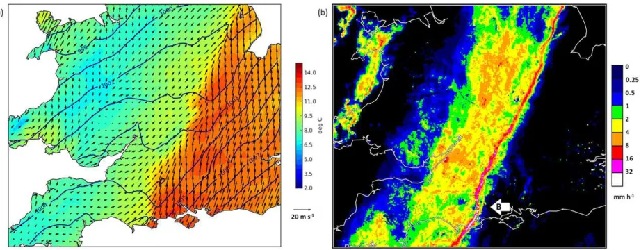
period that the front traversed the analysis domain). Over much of northern England, the NCFR (marked in Fig. 3b) was embedded within a wide cold frontal rainband of width ;100 km (the western edge of the latter is located close to the west coast of northern England at analysis time). The NCFR was moving rapidly eastward (at;18 m s21in the direction normal to the front), while individual NCFR segments were moving toward the east-northeast. Comparison with wind profiles obtained from radiosonde and wind profiler data showed the segment motion vector was orientated;308clockwise of the mean prefrontal wind vector in the 0.5–2.5 km above ground level layer, and moved with ;60% of the mean wind speed over the same layer (the mean values of these parameters, for all events, are 268 and 68%, respectively). The cold front is apparent in the sharp temperature gradient [.2.08C (5 km)21 in the cross-front direction], near-908wind veer and abrupt turning of the isobars across the sharp trough axis, the latter accentuated by a 2–3-hPa pressure surge over 10 km in the cross-front direc-tion, immediately to the rear of the front. A number of details are resolved on the small mesoscale, including the eastward-bulging configuration of the front near the center of the domain, the very sharp gradients in temperature and wind direction near the apex of the bulge, and the comparatively weak gradients over the southern parts of the domain, where the frontal wind veer and temperature decrease are spread over a zone ;40 km wide in the cross-front direction. A smaller region of weaker cross-front gradients is also apparent to the north of the line bulge, in the area south of the 990-hPa contour label. Comparison with rainfall imagery shows that the sharpest gradients are

generally associated with the strongest line segments, while the areas of weaker cross-front gradients tend to be associated with weaker segments, or line gaps. This is consistent with previous observations of NCFRs which have shown the strongest cross-frontal gradi-ents in temperature, pressure, and winds to be asso-ciated with line segments, with much weaker gradients near NCFR gap regions (e.g., James and Browning 1979).

Another intense NCFR affected the United King-dom on 22 November 2012 (Fig. 4). The surface cold front was advancing from west-northwest to east-southeast with a front-normal speed of 6.7 m s21_.

However, individual elements within the NCFR were moving toward the northeast (the motion vector of elements was orientated 188 clockwise of the mean prefrontal wind vector in the 0.5–2.5 km above ground level layer). Again, the surface cold front and associ-ated NCFR are marked by a sharp gradient in tem-perature [generally .1.58C (5 km)21]. However, the configuration of the wind and pressure field is different from that on 29 November 2011. The wind veer is smaller (generally ;458) and the wind speed drops substantially immediately behind the front. The ex-tensive region of lighter winds to the rear of the front is associated with a region of weak pressure gradients, of width ;150 km in the front-normal direction, con-trasting markedly with the strong pressure gradients to the east of the front. The postfrontal pressure surge is weak, or absent (generally#1 hPa). A small region of stronger postfrontal winds is evident over Dorset, En-gland, which corresponds to the location of a line bulge (marked by an arrow inFig. 4b), again demonstrating that the time-compositing analysis is able to resolve FIG. 4. (a) 5-km gridded temperatures, winds, and pressure. (b) Composite radar rainfall imagery for 2000 UTC 22 Nov 2012 (type-B

some of the small-mesoscale features along the front. The localized, marked undulation in the position of the maximum temperature gradient farther northeast along the front is not reflected in the radar-observed NCFR, and is likely an artifact of the time-compositing analysis; a consequence of the fact that the motion of the NCFR was not entirely uniform along its length. This feature highlights the fact that small features in the time-composited and interpolated fields need to be confirmed in other datasets, or by consideration of their temporal coherence, before they can be analyzed with confidence.

Similar plots were produced for the remainder of the 15 NCFRs selected for analysis. In all cases, the NCFR was marked by a narrow (;5–10 km wide) zone of strong temperature gradients (domain-maximum values exceeded 0.58C km21 over 5 km in the cross-front direction; see Table 1). Prefrontal winds were reasonably homogenous over the domain, and in all cases were orientated nearly parallel to (generally making an angle of less than 208with) the front. In contrast, the postfrontal wind and pressure fields exhibited marked variability from case to case and, sometimes, within the analysis domain for in-dividual cases. Estimates of the mean pre and post-frontal wind speeds were obtained from contour plots of wind speed, generated by time-compositing and interpolation of the data onto a 5-km grid (i.e., in the same way that the temperature, pressure, and wind vector plots inFigs. 3aand4awere generated). These analyses were produced at 10- or 20-min intervals over the period that the NCFR traversed the analysis do-main (larger intervals being used for events in which the cold front was slower to traverse the domain). Mean values of pre- and postfrontal wind speeds were estimated by taking the average of the maximum and minimum values observed within 30 km of the front (as defined by the zone of maximum wind veer) at each analysis time. Event averages were then ob-tained by taking the mean values over all analysis times. The mean postfrontal wind speeds and the range of values observed in each case are given in

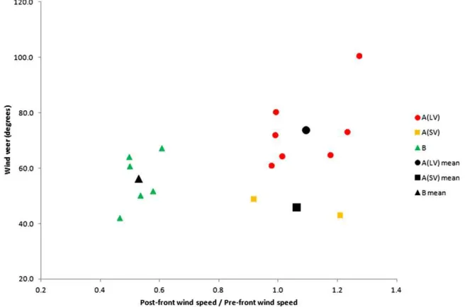
Table 1. The mean cross-frontal wind veer magnitude was analyzed from the raw data by calculating the maximum wind veer over 10 min at each site and taking the mean over all stations within the domain in each case. In this small sample, the cases appear to occupy distinct regions in the parameter space de-scribed by the ratio of prefrontal to postfrontal wind speed versus the wind-veer magnitude (Fig. 5). For the purposes of the subsequent analysis it is useful to split the cases into two types: cases in which the postfrontal wind speed remains strong, relative to the

prefrontal wind speed (hereafter called type A), and cases in which wind speeds decrease markedly on frontal passage (type B). The type-A cases may be subdivided according to the magnitude of wind veer across the front. The three resulting types are as follows:

d Large-veer, strong postfrontal winds (‘‘type A

LV’’;

circles inFig. 5): little or no decrease in wind speed postfront (an increase occurring in some cases), large wind veer (..458and locally near 908) and marked postfrontal pressure surge (as inFig. 3).

d Small-veer, strong postfrontal winds (‘‘type A

SV;’’

squares inFig. 5): little or no decrease in wind speed postfront, small wind veer (generally#458–508) (e.g., the NCFR of 8 December 2011;Fig. 6)

d Weak postfrontal winds (‘‘type B’’; triangles in

Fig. 5): marked decrease in wind speed immediately postfront (postfrontal wind speed ,50%–60% of prefrontal wind speed), variable magnitude of wind veer, and little or no postfrontal pressure surge (as in

Fig. 4).

Analysis of a much larger sample of cases would be required in order to ascertain whether the separation of cases among categories A and B in Fig. 5is gen-erally true of NCFRs. Furthermore, the NCFRs ana-lyzed herein sometimes exhibited variation in type along their length, and sometimes evolved from one type to another, as will be discussed. The types allocated here (and the values shown in Fig. 5) are indicative of the dominant type in each case, assessed over the whole analysis domain. Consideration of Fig. 5, and the sub-sequent analysis of the 15 cases, indicates that the dif-ferent types have some relevance to the dynamics of each NCFR.

Table 1lists the type of each NCFR analyzed, with the values of various parameters relating to the wind and pressure fields in each case. All of the tornadic NCFRs were of type ALV, at least along the part of the

NCFR that the tornadoes occurred. The 12 September 2012 case differed from other ALVcases in that

pre-frontal winds were weak. However, in common with the other ALV events, this NCFR possessed a large

wind veer (locally near 908) and an abrupt pressure surge immediately to the rear of the line. The synoptic situation on 12 September 2012 was atypical for a NCFR, and satellite and radiosonde data suggest that it may have been an example of a split cold front (e.g.,

TABLE1. Attributes of the 15 analyzed NCFRs (see main text for details). Numbers in parentheses indicate the observed ranges of the line-normal wind speeds postfront (within an area bounded by the NCFR and an imaginary line located 30 km to the rear of, and parallel to, the NCFR). The mean values of each parameter for tornadic (ALV) and nontornadic (ASVand B) cold fronts are given in the last two rows. Boldface type indicates that the differences between tornadic and nontornadic values are significant at the 95% level; italicized type indicates differences are significant at the 99% level. NS denotes values that could not be calculated because of a lack of representative sounding data. Date Type Tornadic [yes (Y)/no (N)] Mean domain-maximum convergence

(1023_s21₎

Mean domain-maximum

vorticity (1023_s21₎

Mean domain-maximum stretching (1025_s22₎

Absolute maximum stretching (1025_s22₎

0–1-km

N2

s (s2 2_,

1024₎ prefront

Prefrontal CAPE (J kg21₎

0–2.5-km above ground

level bulk shear magnitude

(m s1₎

29 Nov 2011 ALV Y 1.71 1.82 0.21 0.45 20.798 33 23

8 Dec 2011 ASV N 1.34 1.18 0.09 0.14 1.848 0 29

11 Dec 2011 B N 0.77 0.87 0.04 0.10 0.547 59 19

12 Dec 2011 ASV N 1.24 1.25 0.08 0.24 1.131 1 25

23 Dec 2011 ALV Y 1.29 1.53 0.13 0.48 20.090 14 21

3 Jan 2012 ALV Y 1.87 1.78 0.19 0.40 20.478 14 28

25 Jan 2012 B N 0.87 0.93 0.05 0.13 0.337 11 17

29 Aug 2012 ALV Y 0.99 1.06 0.07 0.25 21.084 39 14

12 Sep 2012 ALV Y 0.97 1.13 0.05 0.09 20.102 187 13

31 Oct 2012 B N 0.82 0.94 0.04 0.07 21.174 123 19

22 Nov 2012 B N 0.98 0.82 0.04 0.10 20.488 33 24

29 Dec 2012 B N 0.87 0.99 0.06 0.17 0.151 0 13

29 Jan 2013 B N 0.96 1.16 0.07 0.18 0.026 0 28

18 Dec 2013 ALV Y 1.78 1.91 0.20 0.40 20.373 16 36

25 Jan 2014 ALV Y 1.57 1.54 0.14 0.32 NS NS 27

Tornadic mean

1.45 1.54 0.14 0.34 20.488 51 23.1

Nontornadic mean

0.98 1.02 0.06 0.14 0.297 28 21.8

Date Type Tornadic [yes (Y)/no (N)] Largest temperature gradient over 5 km in

cross-front direction (8C km21 )

Largest postfront

pressure increase over 10 km in cross-front direction (hPa)

10-min wind veer (8)

(mean of all sites within domain) Postfrontal wind speed/ prefrontal wind speed Mean line-normal wind speed postfront

(m s21 )

Rate of advance of NCFR in

direction normal to its length (m s21

)

29 Nov 2011 ALV Y 0.98 3.30 80.4 0.99 12.5 (10–15) 17.7

8 Dec 2011 ASV N 0.87 2.17 49.0 0.92 7 (6–8) 12.7

11 Dec 2011 B N 0.72 0.95 42.2 0.47 3.5 (2–5) 10.8

12 Dec 2011 ASV N 0.95 2.07 43.0 1.21 8.5 (7–10) 15.7

23 Dec 2011 ALV Y 0.73 2.01 100.8 1.27 11.5 (9–14) 14.7

3 Jan 2012 ALV Y 1.34 3.87 61.1 0.98 14.5 (12–17) 17.9

25 Jan 2012 B N 0.70 1.07 67.6 0.61 4.5 (3–6) 8.3

29 Aug 2012 ALV Y 0.91 1.94 64.4 1.01 6.5 (5–8) 13.4

12 Sep 2012 ALV Y 0.53 1.02 73.3 1.23 6 (4–8) 13.3

31 Oct 2012 B N 0.89 0.40 64.3 0.50 2.5 (1–4) 5.2

22 Nov 2012 B N 0.76 1.87 52.0 0.58 3.5 (1–6) 6.7

29 Dec 2012 B N 0.59 1.60 50.3 0.53 5 (2–8) 9.1

29 Jan 2013 B N 0.69 0.74 60.9 0.50 4.5 (2–7) 9.4

18 Dec 2013 ALV Y 1.00 3.12 72.1 0.99 12.5 (3–22) 21.4

25 Jan 2014 ALV Y 1.17 3.00 64.8 1.17 11.5 (3–20) 22.6

Tornadic mean

0.95 2.61 73.8 1.09 10.7 17.3

Nontornadic mean

fronts (Browning and Pardoe 1973; Browning et al. 1998), and as observed in the other NCFR cases ana-lyzed herein.

b. Vorticity, convergence, and stretching

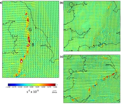
The NCFR of 29 November 2011 was marked by a line of large vertical vorticity, horizontal convergence, and vertical vorticity stretching (Fig. 7a; domain and analysis time are as in Fig. 3). Maximum values of vorticity and convergence on the 5 km35 km grid exceed 23

1023s21and stretching locally exceeds 0.2531025s22.

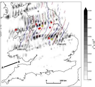
A sequence of stretching, analyzed at 15-min intervals during the period in which the NCFR crossed the country (Fig. 8), reveals persistent alongfront variations in the intensity of stretching. These variations occur on at least two, distinct horizontal scales. First, there are variations on scales close to the typical alongfront spacing of observing stations (;15–30 km). Second, there are variations on the mesoscale (;50–200 km). For example, large stretching values (.;0.0131025s22) are evident over many parts of the north Midlands and northern England, but such large values are generally absent over FIG. 5. Scatterplot of cross-frontal wind veer vs the ratio of the wind speeds postfront to

prefront. Categories ALV, ASV, and B (circles, squares, and triangles, respectively) are de-scribed insection 3aof the main text.

southern England. The mesoscale variations can be considered realistic, as demonstrated by the correspon-dence between the larger-scale segment-gap structure as observed by radar (Fig. 3b), and the areas of larger and smaller stretching. For example, the swathe of large stretching values over northern England corresponds to the track of a mesoscale bulge in the NCFR, the apex of which was located due west of the Humber Estuary at the analysis time (marked ‘‘B’’ inFig. 7a). The; 30–40-km-wide NCFR gap located to the north of this bulging segment is reflected by an along-line minimum in the stretching (marked ‘‘G’’ inFigs. 7aand8). The mesoscale regions of large stretching persist for several hours and extend over distances comfortably exceeding the length of the640-min line of data points obtained from any one surface station (the latter is shown inFig. 8). Conversely, the smaller-scale variations are at least partly a conse-quence of the distribution of observing stations; values are largest near the lines of data points obtained from individual stations, while lower values exist where there are larger gaps in the observing station distribution in the

alongfront direction, where interpolation over greater distances reduces the effective resolution of the data. Therefore, the precise locations of the individual tracks of largest vorticity stretching should not be taken literally. However, the peak values of stretching within these tracks may be considered indicative of values that might be obtained more generally, within the mesoscale swathes of larger stretching, given sufficient density of surface stations in the alongfront direction. Therefore, while the tornado and wind damage locations do not always lie along the individual tracks of largest stretching, they do all lie within the mesoscale corridors of generally large stretching values. It is the mesoscale variations in stretching magni-tude along the NCFR and the temporal evolution of the peak values of stretching within these mesoscale regions of large stretching that are of interest in this study.

For the type-B NCFR of 22 November 2012, local maxima in convergence and vorticity are again apparent in some places along the NCFR (not shown); how-ever, the maximum values are only around 30%–50% of those on 29 November 2011 (domain maximum values FIG. 7. Vorticity stretching fields at (a) 1430 UTC 29 Nov 2011, (b) 2000 UTC 22 Nov 2012, and (c) 1530 UTC 8 Dec

of 0.5–1.25 3 1023s21). The location of the front is barely discernible in the stretching field (Fig. 7b), since values along the front are not substantially larger than elsewhere within the analysis domain. In the type-ASV

NCFR of 8 December 2011, the convergence is locally large and maximum values are comparable with those observed on 29 November 2011 (.;1.5 3 1023

s21

). However, the peak values of vorticity of;1.331023

s21

are lower than on 29 November 2011, probably owing to the smaller veer (;408–508vs;808–908). Consequently, maximum values of stretching are intermediate between those of the type-ALV and type-B cases. The largest

vorticity and stretching are associated with areas in which postfrontal winds are locally more veered (Fig. 7c).

When comparing domain-maximum stretching for all 15 NCFRs (Table 1), five cases stand out as having rel-atively large values: 29 November 2011, 23 December 2011, 3 January 2012, 18 December 2013, and 25 January 2014. These cases are all of type ALV. The remaining two

ALVcases (29 August and 12 September 2012) exhibited

stretching values comparable to the ASVand B events.

In both these cases, prefrontal and postfrontal winds were weak compared to those in other ALV cases,

re-sulting in comparatively weak vorticity despite the

;608–708wind veer and lack of reduction in wind speed on frontal passage.

c. Temporal trends in convergence, vorticity, and stretching

The 50-min-mean values of domain-maximum vor-ticity and stretching were calculated for all 12 NCFRs over the period that each NCFR traversed the analysis domain. In at least five of the seven tornadic NCFRs, tornadogenesis was preceded by a 1–2-h period of in-creasing vorticity stretching (Fig. 9a). One exception was the 12 September 2012 case, in which stretching re-mained small and nearly constant throughout the analysis period. On 29 August 2012, an increase in stretching was FIG. 8. Sequence of vorticity stretching (.0.00631025s22shaded) at 15-min intervals

noted prior to the occurrence of tornadoes; however, it was comparatively small and a larger peak occurred earlier in the analysis period that was not apparently associated with any tornadoes. Tornadoes also tended to be associ-ated with large vorticity (generally.1.431023s21) and large convergence (generally.1.531023s21) (Figs. 9b,c). The increases in stretching were most marked on 23 December 2011 and 3 January 2012, when values creased by approximately a factor of 3 over a 2-h in-tensification period with peak values of 0.25–0.35 3

1025_s22_{. On 29 November 2011 and 18 December 2013,}

intensification had likely occurred before the NCFR moved into the domain, as suggested by the already-large values at the outset of the analysis periods. In these four cases, and on 25 January 2014, the tornadoes of-ten occurred close to (within;30 min of) the time of peak stretching (though on 23 December 2011, a later, larger peak was not associated with any reported tor-nadoes). In contrast, most of the nontornadic, type-B events exhibited small stretching values throughout (,0.1531025s22, and usually near 0.0531025s22), with no large changes in stretching over the analysis period (Fig. 9a). Type-ASV events (also nontornadic)

generally exhibited larger stretching than type-B events; however, peak stretching values even in these cases were only;50% of those observed in the ALVcases of

29 November 2011, 23 December 2011, 3 January 2012, and 18 December 2013.

d. Summary

Comparison of the 15 events suggests that large ver-tical vorticity and large horizontal convergence only occurred simultaneously where there was a large cross-frontal wind veer and strong winds pre- and postfront (i.e., type-ALV events). In the cases analyzed, and in

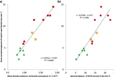
other NCFR cases previously studied (e.g., Browning and Harrold 1970;Browning and Pardoe 1973;Browning 1990), the prefrontal flow is typically orientated nearly parallel to the NCFR. Therefore, the magnitude of cross-frontal convergence will depend largely on the magnitude of the line-normal component of winds postfront. This dependency is demonstrated by the strong positive correlation (r2 5 0.90) between the mean domain-maximum convergence and the typical magni-tude of the line-normal component of wind within a 30-km-wide zone to the rear of the NCFR (Fig. 10a) (note that the latter parameter was estimated from a sequence of analyses of front-normal wind speed, us-ing the same method as for the estimation of mean pre and postfrontal wind speeds inFig. 5, as described insection 3a). Contributions to the line-normal convergence asso-ciated with prefrontal winds orientated with a component FIG. 10. Scatterplots of (a) horizontal convergence vs the NCFR-normal component of winds postfront and

of motion toward the front (e.g., as evident in some loca-tions inFigs. 4aand6a) did occasionally occur, but these were small in comparison to contributions associated with the postfrontal winds. The cross-front convergence is largest in type-ALVcases, since the near-908wind veer is associated

with postfrontal winds orientated nearly normal to the NCFR, and postfrontal wind speeds remain strong. In contrast, in type-B cases, the line-normal component of flow postfront is limited by the marked reduction in wind speeds postfront, in spite of the sometimes large wind veer. In type-ASVcases, while wind speeds remain strong postfront, the

smaller wind veer is associated with a smaller line-normal component of flow. The smaller cross-frontal convergence in type-ASVand -B cases may be a limiting factor for the

development of very narrow (and potentially barotropically unstable) zones of extremely strong shear, such as were observed in some of the type-ALVevents, as will be shown

below.

A strong positive correlation also exists between the rate of advance of the NCFR in the direction normal to its length and the line-normal component of the post-frontal winds (Fig. 10b). In a NCFR-relative reference frame, inflow of prefrontal air is strongest in the faster-moving NCFRs, given the typically near-line-parallel prefrontal flow direction. The relationship between strong cross-frontal convergence (and associated stron-ger stretching), strong line-normal postfrontal winds, rapid normal forward motion, and strong line-relative inflow could help to explain the higher tor-nado probabilities in NCFRs with large (.15 m s21) line normal forward motions, as found in a 2003–10 clima-tology of linear convective systems in the United King-dom (Clark 2013).

4. Detailed analysis of two cases: 23 December 2011 and 3 January 2012

For the NCFRs of 23 December 2011 and 3 January 2012, surface temperature, wind and pressure were fur-ther analyzed to investigate the large stretching in-creases. Radar reflectivity and radial wind data were also analyzed to investigate the smaller-scale (i.e., misoscale to small mesoscale) structure of the NCFR and its evolution in the regions of large, and increasing, vorticity stretching. On 23 December 2011, the wind and pressure fields exhibited type-B structure at the begin-ning of the analysis period (0900 UTC), with generally light winds immediately to the rear of the front. The NCFR at this time was relatively weak (rainfall rates generally,8 mm h21) and occurred only intermittently along the length of the cold front. From around 1000 UTC, postfrontal winds began to increase with a number of discrete wind maxima evident by 1100 UTC

(labeled ‘‘A,’’ ‘‘B,’’ and ‘‘C’’ inFigs. 11a–c). The general increase in winds behind the front appears to be related to the northeastward movement along the front of a subtle frontal wave (the wave is evident as an inflection point in the front over North Wales inFig. 1l), though the exact locations of individual wind maxima appear to correspond to areas where the land track is smaller be-hind the front, in the direction of the postfrontal flow (investigation of the latter aspect is outside the scope of the present study, but may warrant further inves-tigation). South of the wave apex, contraction in the cross-front direction is suggested by the increase in cross-frontal temperature gradients and narrowing of the frontal shear zone, and the NCFR began to intensify. The initial sharp increase in stretching between minutes 300 and 360 (Fig. 9a) was associated with the de-velopment of postfrontal wind maxima A and B over Wales. The second sharp stretching increase between minutes 370 and 390 (1310–1330 UTC) appears to be related to postfrontal wind speed maximum C, which developed over the Somerset area between 1200 and 1300 UTC (Figs. 11c,d). Radar data show that the line segment located at the leading edge of this wind maxi-mum bulged forward considerably between 1300 and 1330 UTC (cf. Figs. 12a,c). It was along this bulging segment that a small tornado occurred at;1410 UTC.

The bulging line segment was sampled at close range by a C-band (5.3-cm wavelength) Doppler radar located at Wardon Hill, Dorset (Fig. 12). At the time of the event, the radar was undertaking high-resolution (75-m range resolution, 18beamwidth) azimuthal scans of re-flectivity and radial winds. The tornado occurred only 9.4 km east-southeast of the radar. The line of wind veer (and associated cyclonic shear) along the NCFR is highlighted by the abrupt change in radial veloci-ties (best seen at 1311 and 1331 UTC;Figs. 12b,c). At 1251 UTC, immediately prior to the bulging, a channel of strong winds is evident immediately behind the line segment (labeled with an arrow inFig. 12a), consistent with the location of the observed maximum in surface winds over Somerset (Fig. 11c). Since the radar beam was orientated approximately normal to the NCFR in this region, a line-relative rear inflow of;5–8 m s21

can be inferred from the radial winds of 20–23 m s21

the apex of the bulge and moved gradually to the north of the apex before weakening (Fig. 13). The spacing of vortices along the line was fairly regular. For vortices forming as a result of HSI, theory predicts that the spacing of vortices should be;7.5 times the width of the shear zone (Miles and Howard 1964). Given an ob-served shear zone width of 0.6260.27 km near the apex of the bulging segment, a vortex spacing of 4.762.0 km would be expected, which is in good agreement with the mean observed vortex spacing of 5.13 km (standard de-viation of 1.68 km).

The observed increases in vorticity and vorticity stretching in the 3 January 2012 case can similarly be

linked to changes in the wind speed and direction im-mediately to the rear of the NCFR. Again, these changes apparently occurred in association with a low-amplitude wave which moved east-northeast along the front. The wave is not evident in surface analysis charts (Fig. 1f). However, in composite radar imagery (Fig. 14), its apex is marked by a subtle but persistent inflection point in the line (marked by a ‘‘W’’ in Fig. 14), which moved northeast along the front between 1000 and 1200 UTC. To the northeast of the wave apex, the pressure and wind fields generally exhibited a type-ASVconfiguration

(Fig. 15a), with strong pre- and postfrontal winds but relatively small cross-frontal veering (generally#458). FIG. 11. Wind and temperature fields at (a) 1150, (b) 1220, (c) 1350, and (d) 1430 UTC 23 Dec 2011. Wind speeds

However, immediately to the southwest of the wave apex, postfrontal winds increased slightly in speed, and veered from westerly to northwesterly between 1000 and 1200 UTC (cf. Figs. 15a,c). At the same time, a postfrontal pressure surge developed, such that the wind and pressure fields here were of type-ALV

config-uration by ;1100 UTC. The relatively strong, veered winds were restricted to a narrow strip immediately behind the front, no more than 20–30 km wide.

A sequence of vorticity stretching over southern En-gland highlights the associated development of large stretching values along the NCFR southwest of the wave apex between 1000 and 1200 UTC (Fig. 16). The largest values developed over central-southern England around 1100 UTC, and then progressed east-northeast through the London area and into parts of East Anglia. Most of the tornadoes occurred within this corridor of large stretching values.

Sequences of radar data show a fracturing of the NCFR to the southwest of the wave apex into a number of line segments and gaps between 1100 and 1300 UTC (cf.Figs. 14b,d). A closer view of the fracturing pro-cess along part of the NCFR is provided by the Chenies, Buckinghamshire, Doppler radar. At 1113 UTC, the wave apex was located;30 km west of the radar (note the associated line gap and overlapping line segments in

1240 UTC (not shown), the gaps associated with each vortex had merged leaving a larger gap of width;12 km in the along-line direction.

The localized perturbations in the line to the east and northeast of the radar at 1208 UTC (marked as C and D inFig. 17c) suggest the presence of other, smaller vor-tices elsewhere along the NCFR, but resolution limita-tions and noise in the velocity data prevent their positive identification. Vortex C was associated with a short-lived tornado near Hainault at;1200 UTC, while vortex D produced a suspected tornado at Great Waltham at approximately the same time. The other reported tor-nadoes in this case occurred out of range of the Doppler radar. As on 23 December 2011, no anticyclonic vortices were observed, but confidence that none occurred is lower than on 23 December 2012 owing to the lower resolution of the available Doppler radar data.

In summary, the detailed analysis of these two cases has shown that vorticity stretching increases along the NCFR were associated with a veering and/or increase in speed of the postfrontal winds. Doppler radar data show that, near these evolving postfrontal wind features, the NCFR vortex sheet became narrow, intense, and prone to misocyclone development. The occurrence, within 20–30 min, of five tornadoes at widely spread points along the NCFR in the 3 January 2012 case suggests that increases in vorticity and the associated miso-vortexgenesis occurred nearly simultaneously along

a section of the line at least 200 km in length. Therefore, a link is evident between the evolution of the postfrontal wind field and associated increases in cross-line vertical vorticity on the mesoscale and the genesis of vortices (and genesis of tornadoes in association with some of those vortices) on the misoscale.

The observations provide some limited evidence that HSI may have been responsible for the development of misocyclones and their associated tornadoes in these cases. For example, single-signed, cyclonic vortices were observed in both cases, with a regularly spaced line of cyclonic vortices generated in the 23 December 2011 case. The apparent absence of anticyclonic vortices in both cases is suggestive of HSI, since the alternative genesis mechanism of horizontal vortex tilting by lo-calized updrafts or downdrafts on the line would result in cyclonic–anticyclonic vortex pairs, at least in the ini-tial phase of development (Trapp and Weisman 2003). The lack of variability in reflectivity on the misoscale within line segments exhibiting misocyclone develop-ment (e.g.,Fig. 12) suggests an absence of well-marked, localized updraft and downdraft maxima on this scale, which would be required for the generation of misoscale vortices by the tilting of horizontal vorticity, either as-sociated with the ambient vertical wind shear or with density gradients across the leading edge of the line.

Nevertheless, the occurrence of the tilting mechanism cannot be ruled out given the observations available. FIG. 13. Vortex tracks (bold lines) and location of wind shear line associated with NCFR at

The vertical wind shear in the prefrontal environments of most tornadic NCFRs was within the range of values known to support strong leading line vortices in mod-eled quasi-linear convective systems [e.g.,Weisman and Trapp (2003); i.e., 0–2.5-km above ground level shear exceeding 20 m s21; see Table 1]. However, the shear magnitude also exceeded 20 m s21 in half of the non-tornadic cases, and no significant difference in mean shear magnitude was found between the tornadic and nontornadic NCFRs. It is plausible that on the meso-scale, the tilting of horizontal vorticity by differential vertical motions along the line could modulate the magnitude of vertical vorticity. If updrafts were maxi-mized near the apex of mesoscale bulges along the line, as suggested by the generally larger values of horizontal convergence near mesoscale line bulges, tilting of baro-clinic horizontal vorticity would act to increase (de-crease) vertical vorticity north (south) of the bulge apex. Another possibility, as suggested by the presence of lo-cal minima in the postfrontal temperature fields in some cases (e.g.,Fig. 15c), is that the magnitude of baroclinic horizontal vorticity is variable along the line. The rela-tive magnitude of the baroclinic horizontal vorticity and the horizontal vorticity associated with the vertical wind shear influences the angle and depth of updrafts at the leading edge of the line (e.g.,Weisman 1993); deeper

and more vertical updrafts result when the vorticity as-sociated with each is approximately balanced, increasing the magnitude of vertical vortex stretching (e.g.,Weisman and Trapp 2003). In cases where the NCFR updrafts are generally forward sloping, as might be associated, for example, with strong vertical shear in the direction normal to the line, an enhanced cold pool could act to increase the verticality of frontal updrafts.

In the absence of direct observations, or of short-range, high-resolution model predictions of vertical motions in the studied cases, the relative importance of these and other possible vortexgenesis mechanisms cannot be explored. Idealized simulations of NCFRs, in which postfrontal winds are systematically adjusted on different spatiotemporal scales, or real-data simulations in which the mesoscale bulges in the NCFR are evident in the model data, could provide insight.

The bulging configuration of the tornadic line segment on 23 December 2011, and of the NCFR southwest of the wave apex on 3 January 2012, suggest a subtle ac-celeration of the line on the mesoscale in each case. This acceleration may be related to the development of stronger line-normal, postfrontal winds near these sec-tions of NCFR, associated with the evolving postfrontal wind features previously described (e.g., recall the strong relationship found between the line-normal, postfrontal FIG. 14. Composite rainfall radar imagery for (a) 1000, (b) 1100, (c) 1200, and (d) 1300 UTC 3 Jan 2012. The W

FIG. 15. Surface temperature (shaded) and wind vectors for (a) 1000, (b) 1055, and (c) 1150 UTC 3 Jan 2012. Solid blue contours show wind speed (contours at 2 m s21 in-tervals for wind speeds$17 m s21

winds and the overall rate of advance of the front in the direction normal to its length;Fig. 10b). These features are reminiscent of the bulges that sometimes form along the leading edge of quasi-linear convective systems, such as the individual bulges that comprise a line echo wave pattern (Nolen 1959), or bow echoes that are embedded within larger-scale quasi-linear convective systems (e.g.,

Przybylinski and DeCaire 1985; Johns and Hirt 1987;

Klimowski et al. 2004). In the analyzed cases, the resulting change in line-normal forward motion was generally only a small fraction of the total line-normal forward motion. However, in extreme cases, the time-compositing analysis could break down if the local system motion vector de-viates substantially from the mean system motion vector. In the two cases analyzed in detail, the observed changes in postfrontal winds and the associated vorticity and stretching increases appeared to be related to the development, or movement along the front, of subtle frontal waves. An open question is whether the waves are a consequence of dynamical processes internal to the frontal rainband, or of external factors, such as a re-sponse of the wind field to dynamic forcing in the vicinity of the NCFR (e.g., Browning and Reynolds 1994;

Browning et al. 1997). Evaporative cooling in the wide cold frontal rainband (e.g.,Matejka et al. 1980;Ferris 1989; Browning 1990), is one mechanism by which stronger postfrontal winds could develop; locally en-hanced cooling and associated descent could increase low-level divergence behind the line, thereby increasing rear inflow in the zone between the region of maximum divergence and the NCFR. The existence of a stronger pressure surge behind the NCFR in the type-ALVcases

(Table 1) would be consistent with the idea of stronger evaporative cooling in these cases than for type-B events, since hydrostatic pressure increases would be expected where cooling occurs, and possibly even non-hydrostatic pressure increases, as described byMarsham et al. (2010). The mean value, over the seven type-ALV

cases analyzed, of the largest observed pressure increase over a line-normal distance of 10 km postfront was 2.61 hPa. This compares to 1.11 hPa for the type-B cases (values for individual cases are given inTable 1). Attest showed the difference in maximum-observed 10-km pressure increase between type-ALV and type-B cases

to be significant at the 99% level.

5. Role of stability and horizontal shear

Of the tornadic NCFRs analyzed, those of 29 August and 12 September 2012 were unusual in that they exhibited comparatively small vorticity and vorticity stretching. Given that these events occurred in late summer, it is feasible that the environmental static sta-bility was lower than in many of the late autumn and winter NCFRs. Moore (1985) describes a theoretical model of the instability of NCFRs, dependent on the static stability in the rainband, its vorticity, and other parameters such as the aspect ratio of depth to cross-frontal width.Moore (1985) found that in general, in-stabilities can have the characteristics of convective (‘‘gravity’’) modes, dominated by vertical circulations and the potential energy of the basic state, or the characteristics of sheared (‘‘shear gravity’’) modes, dominated by the horizontal motion and the kinetic energy of the shear zone. FIG. 16. Vorticity stretching (.0.0131025_s22_{shaded) at 20-min intervals between 0700 and}

The sheared mode therefore naturally represents an ex-tension of the pure ‘‘HSI’’ model to a convecting system. The sheared mode in particular tends to be stabilized when the frontal zone has a shallow aspect ratio: in interpreting our results in relation toMoore’s (1985)theoretical model, we can note that horizontal convergence and vertical stretching will lead to a deeper aspect ratio of the frontal zone, favoring the sheared mode of frontal instability, and will tend to increase the available kinetic energy for

sheared modes. Indeed, Doppler radar data suggested an aspect ratio of.1, locally, along the shear zone in the 23 December 2012 NCFR. For a given aspect ratio,Moore (1985)characterized the solutions according to the ratio of the vorticity of the shear zonejto the saturated Brunt– Väisälä FrequencyNsin the shear zone, finding that the

sheared mode existed for high ratios ofj/Ns.

An estimate ofNsfor each of the 15 analyzed NCFRs

was obtained from representative radiosonde data FIG. 17. (a)–(c) Sequence of (left) radial velocity and (right) reflectivity images from the

(assessed as those that sampled the pre-NCFR envi-ronment and were within 300 km of the NCFR at the time of the sounding; the mean distance ahead of the NCFR was 90 km). The soundings were modified using observed surface temperatures immediately ahead of the line, and the meanN2

s in the 0–1-km layer was

esti-mated using the following equation:

N2_s5 g

u_(z

0)

" u_e(z

0)2ues(z1) h_(z

0)2h(z1)

#

, (1)

whereueis the equivalent potential temperature,uesis

the saturated equivalent potential temperature, andhis the geometric height. Subscriptsz0andz1denote values

at the lower and upper bounds of the 0–1-km layer, andN2

s can take both positive and negative values. The

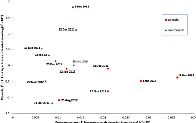
29 August 2012 NCFR was associated with lower satu-rated static stability than in all but one of the analyzed cases, but on 12 September 2012 the stability was close to the mean value for all cases (Fig. 18). In general, however, it may be inferred from Fig. 18 that tornadoes occur when the ratio ofj/Nsis relatively high. Tornadic lines all

exhibited potential instability in the 0–1-km layer (neg-ative values ofNs2), suggesting that potential instability

may be a requirement for tornadogenesis. The occur-rence of nontornadic lines in unstable conditions with low j, however, suggests that the vorticity must also be above some threshold value for tornadogenesis to occur.

6. Conclusions

Application of a time-compositing technique to 1-min-resolution surface data and interpolation onto a

5-km grid has yielded surface analyses capable of re-solving much of the small-mesoscale structure in sur-face parameter fields near to NCFRs, in addition to some;kilometer-scale features in the cross-front di-rection. Although NCFRs were all associated with strong gradients in the wind and temperature fields, large differences were evident in the post-NCFR pre-ssure and wind fields from case to case. In contrast, the pre-NCFR wind fields exhibited less variability, with the flow typically orientated nearly parallel to (within

;208of) the NCFR, in agreement with previous stud-ies. Three basic configurations of the wind field were identified (though a spectrum of types likely exists). At scales resolvable by the analyses, the magnitude of vorticity, convergence, and vorticity stretching along the NCFR, and the associated potential for misocy-clone genesis and tornadogenesis, appear to be con-trolled primarily by the configuration of the postfrontal flow. In summary:

d Large values of convergence, vorticity, and vorticity

stretching only occurred where wind speeds were strong in both the pre- and postfront environment and the cross-frontal wind veer was large (optimally near 908) (i.e., type ALVNCFRs). Tornadoes occurred

in all seven such cases analyzed.

d Smaller values of vorticity and vorticity stretching

occurred where the wind veer was small (,;408–508), or the winds fell light immediately postfront (type ASV

and B cases, respectively). Such events were appar-ently not conducive to tornado occurrence.

d NCFRs that produced several tornadoes generally

exhibited a well-defined period of increasing vorticity FIG. 18. Scatterplot of mean 0–1 kmN2

svsj 2

stretching, with the tornadoes occurring near the time of maximum vorticity stretching.

d Increases in vorticity stretching were found to be

associated with a progressive veering of winds and/or an increase in wind speed immediately behind meso-scale sections of the NCFR (i.e., an evolution in the wind field from types ASVor B to type ALV).

d In two such cases, misocyclones were observed to

develop along the frontal shear zone during the latter stages of vorticity-stretching increase, some of which were collocated with the recorded locations of the tornadoes.

d All seven tornadic NCFRs exhibited conditional

in-stability in the prefrontal environment (negativeNs2),

suggesting that this may be a necessary condition for tornadogenesis. Moreover, the two cases of condi-tional instability that did not produce a tornado both exhibited small vertical vorticity. Analysis of a greater number of cases would be needed to more clearly establish whether a functional relationship controlled by j/Ns (Moore 1985) can act as a criterion for

tornadogenesis.

Although a detailed investigation of the processes leading to changes in postfrontal winds is beyond the scope of this paper, the results suggest that the de-velopment and movement along the front of frontal waves may be involved. Further research is required to identify the relevant dynamical processes leading to such changes. Another open question to be addressed by future research is whether the type of wind and pressure field near the NCFR has any relation to the parent cy-clone type, distance from the parent cycy-clone center, or to the developmental stage of the parent cyclone.

Finally, the results of this study indicate that there is great potential in the use of the 1-min automatic weather station data, in a time-compositing analysis technique, to analyze atmospheric fields over the United Kingdom at the 5-km scale for weather systems that have relatively slow system-relative evolution. Future work should consider automation of the procedure, including opti-mization of the system propagation vector and in-terpolation scales, and the possible use of more sophisticated ‘‘time-to-space’’ analysis schemes such as the Barnes’s scheme (Barnes 1994a).

Acknowledgments.We wish to thank the anonymous reviewers whose comments have improved the pre-sentation and content of this paper. Doug Parker was supported by the DIAMET project, funded by the Nat-ural Environment Research Council (NE/I005218/1). Some of the analysis was conducted while Matt Clark was on a secondment to the University of Leeds.

REFERENCES

Atkins, N. T., R. M. Wakimoto, and T. M. Weckwerth, 1995: Ob-servations of the sea-breeze front during CaPE. Part II: Dual-Doppler and aircraft analysis.Mon. Wea. Rev.,123,944–969, doi:10.1175/1520-0493(1995)123,0944:OOTSBF.2.0.CO;2. Barnes, S. L., 1994a: Applications of the Barnes objective analysis

scheme. Part I: Effects of undersampling, wave position, and station randomness.J. Atmos. Oceanic Technol.,11,1433–1448, doi:10.1175/1520-0426(1994)011,1433:AOTBOA.2.0.CO;2. ——, 1994b: Applications of the Barnes objective analysis scheme.

Part II: Improving derivative estimates. J. Atmos. Oceanic Technol.,11,1449–1458, doi:10.1175/1520-0426(1994)011,1449: AOTBOA.2.0.CO;2.

Bishop, C. H., and A. J. Thorpe, 1994: Frontal wave stability during moist deformation frontogenesis. Part II: The suppression of nonlinear wave development. J. Atmos. Sci., 51, 874–888, doi:10.1175/1520-0469(1994)051,0874:FWSDMD.2.0.CO;2. Brown, M. J., J. D. Locatelli, M. T. Stoelinga, and P. V. Hobbs, 1999: Numerical modelling of precipitation cores on cold fronts.J. At-mos. Sci.,56,1175–1196, doi:10.1175/1520-0469(1999)056,1175: NMOPCO.2.0.CO;2.

Browning, K. A., 1990: Organization of clouds and precipitation in extratropical cyclones. Extratropical Cyclones: The Erik Palmén Memorial Volume,C. Newton and E. O. Holopainen, Eds., Amer. Meteor. Soc., 129–153.

——, 1995: On the nature of the mesoscale circulations at a kata-cold front.Tellus,47A,911–919, doi:10.1034/j.1600-0870.1995.00128.x. ——, 2004: The sting at the end of the tail: Damaging winds asso-ciated with extratropical cyclones.Quart. J. Roy. Meteor. Soc.,

130,375–399, doi:10.1256/qj.02.143.

——, and T. W. Harrold, 1970: Air motion and precipitation growth at a cold front.Quart. J. Roy. Meteor. Soc.,96,369–389, doi:10.1002/qj.49709640903.

——, and C. W. Pardoe, 1973: Structure of low-level jet streams ahead of mid-latitude cold fronts.Quart. J. Roy. Meteor. Soc.,

99,619–638, doi:10.1002/qj.49709942204.

——, and G. A. Monk, 1982: A simple model for the synoptic analysis of cold fronts.Quart. J. Roy. Meteor. Soc.,108,435– 452, doi:10.1002/qj.49710845609.

——, and F. F. Hill, 1984: Structure and evolution of a mesoscale convective system near the British Isles.Quart. J. Roy. Meteor. Soc.,110,897–913, doi:10.1002/qj.49711046607.

——, and R. Reynolds, 1994: Diagnostic study of a narrow cold-frontal rainband and severe winds associated with a strato-spheric intrusion.Quart. J. Roy. Meteor. Soc.,120,235–257, doi:10.1002/qj.49712051602.

——, N. M. Roberts, and A. J. Illingworth, 1997: Mesoscale anal-ysis of the activation of a cold front during cyclogenesis.Quart. J. Roy. Meteor. Soc.,123,2349–2375, doi:10.1002/qj.49712354410. ——, D. Jerrett, J. Nash, T. Oakley, and N. M. Roberts, 1998: Cold frontal structure derived from radar wind profilers.Meteor. Appl.,5,67–74, doi:10.1017/S1350482798000784.

Carbone, R. E., 1982: A severe frontal rainband. Part I: Stormwide hydrodynamic structure.J. Atmos. Sci.,39,258–279, doi:10.1175/ 1520-0469(1982)039,0258:ASFRPI.2.0.CO;2.

——, 1983: A severe frontal rainband. Part II: Tornado parent vortex circulation.J. Atmos. Sci.,40,2639–2654, doi:10.1175/ 1520-0469(1983)040,2639:ASFRPI.2.0.CO;2.