A L
A
TEX Package for CSLI
Collections
Edie Tor and Ed Itor (eds.)
June 29, 2001
CENTER FOR THE STUDY OF LANGUAGE
Contents
1 Efficient parsing of DOP with PCFG-reductions –
DRAFT 1
Joshua Goodman
References 21
1
Efficient parsing of DOP with
PCFG-reductions – DRAFT
Joshua Goodman
Joshua Goodman Microsoft Research One Microsoft Way Redmond, WA 98052
http://www.research.microsoft.com/˜joshuago
1.1 Introduction
While the Data-Oriented Parsing (DOP) approach has produced some extremely interesting and promising results (Bod 2000a, Bod 2000c, Bod 2000b, Bod 2001), its computational complexity has deterred its wider use, and made experiments with it more difficult. In particular, in its original form, sometimes called DOP-1 (Bod 1995a), the DOP model calls for using all possible subtrees in a training corpus. This leads to exponentially many trees, and thus both exponential time and space requirements. On top of this, the typical optimization criterion, most probable parse, is NP-complete to solve for, leading to an exponentially hard problem of exponential size. The solution has typically been various approximations, such as sampling from the set of all trees, to reduce the size of the grammar, or sampling from the set of all parses – Monte Carlo approximations – to reduce the difficulty of the search. In this chapter, we present two alternate solutions. The first removes the exponentiality of the grammar size, making it instead linear in the training data size,
1
A LATEX Package for CSLI Collections.
Edie Tor and Ed Itor (eds.).
while producing an identical distribution over parse trees. The second removes the exponentiality of the search, making it instead O(n3), by
changing slightly the search criterion, to one which is much easier, but gives almost identical performance. Our two new techniques can be used either separately, or together. Overall, together these techniques lead to a 500 times speedup over conventional DOP parsing.
1.1.1 Overview
In Section 1.2 we will show how to build a Probabilistic Context Free Grammar (PCFG) equivalent to the classic DOP model. Our model will only be linear in the size of each training tree, instead of the classic use of all possible subtrees, which produces a grammar that is typically exponential in the size of each training tree. Despite this drastically smaller size, we prove that the two models produce the same probabil-ity distributions over parse trees. This can lead to substantially faster parsing times. The grammars produced can be used with most of the typical parsing algorithms used for DOP, including an n-best parser; a monte-carlo parser; or the new parser introduced in this chapter.
We then continue more speculatively, showing variations on this ef-ficient PCFG construction that have other desirable properties. For in-stance, we can build models that limit subtree depth, or that give a smaller weight to larger trees, or that give the same weight to each piece of training data, or that when parsed, return the shortest derivation. Our construction makes it easy to do a wide variety of experiments.
Next, we describe a different maximization criterion. The usual max-imization criterion for DOP models is the most probable parse criterion, which selects the parse tree that has the highest probability of producing the sentence. However, finding the most probable parse is NP-hard. In-stead, we argue for finding the maximum constituents parse, which can be done in O(n3) time. Theoretically, the maximum constituents parse
S
!!!"""
NP
!! ""
pn pn
VP
!! ""
V NP
!!""
det n
FIGURE1 Training corpus tree for DOP example
1.1.2 The DOP-1 model
The DOP-1 model (Bod 1995a) was the first version of DOP, and most other versions of DOP are variations on it. We thus concentrate on that model. The model itself is extremely simple and can be described as follows: for every sentence in a parsed training corpus, extract every subtree. In general, the number of subtrees will be very large, typically exponential in sentence length. Now, use these trees to form a Stochastic Tree Substitution Grammar (STSG). Each tree is assigned a number of counts, one count for each time it occurred as a subtree of a tree in the training corpus. Each tree is then assigned a probability by dividing its number of counts by the total number of counts of trees with the same root nonterminal.
Given the tree of Figure 1, we can use the DOP model to convert it into the STSG of Figure 2. The numbers in parentheses represent the probabilities. To give one example, the tree
NP
!!""
det n
is assigned probability 0.5 because the tree occurs once in the training corpus, and there are two subtrees in the training corpus that are rooted in NP, so 1
2 = 0.5. The resulting STSG can be used for parsing.
In theory, the DOP model has several advantages over other models. In the conventional use of PCFGs (although not the use shown in this chapter), only a very small context is captured – perhaps a parent and its children. DOP’s use of trees allows capturing large contexts, making the model more sensitive. Since every subtree is included, even trivial ones corresponding to rules in a conventional PCFG, novel sentences with unseen contexts may still be parsed.
NP (12)
!!""
det n
VP (12)
!! ""
V NP
VP (12)
!! ""
V NP
!!""
det n
NP (12)
!! ""
pn pn
S (16)
!! ""
NP VP
S (16)
!! ""
NP VP
!! ""
V NP
S (16)
!!! """
NP VP
!! ""
V NP
!!""
det n
S (16)
!! ""
NP
!! ""
pn pn
VP
S (16)
!!!"""
NP
!! ""
pn pn
VP
!! ""
V NP
S (16)
!!!"""
NP
!! ""
pn pn
VP
!! ""
V NP
!!""
det n
FIGURE2 Sample STSG Produced from DOP Model
1.1.3 Different Criteria
Before our research, there were two existing ways to parse using the DOP model. First, one can find the most probable derivation. That is, there can be many ways a given sentence could be derived from an STSG. Using the most probable derivation criterion, one simply finds the most probable way that a sentence could be produced. Figure 3 shows a simple example STSG. For the stringxx, what is the most probable derivation? The parse tree
S ! !"" A x C x
has probability 3
9 of being generated by the trivial derivation containing
a single tree. This tree corresponds to the most probable derivation of xx.
S (39) ! !"" A x C x
S (29)
! !"" A x D x
S (29)
! !"" E x B x
S (29)
! !"" E x B B (1) x
FIGURE3 Simple Example STSG
S ! !"" E x B x each with probability 2
9, so that the parse tree has probability 49. This
parse tree is most probable.
Bod (1993b) shows how to approximate this most probable parse us-ing a Monte Carlo algorithm. The algorithm randomly samples possible derivations, then finds the tree with the most sampled derivations. Bod shows that the most probable parse yields better performance than the most probable derivation on the exact match criterion.
Sima’an (1996b, 1999) has discussed other ways of speeding up DOP parsing, mostly by limiting the sets of trees used, such as by limiting the number of substitution sites for the trees. Sima’an (1996a) shows that computing the most probable parse of a STSG is NP-Complete.
In Section 1.3 we will discuss a different way to speed up DOP pars-ing. We will show that there is a third criterion, in addition to the most probable parse and the most probable derivation, that can be used for parsing. In particular, we will find the parse with the largest number of expected correct parts: the maximum constituents parse. This criterion turns out to be much faster to maximize than the most probable parse: it can be found in timeO(n3), instead of being NP-complete. As we will
show, when tested on the ATIS corpus, it performs just as well. corpus.
1.2 Equivalent Grammar
1.2.1 PCFG for DOP-1
S@1
!!!"""
NP@2
!! ""
pn pn
VP@3
!! ""
v NP@4
!!""
det n
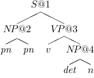
FIGURE4 Example tree with addresses
generates the same trees with the same probabilities, although one must sum over several PCFG trees for each STSG tree.
To show this reduction and equivalence, we must first define some terminology. We assign every node in every tree a unique number, which we will call its address. LetA@kdenote the node at addressk, whereA is the non-terminal labeling that node. Figure 4 shows the example tree augmented with addresses. We will need to create one new non-terminal for each node in the training data. We will call this non-terminal Ak.
We will call non-terminals of this form “interior” non-terminals, and the original non-terminals in the parse trees “exterior.”
Let aj represent the number of nontrivial subtrees headed by the
nodeA@j. Letarepresent the number of nontrivial subtrees headed by nodes with non-terminalA, that isa=!jaj.
Consider a nodeA@j of the form: A@j
!! ""
B@k C@l
How many nontrivial subtrees does it have? Consider first the possibili-ties on the left branch. There arebk non-trivial subtrees headed byB@k,
and there is also the trivial case where the left node is simplyB. Thus there are bk+ 1 different possibilities on the left branch. Similarly, for
the right branch there arecl+1 possibilities. We can create a subtree by
choosing any possible left subtree and any possible right subtree. Thus, there areaj = (bk+ 1)(cl+ 1) possible subtrees headed byA@j. In our
example tree of Figure 4, both noun phrases have exactly one subtree: np4=np2= 1; the verb phrase has 2 subtrees:vp3= 2; and the sentence
has 6:s1 = 6. These numbers correspond to the number of subtrees in
Figure 2.
[image:9.612.249.343.139.217.2]S
!!!"""
N P
!! ""
P N P N
V P
!! ""
V NP
S (external)
!!!"""
N P@1
!! ""
P N P N
V P@2 (internal)
!! ""
V N P (external)
STSG elementary homomorphic PCFG
tree subderivation
FIGURE5 STSG elementary tree homomorphic to a PCFG subderivation
taken from Figure 2, and a homomorphic PCFG subderivation.
We will give a simple small PCFG with the following surprising prop-erty: for every subtree in the training corpus headed by A, the gram-mar will generate a homomorphic subderivation with probability 1/a. In other words, rather than using the large, explicit STSG, we can use this small PCFG that generates homomorphic derivations, with identical probabilities.
The construction is as follows. For a node such as A@j
!! ""
B@k C@l
we will generate the following eight PCFG rules, where the number in parentheses following a rule is its probability.
Aj →BC (1/aj) A→BC (1/a)
Aj →BkC (bk/aj) A→BkC (bk/a)
Aj →BCl (cl/aj) A→BCl (cl/a)
Aj →BkCl (bkcl/aj) A→BkCl (bkcl/a)
(1.1)
Theorem 1 Subderivations headed byAwith external non-terminals at
the roots and leaves and internal non-terminals elsewhere have probabil-ity1/a. Subderivations headed byAjwith external non-terminals only at the leaves and internal non-terminals elsewhere, have probability1/aj. Proof The proof is by induction on the depth of the trees. For trees of depth 1, there are two cases:
A
!! ""
B C
A@j
!! ""
B C
Trivially, these trees have the required probabilities.
PCFG derivation 4 productions
S
!!!!""""
N P@3
!! ""
P N P N
V P@1
!!! """
V N P
!! ""
DET N
STSG derivation 2 subtrees
S
!!!!""""
N P
!! ""
P N P N
V P
!!! """
V N P
N P
!! ""
DET N
FIGURE6 Example of Homomorphic Derivation
for each of the eight rules. We show two of them. Let B@... represent ak
tree of at most depthnwith external leaves, headed byB@k, and with internal intermediate non-terminals. Then, for trees such as
A@j
!! ""
B@k ... C@l... the probability of the tree is 1
bk 1
cl
bkcl
aj = 1
aj. Similarly, for another case,
trees headed by
A
!! ""
B@k C the probability of the tree is 1
bk
bk
a =a1. The other six cases follow trivially
with similar reasoning. !
We call a PCFG derivation homomorphic to a STSG derivation if for every substitution in the STSG there is a corresponding subderivation in the PCFG. Figure 6 contains an example of homomorphic derivations, using two subtrees in the STSG and four productions in the PCFG.
We call a PCFG tree homomorphic to a STSG tree if they are identi-cal when internal non-terminals are changed to external non-terminals.
Theorem 2 This construction produces PCFG trees homomorphic to the STSG trees with equal probability.
would be a homomorphic PCFG subderivation, with equal probability. Thus for every STSG derivation, there would be a homomorphic PCFG derivation, with equal probability. Thus every STSG tree would be pro-duced by the PCFG with equal probability.
However, it is extremely likely that some subtrees, especially trivial ones like
S
!! ""
N P V P will occur repeatedly.
If the STSG formalism were modified slightly, so that trees could oc-cur multiple times, then our relationship could be made one-to-one. Con-sider a modified form of the DOP model, in which the counts of subtrees which occurred multiple times in the training corpus were not merged: both identical trees would be added to the grammar. Each of these trees will have a lower probability than if their counts were merged. This would change the probabilities of the derivations; however the probabilities of parse trees would not change, since there would be correspondingly more derivations for each tree. Now, the desired one-to-one relationship holds: for every derivation in the new STSG there is a homomorphic derivation in the PCFG with equal probability. Thus, summing over all derivations of a tree in the STSG yields the same probability as summing over all the homomorphic derivations in the PCFG. Thus, every STSG tree would be produced by the PCFG with equal probability.
It follows trivially from this that no extra trees are produced by the PCFG. Since the total probability of the trees produced by the STSG is 1, and the PCFG produces these trees with the same probability, no probability is “left over” for any other trees. !
1.2.2 PCFGs for Other Versions of DOP
Most experiments in DOP have limited the subtree depth. This was originally done for efficiency, although more recent experiments (Sima’an 1999) have also shown improved accuracy. Ironically, limit-ing subtree depth uslimit-ing our model naively actually makes the grammar larger, by up to a factor of the maximum depth, but is still more efficient than the direct approach. The trick is to associate depth numbers with each new node we generate, keeping a count of how deep we are.
Assume we want to model subtrees of depth at most d. We use a variation on our previous technique. Let aej represent the number of
nontrivial subtrees headed by the nodeA@jof depth at most e. Letad
represent the number of nontrivial subtrees of depth at mostd headed by nodes with non-terminalA, that isad =!jadj.
As before, consider a nodeA@j of the form: A@j
!! ""
B@k C@l We now compute ae
j. Following similar reasoning as before, there are
bek−1 non-trivial subtrees of depth at most e−1 headed by B@k, plus the case where the left node is just B, leading to bek−1+ 1 different possibilities on the left branch. Similarly, for the right branch there are cel−1+ 1 possibilities. So,ae
j = (bek−1+ 1)(c e−1
l + 1).
The construction with limited depth trees is as follows, similar to our previous construction, but with roughlyd/2 times as many rules. For a node such as
A@j
!! ""
B@k C@l we will generate the following rules:
A→BC (1/ad)
A→Bkd−1C (bdk−1/ad)
A→BCld−1 (cdl−1/ad)
A→Bkd−1Cld−1 (bdk−1cdl−1/ad)
(1.2)
Now, for each 1≤e < dwe need the following rules: Ae
j →BC (1/aej)
Ae
j →Bke−1C (b e−1
k /aej)
Ae
j →BCle−1 (c e−1
l /aej)
Ae
j →Bke−1C e−1
l (b e−1
k c e−1
l /aej)
(1.3)
Notice that if two nodesA@j andA@khave exactly the same sub-trees of depth at most e, then the productions for Ae
j and Aek can be
merged. For large trees, this is unlikely, but when the subtree depth is limited, this may be very common. (The set of all subtrees will be the same if and only if the trees are identical down to depthe. This can be detected efficiently with a good hash table.) Also, if a tree A@j is of depthe, then for allf > e, the productionsAe
j can be merged with the
productions forAfj.
These ideas can be extended even further. Sima’an (1999, page 133) notes that a variety of techniques can be used to limit the number of subtrees used: the depth, the number of substitution sites, the number of terminals, and the number of adjacent terminals. The first three can all be easily incorporated into our reduction technique, simply by adding limits analogous to the depth limit. There is also nothing to prevent these limits from also being used in combination. We could probably also apply the last technique, limiting the number of adjacent terminals, but it would be somewhat harder to do this, and probably not worth the effort.
Bod (2000c) shows that excellent results can be gotten from using the shortest derivation – smallest number of trees in the derivation – rather than the most probable parse. We can easily emulate this crite-rion, by simply giving the rules of Equation 1.1 headed by an external nonterminal a probability of 0.5, and internal nonterminal headed rules a probability of 1. The resulting grammar will, of course, not be a PCFG since the probabilities will sum to more than 1 – it might be better to think of these as weights, rather than probabilities – but the most probable derivation using this grammar has the following property: the probability of the parse is equal to 0.5k wherekis the number of
exter-nal nontermiexter-nals used, which is exactly the number of trees that would be used in the corresponding STSG derivation. The highest probabil-ity parse will be the one corresponding to the shortest derivation. Bod (2000c) gives a moderately complex ranking technique to distinguish be-tween ties; it would be necessary to use a different ranking technique in order to use our equivalence, or to break ties after the parsing step.
For instance, Bonnemaet al. suggest using P(α) = 2−N(α)f(α)/F(α)
whereαrepresents a tree,N(α) represents the number of root non-terminals in α, f(α) represents the number of times α occurs in the training data, and F(α) represents the number of times the root non-terminal ofαoccurs in the training data.
It turns out that we can create a PCFG equivalent to this model. Setaequal to the number of times nonterminals of typeAoccur in the training data, and use
Aj →BC (1/4) A→BC (1/4a)
Aj →BkC (1/4) A→BkC (1/4a)
Aj →BCl (1/4) A→BCl (1/4a)
Aj →BkCl (1/4) A→BkCl (1/4a)
(1.4)
This grammar assigns the same probabilities to subtrees as the model of Bonnema et al. Bonnemaet al. reduce the probability of a tree by a factor of two for each non-root non-terminal it contains. This is equiv-alent to reducing the probability of a tree by a factor of four for each pair of non-terminals it contains, which is exactly what we do. Note that Bod (2001) achieves excellent results while using a sampling technique that has the effect of assigning roughly equal weight to each node in the training data and very roughly exponentially less probability for larger trees, so techniques along these lines seem very promising.
Of course, there are many variations on these techniques that could be explored. For instance, an alternative that gives equal weight to each training data node, and equal weight to each subtree is:
Aj →BC (1/aj) A→BC (1/aja)
Aj →BkC (bk/aj) A→BkC (bk/aja)
Aj →BCl (cl/aj) A→BCl (cl/aja)
Aj →BkCl (bkcl/aj) A→BkCl (bkcl/aja)
(1.5)
1.3 Parsing Algorithm
As we discussed in the introduction to this chapter, there are several dif-ferent evaluation metrics one could use for finding the best parse. The two that have been used most are the most probable derivation, which can be found using the Viterbi algorithm, and the most probable parse, which can be approximated by random sampling. However, finding the most probable parse is NP-complete, and the most probable derivation has lower accuracy. In this section, we describe a third evaluation met-ric, the maximum constituents parse, which attempts to maximize the number of correct parts of the parse. We will show that this criterion can be maximized inO(n3) time, that in theory it is better for measures
like precision and recall, and, in actual experiments on the ATIS corpus, performs at least as well as the most probable parse for precision, recall, and the exact match criteria.
Parsers are often evaluated on criteria such as precision and recall, or crossing brackets rate, that roughly count the number of correct parts of a parse tree. If our performance evaluation were based on such a measure, we would want the parse tree that was most likely to have the largest number of correct constituents. Consider this criterion and the example grammar of Figure 3. Here are the three best parses in this grammar, according to different criteria:
S ! !"" A x C x S ! !"" E x B x S ! !"" A x B x
Most Most Maximum
probable probable constituents
derivation parse parse
Probability 3
9 Probability 49 2 correct pieces
We previously analyzed the most probable derivation probability (3 9) and
the most probable parse probability (4
9). For the maximum consituents
parse, we want to know how many pieces we expect are correct. The probability that theS constituent is correct is 1.0, while the probability that the A constituent is correct is 59, and the probability that the B constituent is correct is 4
9. Thus, this tree has on average 2 constituents
criterion.
Bod (1993a, 1995a) shows that the most probable derivation does not perform nearly as well as the most probable parse for the DOP model. This is not surprising, since each parse tree can be derived by many different derivations; the most probable parse criterion takes all possible derivations into account. Similarly, the maximum constituents parse is also derived from the sum of many different derivations. Fur-thermore, although the maximum constituents parse should not do as well on the exact match criterion, it should perform even better on the percent constituents correct criterion, and presumably also work better on closely related criteria such as precision and recall. We have previ-ously performed a detailed comparison between the most likely parse, and the maximum constituents parse for PCFGs (Goodman 1996b); we showed that the two have very similar performance on a broad range of measures, with at most a 10% relative difference in error rate (i.e., a change from 10% error rate to 9% error rate.) We therefore think that it is reasonable to use a maximum constituents parser to parse the DOP model.
The parsing algorithm is a variation on the Inside-Outside algor-ithm, developed by Baker (1979) and discussed in detail by Lari and Young (1990). However, while the Inside-Outside algorithm is a grammar re-estimation algorithm, the algorithm presented here is just a parsing algorithm. It is closely related to a similar algorithm (Rabiner 1989) used for Hidden Markov Models (HMMs) for finding the most likely state at each time. However, unlike in the HMM case where the algorithm produces a simple state sequence, in the PCFG case a parse tree is produced, resulting in additional constraints.
A formal derivation of a very similar algorithm is given elsewhere (Goodman 1996b); only the intuition is given here. The algorithm can be summarized as follows. First, for each potential constituent, where a constituent is a non-terminal, a start position, and an end position, find the probability that that constituent is in the parse. After that, put the most likely constituents together to form a parse tree, using dynamic programming.
The probability that a potential constituent occurs in the correct parse tree, P(X ⇒∗ ws...wt|S ⇒∗ w1...wn), will be called g(s, t, X). In
words, it is the probability that, given the sentence w1...wn, a symbol
X generates ws...wt. We can compute this probability using elements
of the Inside-Outside algorithm. First, compute the inside probabilities, e(s, t, X) =P(X ⇒∗ ws...wt). Second, compute the outside probabilities,
for length := 2 to n
for s := 1 to n-length+1 t := s + length - 1; for all non-terminals X
sum[X] := g(s, t, X); loop over addresses k
let X := non-terminal at k;
let sum[X] := sum[X] + g(s,t,X_k); loop over non-terminals X
let max_X := arg max of sum[X] loop over r such that s <= r < t
let best_split :=
max of maxc[s,r] + maxc[r+1,t]; maxc[s,t] := sum[max_X] + best_split;
FIGURE7 Maximum Constituents Data-Oriented Parsing Algorithm
g(s, t, X):
g(s, t, X) = P(S⇒∗ w1...ws−1Xwt+1...wn)P(X ⇒∗ ws...wt)
P(S⇒∗ w1...wn)
= f(s, t, X)×e(s, t, X)/e(1, n, S)
Once the matrix g(s, t, X) is computed, a dynamic programming algorithm can be used to determine the best parse, in the sense of max-imizing the number of constituents expected correct. Figure 7 shows pseudocode for a simplified form of this algorithm.
For a grammar withg nonterminals and training data of sizeT, the run time of the algorithm is O(T n2+gn3 +n3) since there are two
layers of outer loops, each with run time at most n, and inner loops, over addresses (training data), nonterminals and n. However, this is dominated by the computation of the Inside and Outside probabilities, which takes time O(rn3), for a grammar with r rules. If we use the
construction of section 1.2, there are eight rules for every node in the training data, making the overall runtimeO(T n3).
By modifying the algorithm slightly to record the actual split used at each node, we can recover the best parse. The entry maxc[1, n]
contains the expected number of correct constituents, given the model.
1.4 Experimental Results and Discussion
ex-Criteria Min Max Mean StdDev
Cross Brack DOP 86.53% 96.06% 90.15% 2.65%
Cross Brack P&S 86.99% 94.41% 90.18% 2.59% Cross Brack DOP−P&S -3.79% 2.87% -0.03% 2.34% Zero Cross Brack DOP 60.23% 75.86% 66.11% 5.56% Zero Cross Brack P&S 54.02% 78.16% 63.94% 7.34% Zero Cross Brack DOP−P&S -5.68% 11.36% 2.17% 5.57%
TABLE1 DOP versus Pereira and Schabes on Minimally Edited ATIS
Criteria Min Max Mean StdDev
Cross Brack DOP 95.63% 98.62% 97.16% 0.93%
Cross Brack P&S 94.08% 97.87% 96.11% 1.14% Cross Brack DOP−P&S -0.16% 3.03% 1.05% 1.04% Zero Cross Brack DOP 78.67% 90.67% 86.13% 3.99% Zero Cross Brack P&S 70.67% 88.00% 79.20% 5.97% Zero Cross Brack DOP−P&S -1.33% 20.00% 6.93% 5.65%
Exact Match DOP 58.67% 68.00% 63.33% 3.22%
TABLE2 DOP versus Pereira and Schabes on Bod’s Data
Labelled Most Pereira
Recall Probable and Significant
Parse Parse Schabes
Cross Brack 90.1 90.0 90.2
0 Cross Brack 66.1 65.9 63.9
Exact Match 40.0 39.2
TABLE3 Three way comparison on minimally edited ATIS data
Labelled Most Pereira
Recall Probable and Significant
Parse Parse Schabes
Cross Brack 97.2 97.1 96.1 √
0 Cross Brack 86.1 86.1 79.2 √
Exact Match 63.3 63.1
periments (Bod 1995b, Bod 1995a, Bod 1993b). The original ATIS data from the Penn Tree Bank, version 0.5, is very noisy; it is difficult to even automatically read this data, due to inconsistencies between files. Researchers were thus left with the difficult decision as to how to clean the data. For this paper, we conducted two sets of experiments: one us-ing a minimally cleaned set of data, makus-ing our results comparable to previous results; the other using the ATIS data prepared by Bod, which contained much more significant revisions.
Ten data sets were constructed by randomly splitting minimally edit-ed ATIS (Hemphill et al., 1990) sentences into a 700 sentence training set, and 88 sentence test set, then discarding sentences of length >30. For each of the ten sets, both the DOP algorithm outlined here and the grammar induction experiment of Pereira and Schabes (1992) were run. Crossing brackets, zero crossing brackets, and the paired differences are presented in Table 1. All sentences output by the parser were made bi-nary branching (Goodman 1996a), since otherwise the crossing brackets measures are meaningless (Magerman 1994). A few sentences were not parsable; these were assigned right branching period high structure, a good heuristic (Brill 1993). Note that our comparison to Pereira and Schabes parsing is much outdated. While this was roughly state of the art at the time this work was done, much more advanced techniques have since become available (Charniak 2000).
We also ran experiments using Bod’s data, 75 sentence test sets, and no limit on sentence length. However, while Bod provided us with his data, he did not provide us with the split into test and training that he used; as before we used ten random splits. The results are disappointing, as shown in Table 2. Note that they are noticeably worse than some previously reported results on this data set; elsewhere (Goodman 1996a, Goodman 1998), we examine this discrepancy more closely and show that the previous results are probably not reproducible.
DOP does do slightly better on most measures. We performed a sta-tistical analysis using at-test on the paired differences between DOP and Pereira and Schabes performance on each run. On the minimally edited ATIS data, the differences were statistically insignificant, while on Bod’s data the differences were statistically significant beyond the 98’th per-centile. Our technique for finding statistical significance is more strenu-ous than most: we assume that since all test sentences were parsed with the same training data, all results of a single run are correlated. Thus we compare paired differences of entire runs, rather than of sentences or constituents. This makes it harder to achieve statistical significance.
between the DOP and the Pereira and Schabes algorithms. Notice that the minimum is usually negative, and the maximum is usually positive, meaning that on some tests DOP did worse than Pereira and Schabes and on some it did better. It is important to run multiple tests, especially with small test sets like these, in order to avoid misleading results.
1.5 Timing and Optimization
In this section, we examine the empirical runtime of our algorithm, con-sider the run time of Monte Carlo parsing, and describe some optimiza-tions that can be applied to a Monte Carlo parser.
It takes about 6 seconds per sentence to run our algorithm on an HP 9000/7151, versus 3.5 hours to run a Monte Carlo parser using the
STSG construction on a Sparc 21 (Bod 1995b). Factoring in that the
HP is roughly four times faster than the Sparc, the new algorithm is about 500 times faster. Of course, some of this difference may be due to differences in implementation, so this estimate is fairly rough.
We also note that the run time for Monte-Carlo parsing is still ex-ponential in the sentence length. LettingGrepresent grammar size, and " represent maximum estimation error, the Monte Carlo run time is O(Gn2"−2). The"−2parameter is important; for this algorithm to have
some reasonable chance of finding the most probable parse, the num-ber of samples must be at least inversely proportional to the conditional probability of that parse. For instance, if the maximum probability parse had probability 1/50, then we need at least 50 samples to be reasonably sure of finding that parse.
Now, we note that the conditional probability of the most probable parse tree will in general decline exponentially with sentence length. We assume that the number of ambiguities in a sentence will increase linearly with sentence length; if a five word sentence has on average one ambiguity, then a ten word sentence will have two, etc. A linear increase in ambiguity will lead to an exponential decrease in probability of the most probable parse.
Since the probability of the most probable parse decreases expo-nentially in sentence length, the number of random samples needed to find this most probable parse increases exponentially in sentence length. Thus, when using the Monte Carlo algorithm, one is left with the un-comfortable choice of exponentially decreasing the probability of finding the most probable parse, or exponentially increasing the runtime. This is a somewhat informal argument, but seems reasonable. Note that our algorithm has true runtime O(T n3), as shown previously.
for k := 1 to n for i := 0 to n-k
for chart-entry (i, i+k) do for each root-node X do
select a random subderivation of root X eliminate the other subderivations
FIGURE8 Bottom-up Sampling Algorithm for a Random Derivation
Sample(Chart_Address, Symbol) {
if Symbol is a terminal return Symbol; else
select a random Entry for Symbol at Chart_Address; let Left := Sample(Entry’s left address,
Entry’s left symbol); let Right := Sample(Entry’s right address,
Entry’s right symbol); return MakeTree(Left, Right);
}
FIGURE9 Top Down Algorithm for Sampling a Random Derivation
We present a more efficient top-down version of Monte-Carlo sam-pling that can lead to large speedups. Bod (1995b) gives the pseudocode in Figure 8 for how to sample a random derivation. This is essentially a bottom up sampling scheme. For a grammar withg non-terminals, it requires timeO(gn2).2On the other hand, a top down sampling scheme
such as Figure 9 would be faster. If we callSample((0,n), S), it finds a random entry for the root node, and then proceeds to recursively se-lect random entries for each branch. Since the sampled tree will have n−1 nodes, this algorithm isO(n). This would make Monte Carlo pars-ing significantly faster, although still not nearly as fast as a maximum constituents parser.
We mention another technique that can be used to potentially speed Monte-Carlo and n-best style parsers. The normal inside algorithm can be easily modified so that it finds only the sum of derivation probabilities
2This assumes that the selection of a random chart entry can be done in constant
consistent with a particular parse. While it is NP-complete to find the most probable parse, it is only O(nP) to find the probability of any particular parse tree, where we defineP to be the maximum number of productions consistent with a part of the tree. This means that if we are performing sampling, either Monte-Carlo or best first, we need only sample long enough to get a single instance of the most probable parse, rather than long enough to accurately estimate its probability.
1.6 Conclusion
In this paper we have described a large number of potential speedups for DOP parsing. Each of these techniques can be used either sepa-rately, or together. Combining our two favorite speedups, our grammar transformation, together with a maximum constituents parser, leads to a 500 times speedup over traditional DOP parsing. Given that the heavy resource usage of DOP is the biggest problem with the formalism, we believe our speedups will be very valuable to those implementing DOP models. Most of these techniques have not been widely used in the past. We know of no reason not to use maximum constituents parsing, and hope it will receive wide usage. The grammar transformation technique has not been widely used because prior to this publication, it was only available in the full form, rather than in the depth-limited form described in Equations 1.2 and 1.3. Hopefully, it will now be more widely used.
References
Baker, James K. 1979. Trainable Grammars for Speech Recognition. InProceedings of the Spring Conference of the Acoustical Society of America, 547–550. Boston, MA, June.
Bod, Rens. 1993a. Data-Oriented Parsing as a General Framework for Stochastic Language Processing. InParsing Natural Language, ed. K. Sikkel and A. Nijholt. The Netherlands: Twente.
Bod, Rens. 1993b. Using an annotated corpus as a stochastic grammar. InProceedings of the Sixth Conference of the European Chapter of the ACL, 37–44.
Bod, Rens. 1995a. Enriching Linguistics with Statistics: Performance Models of Natural Language. University of Amsterdam ILLC Disser-tation Series 1995-14. Amsterdam: Academische Pers.
Bod, Rens. 1995b. The Problem of Computing the Most Probable Tree in Data-Oriented Parsing and Stochastic Tree Grammars. In Pro-ceedings of the Seventh Conference of the European Chapter of the ACL. Dublin, Ireland, March.
Bod, Rens. 2000a. Combining Semantic and Syntactic Structure for Language Modeling. InProceedings ICSLP-2000.
Bod, Rens. 2000b. An Improved Parser for Data-Oriented Lexical-Functional Analysis. InProceedings ACL-2000.
Bod, Rens. 2000c. Parsing with the Shortest Derivation. InProceedings COLING-2000.
Bod, Rens. 2001. What is the Minimal Set of Fragments that Achieves Maximal Parse Accuracy. InProceedings ACL-2001.
Bonnema, R., P. Buying, and R. Scha. 1999. A new probability model for data-oriented parsing. In Proceedings of the 12th Amsterdam Colloquium.
Brill, Eric. 1993.A Corpus-Based Approach to Language Learning. Doc-toral dissertation, University of Pennsylvania.
TEX Package for CSLI Collections
Charniak, Eugene. 2000. A Maximum-Entropy-Inspired Parser. In Pro-ceedings of NAACL-2000.
Charniak, Eugene. 2001. Immediate-Head Parsing for Language Models. Available fromhttp://www.cs.brown.edu/people/ec.
Collins, Michael. 2000. Discriminative reranking for natural language parsing. InProceedings ICML-2000.
Goodman, Joshua. 1996a. Efficient Algorithms for Parsing the DOP Model. InProceedings of the Conference on Empirical Methods in Natural Language Processing, 143–152. May. Available as cmp-lg/9604008.
Goodman, Joshua. 1996b. Parsing Algorithms and Metrics. In Proceed-ings of the 34th Annual Meeting of the ACL, 177–183. Santa Cruz, CA, June. Available as cmp-lg/9605036.
Goodman, Joshua. 1998.Parsing Inside-Out. Doctoral dissertation, Har-vard University. Available as cmp-lg/9805007 and fromhttp://www. research.microsoft.com/˜joshuago/thesis.ps.
Hemphill, Charles T., John J. Godfrey, and George R. Doddington. 1990. The ATIS spoken language systems pilot corpus. InDARPA Speech and Natural Language Workshop. Hidden Valley, Pennsylvania, June. Morgan Kaufmann.
Lari, K., and S.J. Young. 1990. The Estimation of Stochastic Context-Free Grammars using the Inside-Outside Algorithm. Computer Speech and Language4:35–56.
Magerman, David. 1994. Natural Language Parsing as Statistical Pat-tern Recognition. Doctoral dissertation, Stanford University Univer-sity, February. Available as cmp-lg/9405009.
Pereira, Fernando, and Yves Schabes. 1992. Inside-Outside Reestimation from Partially Bracketed Corpora. InProceedings of the 30th Annual Meeting of the ACL, 128–135. Newark, Delaware.
Rabiner, L.R. 1989. A Tutorial on Hidden Markov Models and Selected Applications in Speech Recognition. Proceedings of the IEEE77(2). Sima’an, Khalil. 1996a. Computational Complexity of Probabilistic Dis-ambiguation by Means of Tree Grammars. InProceedings Coling-96. Available as cmp-lg/9606019.
Sima’an, Khalil. 1996b. Efficient Disambiguation by Means of Stochastic Tree Substitution Grammars. In Recent Advances in NLP 1995, ed. R. Mitkov and N. Nicolov. Current Issues in Linguistic Theory, Vol. 136. Amsterdam: John Benjamins.
Sima’an, Khalil. 1999. Learning Efficient Disambigua-tion. ILLC dissertation series, No. 02. Available from