This is a repository copy of Model validation of spatiotemporal systems using correlation function tests.
White Rose Research Online URL for this paper: http://eprints.whiterose.ac.uk/74557/
Monograph:
Pan, Y. and Billings, S.A. (2006) Model validation of spatiotemporal systems using correlation function tests. Research Report. ACSE Research Report no. 915 . Automatic Control and Systems Engineering, University of Sheffield
Reuse
Unless indicated otherwise, fulltext items are protected by copyright with all rights reserved. The copyright exception in section 29 of the Copyright, Designs and Patents Act 1988 allows the making of a single copy solely for the purpose of non-commercial research or private study within the limits of fair dealing. The publisher or other rights-holder may allow further reproduction and re-use of this version - refer to the White Rose Research Online record for this item. Where records identify the publisher as the copyright holder, users can verify any specific terms of use on the publisher’s website.
Takedown
If you consider content in White Rose Research Online to be in breach of UK law, please notify us by
Model Validation of Spatiotemporal Systems Using Correlation
Function Tests
Y. Pan, S. A. Billings
Dept. of Automatic Control and Systems Engineering,
University of Sheffield
Sheffield, S1 3JD, UK
February, 2006
Abstract
Model validation is an important and essential final step in system identification. Although model validation for nonlinear temporal systems has been extensively studied, model validation for spatiotemporal systems is still an open question. In this paper, correlation based methods, which have been successfully applied in nonlinear temporal systems are extended and enhanced to validate models of spatiotemporal systems. Examples are included to demonstrate the application of the tests.
1.
Introduction
Spatiotemporal dynamic systems have become an increasingly important research area for a large range of scientific subjects including chemistry, biology, ecology, meteorology and finance. Spatiotemporal systems have traditionally been described using nonlinear Partial Differential Equations (PDE) or in discrete time form as Lattice Dynamical Systems (LDS) or a subset of LDS called Coupled Map Lattices (CML). A CML model is defined over a d-dimensional lattice where each site evolves in time through a discrete map which describes the influence of past states and neighbouring sites. CML were initially introduced in the1980s by Kaneko (1985, 1986). The CML model is discrete in both the time and space domain but has a continuous state value. PDE’s can be finitely approximated by CML, provided that certain conditions of spatial and temporal resolution have been met. Due to the computational efficiency and richness of dynamical behaviors, the analysis and identification of CML has been studied by several authors. A fundamental feature of CML is that the local state-space variables associated to each lattice node are the same over the whole lattice. In other words, these variables represent the same set of physical quantities at each node of the given lattice. The CML model can be shown to be composed of two parts: a local term involving only the local input and output variables and a spatial coupling term which describes the interactions with the neighboring lattice sites.
The purpose of model validation is to validate the correctness of the model structure and the unbiasedness of the estimated model parameters and usually involves testing the identified model on another independent set of data. It is a final and essential stage in most system identification procedures. Model validation methods can also be used to check if an identified model is under or over fitted.
one-step-ahead prediction errors should be a random time sequence with zero mean and finite variance. The auto-correlation function (ACF) and the cross-correlation function (CCF) have been widely used in linear temporal model validation (Bohlin, 1971, 1978, Soderstrom and Stoica, 1990). It is well known that the ACF of the residuals and the CCF between the residuals and input should fall within preset confidence intervals if the identified model is correct and the residual sequence is white.
Simple auto and cross correlation tests for linear models cannot be applied directly to the model validation of nonlinear temporal systems since they cannot detect all possible missing nonlinear terms in the residuals (Billings and Voon, 1983). Model validation methods for nonlinear temporal systems based on higher order correlation tests between the input and the residuals were first introduced by Billings and Voon (1983, 1986) to detect the missing nonlinear terms in the residuals. In order to achieve more discriminatory power with less computational cost, improved correlation tests based on correlation functions between the input, output and residuals were introduced in later studies (Billings and Zhu 1994, 1995; Mao and Billings 2000).
But all these methods are for purely temporal systems and unfortunately model validation tests for spatiotemporal systems are more complex. Given a derived or identified model of a spatiotemporal system in the form of a PDE, CML or LDS, model validation tests are required to determine whether the model can adequately describe the underlying dynamics of the spatiotemporal system. The only model validation methods which are available for spatiotemporal systems are based on subjectively judging the quality of the one-step-ahead prediction errors or the model predicted output (Partilz and Merkwirth 2000, Coca and Billings 2001, 2003; Timer et al. 2000; Muller and Timmer 2002. An alternative method is to compare specific dynamical characteristics like the bifurcation diagram between the modeled system and the real system (Aguirre and Billings 1994, 1995a, 1995b, Guo and Billings 2004). But a disadvantage of the latter method is that a priori information about the dynamical characteristics of the spatiotemporal system under study must be available.
In this paper, model validation methods based on higher order correlation function tests are introduced for a wide class of spatiotemporal systems and examples are included to demonstrate the performance of the new methods. This paper is arranged as follows. Section 2 formulates the problem of model validation for spatiotemporal systems. Section 3 reviews the correlation test methods for nonlinear temporal systems, while section 4 introduces the new model validation methods for spatiotemporal systems based on a set of correlation test functions. Three numerical examples are included in section 4 to illustrate the application of the new model methods and to demonstrate how the new tests can be used to detect missing or over-fitted model terms.
2.
Problem Statement
yi(t)= f(qnyyi(t),qnuui(t),qnεεi(t),qnysmyyi(t),qnusmuui(t),qnεsmεεi(t))+εi(t) f (q y (t),q u (t),q i(t))
n i n i n l
u
y εε
=
+ fc(qnyyi(t),qnuui(t),qnεεi(t),qnysmyyi(t),qnusmuui(t),qnεsmεεi(t))+εi(t) (2-1) where, spatial invariance means that the underlying dynamics in each lattice node are the same for all lattice nodes. Here, d
I
i∈ is the spatial index of a d-dimensional space and t
is the temporal index; yi(t) andui(t) are the output and input variables respectively at lattice i and time t, and εi(t) is an independent zero mean random sequence.
n
q is a temporal backward shift operator
) ,..., ,
( 1 2 n
n
q q q
q = − − − (2-2) so that
)) (
),..., 2 ( ), 1 ( ( ) (
)) (
),..., 2 ( ), 1 ( ( ) (
)) (
),..., 2 ( ), 1 ( ( ) (
ε
ε ε
ε ε
ε t t t t n
q
n t u t
u t u t u q
n t y t
y t y t y q
i i
i i
n
u i i
i i
n
y i i
i i
n
u y
− −
− =
− −
− =
− −
− =
(2-3)
where ny, nu and nε denote the maximum temporal lags corresponding to output y , inputu and the residual sequence ε.
In (2-1), m
s is a multi-valued spatial shift operator
sm =(sp1,sp2,...,spm) (2-4) where pj∈Idis the spatial translation multi-index, such that
) ,..., ,
(
) ,..., ,
(
) ,..., ,
(
2 1
2 1
2 1
ε
εε ε ε ε
m u m y
y m y
p i p i p i i m
p i p i p i i m
p i p i p i i m
s
u u
u u s
y y
y y s
− −
−
− −
−
− −
−
= = =
(2-5)
The parametersmy,muand mε denote the maximum temporal lags corresponding to the outputyinputuand the residual sequenceε. The model f :Y×U →Y is composed of the local map fl(⋅) and the coupling map fc(⋅), which can both take the form of a very wide class of linear or nonlinear models, including polynomial or wavelet expansions. The main object of model validation is to check the goodness of fit of any given model by using model validation tests. A model validation test can be formulated as a statistical hypothesis testing problem. For instance, the identified model f is set as the hypothesisHo. Then, in the first step, a parameter-free statistic is formed, which is a statistical function of the available data. Therefore, the distribution of the statistic variable is known if the hypothesis Hois true. In this paper, the residual sequence or the
one-step-ahead prediction error εi(t) associated with model (2-1) is used as a statistic variable. So if the hypothesis Ho for the identified model is true, the residual sequenceεi(t) at lattice i should be completely random and unpredicted from all past inputs and outputs at all other spatial sites, so that
εi(t)=e(t), d
I
wheree(t)is an independent random sequence with zero mean and finite variance. In order to validate the accuracy of (2-6) using sample means, 95% confidence limits are often used.
Before the new correlation tests can be developed for spatiotemporal systems existing results for purely temporal nonlinear models will be reviewed in the next section.
3.
Correlation Tests for Temporal Models
Consider the nonlinear but purely temporal model
y(t)= f(yt−1,ut−1,εt−1)+ε(t) (3-1) where t(t =1,2,...)is a discrete time index and
)) ( ),..., 1 ( ( )) ( ),..., 1 ( ( )) ( ),..., 1 ( ( 1 1 1 d t t d t u t u u d t y t y y t t t − − = − − = − − = − − − ε ε ε (3-2)
are the delayed output, input and residual vectors respectively with maximum time lag d. Higher order correlation tests for nonlinear systems involving the output, input and residual are defined as follows (Billings and Zhu, 1994).
= = − = = = − = − − − − − = − − − − − = N t N t N t u N t N t N t u t u t u t u t t t t t 1 1 2 / 1 2 2 2 2 1 2 2 1 1 2 / 1 2 2 2 2 1 2 2 ] ) ) ( ( ) ) ) ( ( [( ) ) ( )( ) ( ( ) ( ] ) ) ( ( ) ) ) ( ( [( ) ) ( )( ) ( ( ) ( 2 2 α α τ α α τ φ ε ε α α ε τ ε α α τ φ τ α τ αε (3-3) where
α(t)= y(t)ε(t) (3-4) and •denotes the time average.
The output y(t) in (3-1) can be represented by the one-step-ahead predicted output and the residual as
) ( ) ( ˆ ) ( ) , , ( )
(t f y 1 u 1 1 t y t t
y = t− t− εt− +ε = +ε (3-5) Thus, Equation (3-3) can be written as
) ( ) ( ) ( ) ( ) ( ) ( ) ( ) ( 2 2 2 2 2 2 2 2 2 2 2 ) ˆ ( 1 ) ( 2 ) ˆ ( 1 ) ( τ φ τ φ τ φ τ φ τ φ τ φ τ φ τ φ ε ε ε ε α ε ε ε ε ε ε αε u y u y u y y k k k k + = = + = = (3-6) where 2 / 1 2 1 2 / 1 2 1 1 ) ) ( ) ( ( ) ˆ ) ( ) ( ˆ ( − − = = = N t N t y t t y y t t y k ε ε ε ε
, 1/2
When the model structure is correct and the estimated parameters are unbiased, the residual sequence ε(t)should be a totally random sequence with zero mean and finite variance. These conditions will hold when
τ τ
φ
τ τ
φ
ε ε ε
∀ =
> ∀ =
, 0 ) (
0 ,
0 ) ( 2 2
) ˆ (
) ˆ (
u y y
(3-8)
and Equation (3-6) consequently becomes
) ( )
( )
(
) ( )
( )
(
2 2 2
2
2 2 2
2
2 )
(
2 )
(
τ φ τ φ τ φ
τ φ τ φ τ φ
ε ε
α
ε ε ε
ε αε
u u
y u
y
k k
= =
= =
(3-9)
According to the Central Limit Theorem, for sufficiently large N the correlation function estimates given in (3-3) are asymptotically normal with zero mean and finite variance, and the 95% confidence interval is approximately equal to±1.95/ N , where N
is the data length.
This set of higher order correlation test functions can detect almost all possible missing linear and nonlinear terms in the residuals, even if the variances of the input and residual are small. The discriminatory power of this method is greatly enhanced compared with the correlation tests only involving the residual and input (Billings and Zhu, 1994). However, these correlation test functions may also have a disadvantage in some practical situations. For example in (3-6), φαε2(τ) is composed of two parts,
) ( 2 ) ˆ ( 1φyε ε τ
k and k2φε2ε2(τ)with k1, k2 determined by (3-7). In an ideal situation, the residual will not correlate with the predicted output and input and Equation (3-6) can be converted into (3-8). But if the variances of the one-step-ahead predicted output and the residual are significantly different, k1and k2 may take quite different values in those conditions. For example if k1 is ten times larger thank2 , φαε2(τ)/k2may not be an
approximate Dirac delta function even though the residual is a totally random sequence with zero mean value and finite variance.
4.
Correlation Tests for Spatiotemporal Systems
It will be assumed throughout that the spatiotemporal systems under study are spatially invariant lattice dynamical systems. That is to say, the dynamics in each lattice can be described by the same parameter-invariant model, for example the model in (2-1). Another assumption is that all the signals from the stochastic spatiotemporal system under study are ergodic processes over both the time and space domains. Based on the first assumption, we do not need to study the dynamics of variables at every site of a spatiotemporal system. The overhead of computing correlation functions of the inputs, outputs and residuals from all lattice sites can be avoided by randomly selecting N
sufficiently large data at different locations to calculate the correlation functions. From the latter assumption, it can easily be seen that this characteristic has two implications for the model residualsεi(t), εj(t)at the sites
d
I j i, ∈
[
t t]
ZE i i
i
i τ = ε ε −τ =δ τ τ∈
[
t t]
Z i jE i j
j
i (τ)= ε ( )ε ( −τ) =0,∀τ∈ , ≠
φεε (4-1b) where, δ(τ) is a Dirac function and Z is the set of positive integers. From (4-1a), it can be seen that the residuals at a spatial location at different times are independent to each other while (4-1b) means that the residual variable at different sites are independent. These assumptions generally hold for a wide class of spatiotemporal systems.
New correlation tests can now be introduced for spatiotemporal systems based on cross correlation functions between the inputs, one-step-ahead predicted outputs and the residuals. From (2-1)
) ( )) ( ), ( ), ( ), ( ), ( ), ( ( )
(t f q y t q u t q t q s y t q s u t q s t t
y i i
m n i m n i m n i n i n i n i u u y y u
y εε ε εε +ε
=
=yˆi(t)+εi(t) (4-2) where yˆi(t)is the one-step-ahead predicted output and εi(t)is the residual. The model predicted output of the CML model is defined as
)) ( ), ( ), ( ), ( ( )
(t f q y t q u t q s y t q s u t
y i m n mpo i m n i n mpo i n mpo i u u y y u y
= (4-3)
Two new tests φβε2(τ)and φβu2(τ)are defined below, where N data samples of the input, one-step-ahead predicted output and residual sequences are randomly selected without repetitions from the space and time domains to compute the normalized correlation functions.
(
)
(
)
(
)
(
)
2 / 1 ) 1 ( ) 0 ( ) , ( 2 0 2 ) 1 ( ) 0 ( ) , ( 2 0 ) 1 ( ) 0 ( ) , ( 0 2 0 2 / 1 ) 1 ( ) 0 ( ) , ( 2 0 2 ) 1 ( ) 0 ( ) , ( 2 0 ) 1 ( ) 0 ( ) , ( 0 2 0 ) ( ) ( ) ( ) ( ) ( ) ( ) ( ) ( ) ( ) ( 2 2 − = − = − = − = − = − = − = − = N S S t i i N S S t i i N S S t i i i u N S S t i i N S S t i i N S S t i i i t u t t u t t t t t β τ β τ φ ε β τ ε β τ φ β βε (4-4)In (4-4) the vector Sindicates the selection of the random locations (ik,tk) in both the time domain and space domains.
1 ,..., 0 , , )), , ( ),..., , ( ), ,
((0 0 1 1 1 1 ∈ ∈ = −
= i t i t i − t − i I t T k N
S d k
k N
N (4-5)
The normalized variables 0( )
t
i
β , 20()
t
i
ε and 20()
t
2 / 1 ) 1 ( ) 0 ( ) , ( 2 2 2 2 2 0 2 2 / 1 ) 1 ( ) 0 ( ) , ( 2 2 2 2 2 0 2 2 / 1 ) 1 ( ) 0 ( ) , ( 2 0 ) ) ( ( 1 ) ) ( ( ) ( ) ) ( ( 1 ) ) ( ( ) ( ) ( 1 ) ( ) ( − − − − = − − − = = − = − = − = N S S t i i i i N S S t i i i i N S S t i i i i u t u N u t u t u t N t t t N t t τ τ τ τ τ ε ε ε ε ε β β β (4-6)
where, εi(t)and ui(t)are the residual and input at lattice i and time t respectively. )
(t
i
β is a normalized compound variable which is a function of the residual εi(t)and one-step-ahead predicted output yˆi(t).
2 / 1 ) 1 ( ) 0 ( ) , ( 2 2 2 2 / 1 ) 1 ( ) 0 ( ) , ( 2 ) ) ( ) ( ( 1 ) ( ) ( ) ˆ ) ( ) ( ˆ ( 1 ˆ ) ( ) ( ˆ ) ( − − + − − = − = − = N S S t i i i i i N S S t i i i i i i t t N t t y t t y N y t t y t ε ε ε ε ε ε ε ε ε ε β ) ( ) (
ˆ 0 0
t t
yεi +εεi
= (4-7) In (4-6) and (4-7), •denotes the time average over the specific domain defined by the vector S. For example, ε2anduτ2 are defined as follows
− = = ) 1 ( ) 0 ( ) , ( 2 2 ) ( 1 S N
S t i
i t
N ε
ε (4-8)
− = − = ) 1 ( ) 0 ( ) , ( 2 2 ) ( 1 S N
S t i i t u N
uτ τ (4-9)
Note that the mean value of the input variable uτ2is defined as dependent on the value ofτ . This is because in most practical spatiotemporal systems, the length of time T will not be large enough compared with the temporal system case. The value ofτ in the correlation functions will therefore affect the mean values and variances of the selected data from variables of the spatiotemporal system. Actually, these statistical characteristics of the variables from spatiotemporal systems will have a significant difference in some situations. This will be illustrated in Example 3. Also in the proposed correlation tests (4-4), the compound variable yi(t)εi(t)used in the correlation method (3-3), is substituted by the combination of two normalized variables ˆ 0( )
t
) ( ) ( ) ( ) ( ) ( ) ( 2 2 2 2 2 2 2 2 2 ) ˆ ( 1 2 ) ˆ ( 1 τ φ τ φ τ φ τ φ τ φ τ φ ε ε β ε ε ε ε βε u u y u y k k k k ′ + ′ = ′ + ′ = (4-10) where 2 / 1 2 ) 1 ( ) 0 ( ) , ( 0 2 / 1 ) 1 ( ) 0 ( ) , ( 2 0 1 ) ) ( ( )) ( ˆ ( = ′ − = − = N S S t i N S S t i i t t y k β ε
, 1/2
2 ) 1 ( ) 0 ( ) , ( 0 2 / 1 ) 1 ( ) 0 ( ) , ( 2 0 2 ) ) ( ( )) ( ( = ′ − = − = N S S t i N S S t i i t t k β εε (4-11)
From the definition in (4-7), it can be easily seen that k1′is equal tok2′which is close to the value of 1/ 2 when the model under study is correct. In the ideal situation, the residual should be unpredictable from all inputs and outputs, to give
0 , 0 ) ( , 0 ) ( 2 2 ) ˆ ( ) ˆ ( > ∀ = ∀ = τ τ φ τ τ φ ε ε ε u y y (4-12)
Equation (4-10) can now be written as
) ( ) ( ) ( ) ( ) ( ) ( 2 2 2 2 2 2 2 2 2 ) ( 2 ) ( τ φ τ φ τ φ τ φ τ φ τ φ ε ε β ε ε ε ε βε u u y u y k k ′ = = ′ = = (4-13)
According to the Central Limit Theorem, for sufficiently large N, the estimates of the correlation function estimates given in (4-4) will be asymptotically normal with zero mean and finite variance, and the 95% confidence intervals, for φβε2(τ) and φβu2(τ), will be approximately ±1.95/ N .
When these new correlation functions are applied to validate a spatiotemporal system, the inputs and outputs from neighbouring sites, for example the termss y (t),s ui(t)
m i
my u
, should be treated as inputs in the correlation functions (4-4).
5.
Numerical Examples
Three simulated spatiotemporal systems will be used to illustrate the new model validation method using the correlation tests. In the Example 1, a linear spatiotemporal system is studied and the new correlation method is illustrated by using the exact solution of the PDE. In Example 2, the model validation method is applied to a spatiotemporal system described by a CML model. Finally, an identified CML model of the Lokta-Volterra system is validated in Example 3.
5.1Example 1 - A Linear Spatiotemporal System
The first example is based on the following linear diffusion equation ), , ( ) , ( ) , ( 2 2 2 2 x t u x x t y C t x t y = ∂ ∂ − ∂ ∂
x∈[0,1], (5-1) where x is the spatial coordinate, with initial conditions
0 ) , 0 ( x =
y , (0, ) 4exp( x) exp( 0.5x),
dt x y − + −
and ). 1 . 2 cos( ) 5 . 0 exp( 32 . 9 ) 5 . 1 cos( ) exp( 13 ) ,
(t x x t x t
u =− − − − (5-3) For C=1.0 the exact solution y(t,x) of the above diffusion equation with the input as (5-3) is ) 5 . 0 5 . 0 exp( 2 ) exp( 4 ) 1 . 2 cos( ) 5 . 0 exp( 2 ) 5 . 1 cos( ) exp( 4 ) ,
(t x x t x t x t x t
y = − + − − − − − − −
(5-4) In order to discretize the continuous system, the input and output were equally and spatially sampled on the spatial domain Ω=[0,1] at a grid size of 0.05, so that x=(x1,x2,...,x21)=(0,0.05,...,0.95,1). In the time domain(0,10π), the input and output variables were evenly sampled at the rate ∆t=π/100 so thatt =(t1,t2,...,t1001)=(0,∆t*1,...,10π). The sampling functions at the location i and time t can be consequently written as
21 ,..., 2 , 1 , 1001 ,..., 2 , 1 ), ( ) , ( ) ( ) , ( ) ( = = + = = i k k x t y k y x t u k u i i k i i k i
ε (5-5) where εi(k)is the residual in the corresponding location.
In this example, the data for the correlation tests comprised of 900 input and output data randomly selected from different locations in both the space and the time domains. The input and output data from the neighboring locations were treated as inputs in the correlation function. The spatially coupled terms were combined together as
) ( )
( 1
1 t u t
ui+ + i− and yi+1(t)+yi−1(t) due to the symmetry of the diffusive coefficients. Thus there are three inputs in the correlation functions, which are given in (5-6).
) ( ) ( ) ( ) ( ) ( ) ( ) ( ) ( 1 1 , 3 1 1 , 2 , 1 k y k y k u k u k u k u k u k u i i i i i i i i − + − + + = + = = (5-6)
The residual εi(k) was initially set as a purely random sequence ei(k) with the standard deviation wasσ =0.3258. The correlation functions φβε2(τ)and φβu2(τ)given in (4-3) were then calculated and the corresponding results are showed in Figure (5-1), where the input in the correlation function φβu2(τ)represents the combination of the normalized inputs in (5-6), which is given as.
2 / 1 ) 1 ( ) 0 ( ) , ( 2 , 3 , 3 2 / 1 ) 1 ( ) 0 ( ) , ( 2 , 2 , 2 2 / 1 ) 1 ( ) 0 ( ) , ( 2 , 1 , 1 ) ( 1 ) ( ) ( 1 ) ( ) ( 1 ) ( ) ( = + + − = − = − = N S S k i i i N S S k i i i N S S k i i i i k u N k u k u N k u k u N k u k
u (5-7)
In order to demonstrate the capability of detecting the wrong terms in the residual, the residual εi(k)was deliberately set to be correlated with the input and the output of the neighboring site. ) 2 ( ) 1 ( 003 . 0 ) ( )
(k =ei k + yi k− yi k−
i
intervals when the residual is random, but the estimates exceed the confidence intervals when the residual is correlated with the nonlinear term in Equation (5-8).
(a) (b)
Figure (5-1) Correlation tests for Example 1 with a random residual, (a) φβε2(τ) test,
(b) φβu2(τ) test.
(a) (b)
Figure (5-2) Correlation tests for Example 1 with the correlated residual defined in Equation (5-8), (a) φβε2(τ) test, (b) φβu2(τ) test.
5.2Example 2 - A Nonlinear Spatiotemporal System Described by a CML Model
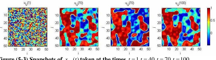
Consider the following diffusively coupled map model in a 2-dimensional L×L lattice (Kaneko, 1989)
))) 1 ( ( )) 1 ( ( )) 1 ( ( )) 1 ( ( ( * 4 )) 1 ( ( * ) 1 ( )
( , 1, 1, , 1 , 1
, t = − f x t− + f x− t− + f x+ t− + f x − t− + f x + t−
xij ij i j i j ij ij
θ θ
(5-9) where xi,j(t),i, j=1,...,L is the state at the discrete time t and the location of the
lattice(i, j). Here L is chosen to be 50 and θ is the parameter defining the coupling length. The dynamics of the CML at the lattice sites are governed by θ and the local map f . In this example, the mapping function f is chosen as the logistic map
2
1 )
(x ax
[image:11.595.89.507.127.301.2] [image:11.595.90.510.350.519.2]This model has been extensively studied and it is known that a rich set of bifurcations will occur as the bifurcation parameter a is changed when θ >0.3 (Kaneko, 1989, Guo and Billings, 2004). In this example, the parameters in (5-9) were set as a=1.5 andθ =0.4.
The CML model (5-9) was simulated with the parameters set above for 100 steps over the 50×50lattice I2starting from a randomly generated initial population and periodic boundary conditions. Snapshots of the spatiotemporal patterns at different times are shown in Figure (5-3). Here, the measurement function at the location of the lattice(i, j) is given as
) ( ) ( )
( , ,
, t x t t
yij = i j +εi j (5-11)
where the residualεi,j(t)denotes the measurement noise at the specific location(i, j)and time t.
Figure (5-3) Snapshots of xi,j(t)taken at the times t=1,t=40,t=70,t=100
The new model validation methods were implemented with N is set to be 2500. The outputs in (5-9) from four neighbouring sites were treated as inputs, and the input in
) ( 2 τ
φβu was selected to be a combination of four normalized inputs (similar to (5-7)).
) ( )
(
) ( )
(
) ( )
(
) ( )
(
1 , 4
,
1 , 3
,
, 1 2
,
, 1 1
,
t y t u
t y t u
t y t u
t y t u
j i j
i
j i j
i
j i j
i
j i j
i
+ − + −
= = = =
(5-12)
Figure (5-3) shows the results of the correlation tests for the CML model (5-9) )
( 2 τ
φβε and φβu2(τ) for the case where εi,j(t) was a totally random spatiotemporal
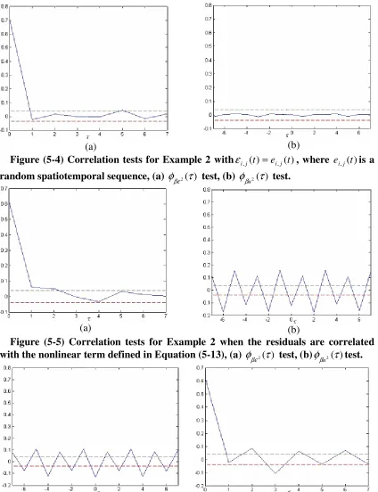
sequence. Figures (5-4), (5-5) show the correlation tests φβε2(τ)andφβu2(τ) under the two conditions where the residual εi,j(t) is random and correlated with the nonlinear terms defined in Equation (5-13) and Equation (5-14).
) 2 ( ) 1 ( 03 . 0 ) ( )
( , 1, 1,
,j t =eij t + yi− j t− yi− j t− i
ε (5-13) )
1 ( ) 1 ( 02 . 0 ) ( )
( , , ,
,j t =ei j t + yij t− yi j t− i
[image:12.595.93.509.286.402.2](a) (b)
Figure (5-4) Correlation tests for Example 2 withεi,j(t)=ei,j(t), where ei,j(t)is a
random spatiotemporal sequence, (a) φβε2(τ) test, (b) φβu2(τ) test.
(a) (b)
Figure (5-5) Correlation tests for Example 2 when the residuals are correlated with the nonlinear term defined in Equation (5-13), (a) φβε2(τ) test, (b)φβu2(τ)test.
(a) (b)
Figure (5-6) Correlation tests for Example 2 when the residuals are correlated with the nonlinear term defined in Equation (5-14), (a) φβε2(τ) test, (b) φβu2(τ) test.
[image:13.595.88.512.103.655.2]In this example, the new correlation tests are used to validate an identified CML model of a nonlinear spatiotemporal system described by a partial differential equation.
Consider the Lotka-Volterra predator-prey model in two dimensions (Wilson etc, 1993) described by the following parabolic PDE as
uv r v a v c v c v uv r u a u c u c u 2 2 22 21 1 1 12 11 + − ⋅ ∇ + ⋅ ∇ = − + ⋅ ∇ + ⋅ ∇ = • • (5-15)
where u=u(t,x,y)andv=v(t,x,y)present the prey population density and the predator population density at time t and location (x,y) respectively. The corresponding coefficients in the above PDE were set asa1 =0.47,r1 =0.024,a2 =0.76and r2 =0.023. The diffusive coefficients were set as c11 =c12 =0.1 andc21 =c22 =0.01 which signify
that the prey diffuses faster than the predators through the space domain.
The Lotka-Volterra equation (5-15) was numerically simulated on the space domain ) 1 , 0 ( ) 1 , 0
( × with the Neumann boundary conditions and initial conditions set as
≥ − + − = ≤ − + − = otherwise y x y x v otherwise y x y x u , 0 16 / 1 ) 2 / 1 ( ) 2 / 1 ( , 1 ) , , 0 ( , 0 16 / 1 ) 2 / 1 ( ) 2 / 1 ( , 1 ) , , 0 ( 2 2 2 2 (5-16)
The discrete observation for the identification are given by
15 ,... 2 , 1 ; 50 ,..., 2 , 1 , ), ( ) , , ( ) ( ) ( ) , , ( ) ( , , , , = = + ∆ ∆ ∆ = + ∆ ∆ ∆ = k j i k y j x i t k v k v k y j x i t k u k u j i j i j i j i β α (5-17) The numerical solution for (5-15) was sampled on the spatial grid ∆x=0.02,∆y=0.02
with a time step∆t =0.06.
In (5-17), αi,j(k) and βi,j(k) are random sequences with standard deviations
01 . 0 , 0058 . 0 = = β α σ
σ respectively. A CML model was identified by using an Orthogonal Forward Regression algorithm (Billings etc 1988, Guo and Billings 2004), and the results are shown in Table (5-1). In this example, for simplicity of illustration, only the model of subsystem u is investigated.
Table (5-1) Terms and parameters of the identified CML model for Example 3 and Subsystem u
Model Terms Estimated Parameters )
1 (
, k−
ui j 0.3161
Constant 0.0316
) 1 ( , − ∗ k
ui j ¶ 0.1681
2 )^ 1 (
, k−
ui j -0.3485
[image:14.595.95.502.587.708.2]The identified CML model in Table (5-1) can be expressed as.
( ) 0.3161 ( 1) 0.0316 0.1681 ( 1) 0.3485 ( 1) , ( )
2 , ,
,
, k u k u k u k e k
ui j = ij − + + ij − − ij − + ij
∗
(5-18) where ei,j(k) is the residual sequence. Figure (5-7), (5-8) (5-9) show some snapshots of the measured output, model predicted output (4-3) and the residuals at different times. As noted in Section 4, it can be seen from Figure (5-7) that the variance of ui,j(k)changes with the time k.
Figure (5-7) Snapshots of the measured output of the identified CML model Equation (5-18) taken at different times
Figure (5-8) Snapshots of the model predicted output of the identified CML model Equation (5-18) taken at different times
Figure (5-9) Snapshots of the residuals of the identified CML model Equation (5-18) taken at different times
[image:15.595.86.513.229.579.2]coefficient of ui2,j(k−1)was therefore changed from the correct value of −0.3485in Equation (5-18) to the incorrect or biased value of −0.3000in Equation (5-19).
) ( ) 1 ( 3000 . 0 ) 1 ( 1681 . 0 0316 . 0 ) 1 ( 3161 . 0 )
( ,
2 , ,
,
, k u k u k u k e k
ui j = ij − + + ij − − i j − + i′j
∗
(5-19) The correlation tests for (5-19) are given in Figure (5-11) and the incorrect estimate can clearly be detected in the model from the correlation functions φβε2(τ)andφβu2(τ) which are now located outside the 95% confidence limit.
(a) (b)
Figure (5-10) Correlation tests for identified model (5-18) in Example 3, (a) φβε2(τ)
test, (b) φβu2(τ) test.
(a) (b)
Figure (5-11) Correlation tests for identified model (5-19) in Example 3 with a biased estimate, (a) φβε2(τ) test, (b) φβu2(τ) test.
6
Conclusions
[image:16.595.88.510.228.611.2] [image:16.595.90.507.233.401.2]computing all the states over the whole lattice has been avoided by randomly selecting the data from both the time and space domain. Replacing the compound variable
) ( ) (t t
yi εi by the combination of two normalized variables ˆ 0()
t
yεi and εεi0(t) was shown to make the new correlation tests more practically feasible and robust for the spatiotemporal systems case where variances of the output and residual can be quite different. The new model validation methods have been developed for SISO and SIMO spatiotemporal systems, but the application to MIMO spatiotemporal systems is straightforward by introducing the ideas from MIMO temporal systems (Billings and Zhu, 1995).
Reference:
1. Aguirre, L.A., Billings S.A. (1994). Validating identified nonlinear models with chaotic dynamics, Int. J. Bifurcation and Chaos, 4, 109-125.
2. Aguirre, L.A., Billings S.A. (1995a). Retrieving Dynamical invariants from chaotic data using NARMAX models , Int. J. Bifurcation and Chaos, 5, 449-474.
3. Aguirre, L.A., Billings S.A. (1995b). Dynamical effects of over parameterization in nonlinear models, Physica D, 80, 26-40.
4. Billings, S.A. and Chen, S. and Kronenberg, M.J. (1988). Identification of MIMO non-linear systems using a forward regression orthogonal estimator. Int. J. Control,
49, 2157-2189.
5. Billings, S.A. and Coca, D. (2002). Identification of coupled map lattice models of deterministic distributed parameter systems. Int. J. Systems Science, 33, 623-634. 6. Billings,S.A. and Zhu,Q.M. (1994). Nonlinear model validation using correlation
tests. Int. J. Control, 60, 1107- 1120.
7. Billings,S.A. and Zhu,Q.M. (1995) Model validation tests for multivariable nonlinear models including neural networks. Int. J. Control, 62, 749-766.
8. Bohlin,T. (1971) On the problem of ambiguities in maximum likelihood identification.
Automatica, 7, 199-210;
9. Bohlin,T. (1978), Maximum power validation of models without higher order fitting.
Automatica, 14, 137-146.
10.Coca, D. and Billings, S.A. (2003). Analysis and reconstruction of stochastic coupled map lattice models. Phys. Lett. A, 31, 61-75.
11.Guo, L.Z. and Billings, S.A. (2004). Identification of coupled map lattice models of stochastic spatio-temporal dynamics using wavelets. Dynamical System, 19, 265-278. 12.Kaneko, K. (1985). Spatiotemporal intermittency in coupled map lattices. Prog.
Theor. Phys., 74, 1033-1044.
13.Kaneko, K. (1986). Turbulence in coupled map lattices. Physica D, 18, 475-476. 14.Kaneko, K. (1989). Spatiotemporal chaos in one-and two-dimensional coupled map
lattices. Physica D, 37, 60-82.
15.Mao, K.Z. and Billings, S.A. (2000). Multi-directional model validity tests for non-linear system identification. Int. J. Control, 73, 132-143.
16.Ostavik, S. and Stark, J. (1998). Reconstruction and cross-prediction in coupled map lattices using spatio-temporal embedding techniques. Phys. Lett. A, 247, 145-160. 17.Soderstrom, T. and Stoica, P. (1990). On covariance function tests used in system