Topics in General Relativity: Binary Black Holes and Hyperbolic Formulations of Einstein's Equations

Topics in general relativity: binary black holes and

hyperbolic formulations of Einstein's equations

Thesis by

Kashif Alvi

In Partial Fulfillment of the Requirements for the Degree of

Doctor of Philosophy

California Institute of Technology Pasadena, California

2002

Acknow ledgements

First and foremost, I would like to thank my parents Farhat and Mohammed Siddiq Alvi for their support and encouragement over the years, and especially for teaching me what is truly important in life. They have imprinted me with their high standards for personal conduct and achievement. They have always encouraged me to pursue my interests and dreams.

I am grateful to my advisor Kip Thorne for his guidance and support, and for providing a fruitful research environment. I am indebted to Lee Lindblom for suggesting the direction for the final research project in this thesis, and for guidance during its completion. I have collaborated with and benefited from discussions with Scott Hughes, Yuk Tung Liu, Arkadas Ozakin, Jongwon Park, and Mark ScheeL

Abstract

This thesis consists of three projects in general relativity on topics related to binary black holes and the gravitational waves they emit. The first project involves calculating a four-metric that is an approximate solution to Einstein's equations representing two widely separated nonrotating black holes in a circular orbit. This metric is constructed by matching a post-Newtonian metric to two tidally distorted Schwarzschild metrics using the framework of matched asymptotic expansions. The four-metric presented here provides physically realistic initial data that are tied to the binary's inspiral phase and can be evolved numerically to determine the gravitational wave output during the late stages of inspiral as well as the merger.

The second project is on the tidal interaction of binary black holes during the inspiral phase. The holes' tidal distortion results in the flow of energy and angular momentum into or out of the holes in a process analogous to Newtonian tidal friction in a planet-moon system. The changes in the black holes' masses, spins, and horizon areas during inspiral are calculated for a circular binary with holes of possibly comparable masses. The absorption or emission of energy and angular momentum by the holes is shown to have a negligible influence on the binary'S orbital evolution when the holes have comparable masses. The tidal-interaction analysis presented in this thesis is applicable to a black hole in a binary with any companion body (e.g., a neutron star) that is well separated from the hole.

Contents

Acknowledgements

Abstract

1 Introduction 1.1 Bibliography

2 An approximate binary black hole metric 2.1 Introduction . . . . 2.2 Near zone and racliation zone metrics . 2.2.1 Binary system parameters .. .

2.2.2 Demarcation of four regions in spacetime 2.2.3 Near zone metric in harmonic coordinates 2.2.4 Near zone metric in corotating coordinates 2.2.5 Radiation zone metric in harmonic coordinates 2.2.6 Radiation zone metric in corotating coordinates. 2.3 Tidal deformation of the first black hole . . . .

2.3.1 Tidal fields of the companion black hole 2.3.2 Schwarzschild perturbation . . . . 2.4 Distorted black hole metrics in corotating coordinates

2.4.1 2.4.2 2.4.3

Buffer zone coordinate transformation . . Internal metric in corotating coordinates . Metric near the second black hole. 2.5 Results and discussion

2.6 Bibliography . . .

3 Ingoing coordinates for binary black holes 3.1 Introduction . . .

3.2 Ingoing coordinates .

3.3 'Transformation to corotating coordinates 3.4 Bibliography . . .

4 Energy and angular momentUlll flow into a black hole in a binary

4.1

Introduction .

4.2 Framework .

4.3 Stationary companion

4.4

Equatorial orbits .. .

4.4.1

Instantaneous rates.

4.4.2

Total changes during inspiral

4.4.3

Effect on orbital evolution .

4.5

Non-equatorial orbits . . . .

4.5.1

Description of orbit 4.5.2 Approximation scheme. 4.5.3 Orbit-averaged quantities

4.6

Discussion..

4.7

Bibliography

5 First-order symmetrizable hyperbolic formulations of Einstein's equations includ-ing lapse and shift as dynamical fields

5.1

Introduction .

5

.2

System I . ..

5.2

.1

Fischer-Marsden system

5.2.2

Generalized harmonic coordinates

5.2

.3

System I ..

5.2.4

Initial data

5.2.5

Hyper bolicity of system I

5.3

System II

....

5.4

Future directions

5.5

Bibliography

..

List of Figures

List of Tables

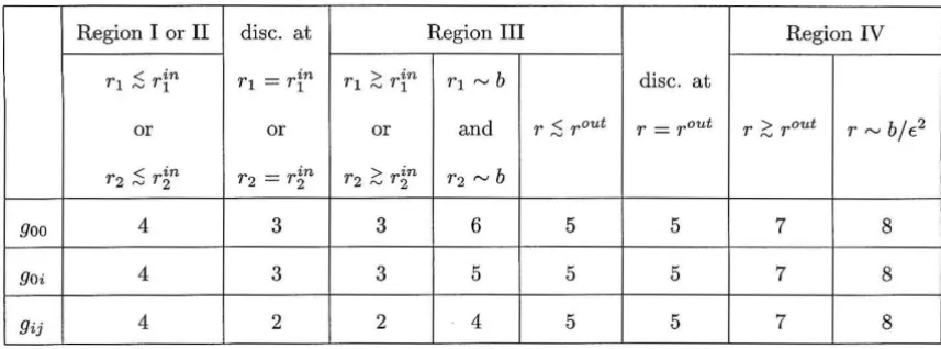
2.1 Errors and discontinuities in the metric components in corotating coordinates. Num-bers denote orders in ~ = (m/b)1/2; e.g., 4 denotes O(~4). The last two columns contain normalized errors. . . . . . . . . . . . . . . . . . .. 34

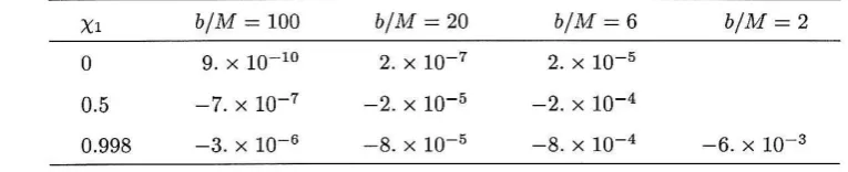
4.1 Normalized change 6.81/ M'f in spin evaluated at b/ M =100,20, and 6 for an equal-mass binary with iN .

8

1 = 1. For rapidly rotating holes (Xl = X2 = 0.998), this change is also evaluated at b/M = 2. . . . . . . . . . . . . . . . . . . 52 4.2 Normalized change 6.M1/Ml in mass evaluated at b/M=100, 20, and 6 for an

equal-mass binary with i N . 81 = 1. For rapidly rotating holes (Xl = X2 = 0.998), this change is also evaluated at b/M = 2. . . . . . . . . . . . . . 52 4.3 Normalized change 6.A1/Al in horizon area evaluated at b/M=100, 20, and 6 for an

equal-mass binary with iN

.8

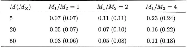
1 = 1. For rapidly rotating holes (Xl = X2 = 0.998), this change is also evaluated at b/M = 2 . . . .

4.4 Change 6.N in the number of gravitational-wave cycles due to black hole absorp -tion/emission, for various values of total mass M and mass ratio Ml/M2. The initial separation is such that the wave frequency is 10 Hz and the spins satisfy Xl

=

X2

=

52

Chapter

1

Introd uction

The central theme in this thesis is binary black holes. The exact evolution of these binaries is still

an unsolved problem in general relativity. Solution of this two-body problem is important not only

as a matter of principle, but also as a practical concern. A full solution of the problem will not

only give insights into Einstein's theory of gravitation, but also provide gravitational waveforms

that will be used in several stages of data analysis for gravitational wave detectors such as the Laser

Interferometer Gravitational-Wave Observatory (LIGO) and the Laser Interferometer Space Antenna

(LISA). Since binary black holes are expected to be among the primary sources of gravitational waves

for these interferometric detectors, it is important to try to solve this problem using all available

techniques, including approximate analytical methods and numerical simulations.

One regime in which the evolution of binary black holes is well understood is the early inspiral

phase. In this phase, the holes' separation is still much larger than the binary's total mass, and

post-Newtonian expansions can be used to analyze the system. Eventually radiation reaction drives

the holes together and the post-Newtonian approximation fails. The binary's subsequent evolution

must be studied numerically. As the holes merge and begin to settle down into a stationary final

state, black hole perturbation theory becomes increasingly effective in describing the dynamics.

The approximate analytical techniques of post-Newtonian expansions and black hole perturbation

theory, which are applicable before and after the merger, will have to be combined with numerical

simulations of the merger to yield complete waveforms for binary black hole coalescences.

The research work done for this thesis is motivated by the need to calculate the gravitational

wave output from binary black holes. The main chapters of this thesis deal with various aspects

of these binaries. Chapter 2 is concerned with the interface between the post-Newtonian inspiral

and the fully nonlinear merger. It has been argued [1] that post-Newtonian expansions begin to

fail during the late stages of inspiral, before the black holes begin to merge. The gap between the

failure of post-Newtonian expansions and merger has been called the intermediate binary black hole

region. This gap consists of approximately 10-20 orbits and 100-250 radians of gravitational-wave

region lies in the frequency band of optimal LIGO sensitivity [1]. Since binaries with total mass in

the range 10-40 M0 are most likely to be the first detected by LIGO [1], it is important to come up with techniques to fill in the intermediate binary black hole gap.

Numerical solution of this problem will require initial data that accurately represent binary black

holes that have spiraled in from large separation. Furthermore, these initial data will have to be

linked to the early inspiral phase of the binary and to the binary'S initial parameters (e.g., masses

and spins) during this phase. Post-Newtonian expansions alone are not capable of providing such

initial data because they treat the two bodies as point particles. These expansions do not take into

account the spacetime structure near the black holes' horizons. Furthermore, the initial data being

used currently in numerical simulations (see [2] for a recent review; see also [3]) are not astrophysicaliy realistic: these data typically depend on unphysical assumptions on the metric such as conformal

flatness for the spatial metric. As a result, these data contain spurious gravitational wave energy

of the order of the total energy radiated to infinity during coalescence [3]. These data also contain spurious deformations of the black holes, which will lead to black hole pulsations. A different method

is therefore required to provide initial data at the interface between the post-Newtonian inspiral and the fully nonlinear merger.

In Chapter 2, I present such a method. I derive a 4-metric that is an approximate solution to Einstein's equations representing two widely separated nonrotating black holes in a circular orbit.

This metric is constructed by matching a post-Newtonian metric to two perturbed Schwarzschild

metrics using the framework of matched asymptotic expansions. The spacetime metric is presented

in a single corotating coordinate system that covers the radiation and near zones as well as the regions

near the black holes, up to their apparent horizons. In Chapter 3, I define an ingoing coordinate transformation that extends this corotating coordinate system through the holes' horizons and into

their interiors. The motivation for using ingoing coordinates is that numerical simulations of black holes require the computational grid to extend inside the horizons. Thus, the coordinate system

used near the black holes in Chapter 2 is not suitable for numerical relativity.

Initial data extracted from the binary black hole 4-metric presented in Chapters 2 and 3 have the

advantages of being linked to the early inspiral phase of the binary system, and of not containing

spurious gravitational waves or spurious deformation of the black holes. Besides providing initial

data, this 4-metric serves as a check on the early stages of numerical evolution of these data. Plans are underway to implement and evolve these initial data in collaboration with L. Kidder, H. Pfeiffer,

Hyperbolic systems will be discussed in further detail below.

It should be kept in mind that the 4-metric presented in Chapters 2 and 3 is an approximate solution to Einstein's equation, and the approximation gets worse as the ratio of the binary's total

mass to the holes' separation gets larger. A complete error analysis on the metric is given in Chapter 2. The accuracy of the metric can be improved by restricting to large separations relative to total mass (note that the code being developed by Kidder, Pfeiffer, and Scheel can handle these large

separations because pseudospectral collocation techniques require far fewer spatial grid points than straightforward finite difference techniques), or by taking the calculation in Chapters 2 and 3 to higher order.

Chapter 4 examines the tidal interaction of binary black holes during the inspiral phase. As the holes spiral in, they distort each other with their tidal fields. This distortion causes the holes' horizon areas to increase slowly during inspiral, and results in the flow of energy and angular momentum

into or out of the holes. This process is analogous to Newtonian tidal friction in a planet-moon system

[6-9].

The tidal-interaction analysis of Chapter 4 is applicable to a black hole in a binary with any companion body (e.g., a neutron star) that is well separated from the hole. The changes

in the black hole's mass, spin, and horizon area during inspiral are calculated for a hole in a circular binary with a companion body of possibly comparable mass.

The orbital evolution of binary black holes is affected by the absorption/emission of energy and angular momentum by the holes. In particular, the number of orbits- and hence the number of gravitational-wave cycles emitted to infinity- changes when black hole absorption/emission is accounted for. In Chapter 4, this effect is estimated for a circular, nearly Newtonian binary with spins aligned or anti-aligned with the orbital angular momentum. The binary is assumed to lose orbital energy and angular momentum to infinity via Newtonian quadrupole radiation, and to the

black holes via tidal interaction. The conclusion in Chapter 4 is that black hole absorption/emission

of energy and angular momentum during inspiral may not be an important effect for the detection (by LIGO) and analysis of gravitational waves from comparable-mass black holes. However, in the extreme-mass-ratio limit, black hole absorption/emission can strongly influence the binary's orbital evolution and thus is an important effect for LISA [10].

The results in Chapter 4 also provide some information on the interface between the inspiral and merger phases of binary evolution. As mentioned above, current numerical simulations of binary black holes use initial data that are not tied to the inspiral phase and to the post-Newtonian expansions used to describe it. Therefore, one needs to relate the masses, spins, and horizon areas of the black holes present in currently used initial data to the corresponding quantities when the holes

were infinitely separated. For this purpose, it is necessary to know how these quantities change

The final chapter of this thesis is concerned with first-order hyperbolic formulations of Einstein's

equations, which are promising as a basis for numerical simulation of binary black holes. The basic framework for the theory of first-order hyperbolic systems is as follows. Consider a system of

equations of the form

where u is a column vector composed of the unknown fields (which could include metric components

and extrinsic curvature components, for example), and the matrices Ai and column vector F can

depend on space and time and on the fields but not their derivatives. Pick a unit spatial covector ~i

and compute the eigenvalues>. of the matrix Ai~i; >. are the characteristic speeds in the direction

~i. If all the eigenvalues are real for each ~i' then the system is called weakly hypberbolic. If in

addition, Ai~i has a complete set of eigenvectors for each ~i, the system is called strongly hyperbolic.

If the matrices Ai are symmetric, the system is called symmetric hyperbolic. If there is a positive definite symmetric matrix H such that H A i are symmetric, the system is called symmetrizable

hyperbolic. The initial value problem is well posed for strongly, symmetric, and symmetrizable

hyperbolic systems-that is, for these systems the problem has a unique solution that depends

continuously on the initial data [11]. The initial value problem is not well posed for weakly hyperbolic systems [11].

First-order hyperbolic systems have been used in the past to prove that general relativity has a

well-posed initial value formulation [12, 13]. There has been considerable interest recently in these systems because of the advantages they offer to numerical simulations [14, 15]. The main advantage

is that imposing physical boundary conditions is much easier in the framework of a hyperbolic

system than a non-hyperbolic one. This is especially true for boundary conditions inside a black hole horizon [14, 15]. Indeed, if the hyperbolic system has only physical characteristic speeds -that is, if the characteristic fields propagate only on the light cones of spacetime or normal to the hypersurfaces of constant time- then the boundary condition inside the horizon on fields propagating

into the numerical grid has no effect on the dynamics outside the horizon. Therefore, in this case, any

convenient boundary condition can be imposed inside the horizon. This is a significant advantage when simulating black holes.

Numerical solution of Einstein's equations is typically done in the framework of a 3+ 1 split of

spacetime (see, e.g., [16, 17]). In this framework, spacetime is foliated by spacelike hypersurfaces that represent constant time slices. The spacetime metric is expressed as

(3j ) rij ,

and (3i

=

/ij(3j. The lapse and shift can be freely chosen when evolving initial data, and are there-fore called gauge fields. Freedom in choosing these gauge fields, i.e., gauge freedom, corresponds to freedom in choosing coordinates for spacetime. This freedom can be used in numerical evolutions for a variety of purposes, e.g., to prevent the occurrence of coordinate singularities [18], to reduce coordinate shear [18], and to adapt the coordinate system to the particular problem under consider-ation. When simulating black holes, it is helpful to choose the shift so that numerical grid points do not fall into the holes. When simulating binary black holes, it may be advantageous to implement gauge conditions which generate corotating coordinates [1, 19].

In previous work, the gauge fields have typically not been considered part of the hyperbolic system and have been prescribed independently. Some of the favored gauge prescriptions in numerical relativity [18, 19] require solution of elliptic equations for the lapse and shift, which is expensive computationally. It would be more efficient to evolve the gauge fields as part of the hyperbolic system. However, it is important to keep some freedom in choosing the gauge in order to allow the coordinates to be adapted to fit specific needs. In Chapter 5, I present two first-order symmetrizable hyperbolic systems for Einstein's equations which include the lapse and shift as dynamical fields and allow four functions of spacetime to be specified freely in the gauge prescription. The first hyperbolic system is a modification and generalization of the work of Fischer and Marsden [12]; this system uses generalized harmonic coordinates and evolves 50 fields. It is promising as a basis for numerical work. The second system is based on the work of Kidder, Scheel, and Teukolsky [5] and Lindblom and Scheel [20]; it evolves 70 fields. This system is not practical for numerical implementation. Its main use is theoretical: it allows one to show that any solution to Einstein's equations in any gauge can be obtained using hyperbolic evolution of the entire metric, induding the gauge fields. Both systems have only physical characteristic speeds.

An important future research direction is to study and understand the stability of numerical

implementations of the first hyperbolic system presented in Chapter 5. It has been shown in previous work [5] that some hyperbolic systems are more stable than others when used to simulate black holes in three spatial dimensions. The reasons for this behavior are not yet understood. Another future research direction is to explore how to use the freedom in gauge choice in the first hyperbolic system of Chapter 5 to control the coordinate system.

1.1

Bibliography

[1]

P. R. Brady, J. D. E. Creighton, and K. S. Thorne, Phys. Rev. D 58, 061501 (1998).

[3] H. P. Pfeiffer, G. B. Cook, and S. A. Teukolsky, gr-qc/0203085.

[4] H. P. Pfeiffer, L. E. Kidder, M. A. Scheel, and S. A. Teukolsky, gr-qc/0202096.

[5] L. E. Kidder, M. A. Scheel, and S. A. Teukolsky, Phys. Rev. D 64, 064017 (2001).

[6] S. W. Hawking and J. B. Hartle, Commun. Math. Phys. 27, 283 (1972).

[7]

J.

B. Hartle, Phys. Rev. D 8, 1010 (1973).

[8]

J

.

B. Hartle, Phys. Rev. D 9, 2749 (1974).

[9] Black Holes: The Membrane Paradigm, edited by K. S. Thorne, R. H. Price, and D. A.

Mac-donald (Yale University Press, New Haven, 1986).

[10] S. A. Hughes, Phys. Rev. D 64, 064004 (2001).

[11] B. Gustafsson, H.-O. Kreiss, and J. Oliger, Time Dependent Problems and Difference Methods

(Wiley, New York, 1995).

[12] A. E. Fischer and J. E. Marsden, Commun. Math. Phys. 28, 1 (1972).

[13] H. Friedrich, Commun. Math. Phys. 100, 525 (1985).

[14] H. Friedrich, Class. Quantum Grav. 13, 1451 (1996).

[15] A. Anderson and J. W. York, Phys. Rev. Lett. 82, 4384 (1999).

[16] C. W. Misner, K. S. Thorne, and J. A. Wheeler, Gravitation (Freeman, San Francisco, 1973).

[17] J. W. York, in Sources of Gravitational Radiation, edited by L. L. Smarr (Cambridge University Press, Cambridge, 1979), p. 83.

[18] L. Smarr and J. W. York, Phys. Rev. D 17, 2529 (1978).

[19] D. Garfinkle, C. Gundlach, J. Isenberg, and N. OMurchadha, Class. Quantum Grav. 17, 3899

(2000).

Chapter 2

An approximate binary black hole metric

Published as K. Alvi, Phys. Rev. D 61, 124013 (2000).

Abstract

An approximate solution to Einstein's equations representing two widely separated nonrotating

black holes in a circular orbit is constructed by matching a post-Newtonian metric to two perturbed Schwarzschild metrics. The spacetime metric is presented in a single coordinate system valid up to the apparent horizons of the black holes. This metric could be useful in numerical simulations of

binary black holes. Initial data extracted from this metric have the advantages of being linked to

the early inspiral phase of the binary system, and of not containing spurious gravitational waves.

2.1

Introduction

One of the outstanding issues in gravitational wave research is calculating the wave output from

the last stages of inspiral of binary black holes. This intermediate binary black hole problem has

been discussed by Brady, Creighton, and Thorne [1]. The purpose of this paper is to provide an approximate four-dimensional binary black hole metric from which initial data can be extracted and

evolved numerically into and through the intermediate binary black hole region.

The approach I take is based on the work of Manasse [2] and D'Eath [3, 4]. I consider two widely separated nonrotating black holes in a circular orbit. The black holes' mass ratio is not restricted-they can have comparable masses. However, the masses are assumed to be milch smaller than the distance between theml

. As a result spacetime can be divided into four regions, each with its own approximation scheme to solve Einstein's equations. There is a strong-gravity region near each of the black holes which is described by the Schwarzschild solution plus a perturbation due to the companion's tidal field. This perturbation is constrained to satisfy the linearized Einstein equations

about the Schwarzschild metric. The companion black hole's electric-type and magnetic-type tidal fields are both taken into account in calculating the perturbation.

Outside the strong-gravity regions but within the near zone, the metric can be approximated by a post-Newtonian expansion. Further out is the radiation zone which contains outgoing gravitational waves and can be described by a post-Minkowski expansion of the metric.

There are overlap zones in this spacetime where the regions described above intersect in pairs. In the overlap zones, two different approximation schemes-one from each of the two intersecting regions- are both valid. The perturbative expansions produced by the two approximation schemes are matched in the overlap zones using the framework of matched asymptotic expansions. The post-Newtonian near-zone metric-taken from [5]-and the radiation-zone metric-taken from [6]-already match in their overlap region. In this paper, the post-Newtonian near-zone metric is matched to a perturbed Schwarzschild metric in the matching or buffer zone surrounding each black hole. This yields information on the asymptotic behavior of tbe Schwarzschild perturbation at large distances from the horizon, and on the coordinate transformation between the two buffer-zone coordinate systems.

The Schwarzschild perturbation and coordinate transformation are not uniquely determined. However, a different choice of transformation, and hence a different form of Schwarzschild pertur-bation, should still represent the same physical situation. In other words, different perturbations that match to the post-Newtonian near-zone metric are expected to be related via gauge transforma-tions. For the purposes of this paper, it is sufficient to find one transformation and one Schwarzschild perturbation associated with each black hole that result in a match between the post-Newtonian near-zone metric and the distorted-black-hole metrics.

An approximate spacetime metric is put together by joining the regional metrics at some specific 3-surfaces in the matching zones. The final 4-metric is written in a single coordinate system valid up to (but not inside) the apparent horizons of the black holes. This metric is useful not only as a source of initial data for numerical evolution, but also as a check on the early stages of such an evolution.

It has been suggested that numerical simulation of binary black holes should be performed in corotating coordinates [1]. For this reason the metric in final form is given in corotating coordinates. The binary black hole spacetime can be sliced and spatial coordinates chosen in any convenient way when extracting initial data from the metric. (Asymptotically inertial coordinates can be used, for example.)

the metric presented here.

Initial data from this metric have the additional advantages of not containing spurious

gravita-tional waves and of reliably describing the physical situation of coalescing binary black holes. The

accuracy of this description can be improved by taking the calculation in this paper to higher orders.

In Sec. 2.2, the near-zone and radiation-zone metrics are written down. In Sec. 2.3, the first

black hole's tidal deformation is calculated. In Sec. 2.4, the buffer-zone coordinate transforma

-tions are determined, and the distorted-black-hole metrics are written in corotating post-Newtonian

coordinates. The full spacetime metric is summarized in Sec. 2.5.

2.2

Near zone and radiation zone metrics

Blanchet and collaborators ( [7] and references therein) and Will and Wiseman [6] have calculated

in detail the near-zone and radiation-zone gravitational fields of compact binary systems. The

approach taken by Will and Wiseman is particularly useful here because they use a single coordinate

system- harmonic coordinates-to cover both the near zone and the radiation zone. As a result,

expressions for the radiation-zone metric components taken from [6] automatically match (to some

finite order) the harmonic-coordinate, post-Newtonian, near-zone metric components calculated in

[5]. For this reason I work initially in harmonic coordinates (t', x', y', z') with the origin of the

spatial coordinates placed at the binary system's center of mass. I use only the first post-Newtonian

(lPN) metric, not the full 2.5PN metric given in [5]2. Consistently with this, I put the black holes

on Newtonian trajectories: they are taken to be in circular orbits with Keplerian orbital angular

velocities. Moreover, I use the post-Newtonian metric for point-like particles; in the near zone, I

ignore the black holes' internal structure. The near-zone gravitational effects of the black holes'

multipole moments can in principle be computed by matching out to the near zone the

tidally-distorted Schwarzschild metrics obtained in this paper. However, these effects are too small to be

included in this paper; this is discussed further in Sec. 2.4.2.

2.2.1

Binary system parameters

Label the black holes BH1 and BH2, and let ml and m2 be their respective masses. Define

(2.1)

Denote the harmonic-coordinate trajectories of the black holes by x~ (t') for A

=

1,2 and j

=

1,2,3.

In other words, x~ (t') are the spatial coordinates at time t' of the center of attraction of the

gravitational field of black hole A.

In this section, boldface letters are used to denote spatial coordinates. For example XA = (x~,x~,x~)

=

(XA,YA,ZA). The notation

a·

b is used for the quantity 6_{jk a}j_{bk , and}

lal

_{is by}

definition (a· a)1/2.

Denote the black holes' separation IXl -

x21

by b. The circular, Newtonian trajectories of the

black holes are

where

and

Xl(t') = m2b(t'),

m

b(t')

=

Xl(t') - X2(t')

=

b(coswt', sinwt', 0)

w

=fi

is the Keplerian orbital angular velocity. Define

€

{i,

T = (X'2

+

y,2

+

z'2)1/2,

TA

lx' - x

AI, nA = x' -XA TA dXA

VA = IVAI,

VA =

dt' ,

V Vi - V2 = €( - sinwt', coswt', 0),

for A = 1,2. By assumption, €

«

1.

2.2.2

Demarcation of four

regions

in

spacet

ime

(2.2)

(2.3)

(2.4)

(2.5)

Let us first fix precisely four regions in this binary black hole spacetime; each of these regions will

receive a metric calculated as an approximate solution to the Einstein equations. With such a

partition of spacetime in mind, define the inner limits rin

=

vmlb and T~n

=

Vm2b. These are just

convenient choices for the inner limits. The important property rin has is that both Tin

/b

-t 0 and mdrin -t 0 as mdb -t O. Similarly r~n /b -t 0 and m2/r~n -t 0 as m2/b -t O. Also define the

outer limit rout = _Ac/27r = b/2E, where Ac = 7r

/w

is the characteristic wavelength of gravitational

radiation emitted by the binary system.

Divide spacetime into four regions that are bounded by the black holes' apparent horizons and

the surfaces Tl = Tin, r2 = r~n, and T = rouL (i) the region rl

<

rin (but outside the apparent horizon ofBH1), labeled region I; (ii) the region r2

<

r~n (but outside the apparent horizon ofBH2),

labeled region II; (iii) the subset of the near zone specified by rl

>

Tin, 7'2

> T;n,

and r

<

Tout,

r=rout

Region IV Region III

-,

r

1

=r/"

, ,

,

\

/

,

I

,

/ _Region

n

,

/

/ ,

,

Region I

,

,

,

\

•

BH2

_,

•

BHl

_,

,

/

,

, /

/

,

/ / r₂ = r{" \

_,

,

Zone , Zone

---

----

--b

Figure 2.1: Schematic illustration of the various regions in the binary black hole spacetime. Regions I, II, III, and IV are demarcated by solid lines; the buffer zones are bounded by dashed lines.

III and overlaps with regions I and II; the radiation zone corresponds to region IV. The buffer zone around black hole A contains r A

=

r t and satisfies mA

«

r A

«

b. These regions of spacetime are illustrated in Fig. 2. L

2.2.3

Near zone metric

in

harmonic coordinates

In the near zone, the 1PN harmonic-coordinate metric with two pOint-like particles representing the black holes is [5]

90'0'

gO'i'

gi'j'

This metric presumably differs in the near zone by a small amount from an exact solution to the Einstein equations representing binary black holes. I take the neglected terms in the 2.5PN metric [5] to be an estimate of the errors in the 1PN metric (2.6).

magnitude of these terms at various places in region III. If r A ~ r:r ~ bE (here and henceforth "~,,

means "is of the order of" and a ~ b means a

>

b and a ~ b) for A

=

1 or 2, then the error in 90'0'

(denoted 890' 0') is of 0 ( E3) and comes from neglecting a term of the form m ~ / r~. If both r1 ~ b

and r2 ~ b, then 890'0' ~ E6 Finally, if r;S rout ~ b/€ (so that r A ~ b/€ for A = 1 and 2), then the error 690'0' ~ €5 arises from neglecting the radiation reaction potential. Note that it is reasonable

to consider the "absolute" errors 891""' in the metric components since the coordinate system being

used is asymptotically inertial and the errors are only calculated in regions of weak gravity where

deviations from a flat metric are small.

A similar analysis for 90'i' yields 890'i' ~ €3 if r A ~ r:r for A = 1 or 2, 890'i' ~ €5 if both r1 ~ b and r2 ~ b, and 890'i' ~ €5 if r ;S rout. Lastly, 89i' j' ~ €2 if r A ~ r:r for A = 1 or 2 (this comes from

neglecting a term of the form m~/r~ in 9i'j'), 69i'j' ~ €4 if both 1'1 ~ b and r2 ~ b, and 69i'j' ~ €5

if r ;S rout.

2.2.4

Near zone

metric

in

corotating coordinates

The metric (2.6) is transformed to corotating coordinates (t, x, y, z) defined by

t' t, x'

=

x coswt - y sinwt,

y' x sinwt

+

y coswt, Zl

=

z. _(2.7)

In terms of the new coordinates,

(2.8)

Putting the expressions (2.2)-(2.5) in Eq. (2.6) and transforming to corotating coordinates gives

where, in terms of the new coordinates, the quantities r A are

(2.10)

throughout the near zone, which includes the buffer zones around the black holes.) It remains to

specify the metric in regions I, II, and IV. I postpone until Sec. 2.2.6 discussion of the errors Jgi"V

in the metric components in the new, rotating coordinate system (t, x, y, z).

2.2.5

Radiation zone metric in harmonic coordinates

The radiation-zone metric can be extracted from [6]. In that paper, a potential hi"' v' is defined by

(2.11)

where 'rJi"'V' =diag(-l,l,l,l), gi"'V' is the spacetime metric, and g' = det(gi"'v')' Equation (5.5) of [6] gives hi"' v' in the radiation zone in harmonic coordinates (t', x', y', Zl) for a system of several bodies. After correcting a typo in that equation,3 I specialize to a system of two bodies of masses ml and

m2 in a circular orbit specified by Eqs. (2.2)-(2.5). This yields4

hO'O'

(t',

x', y', z')

hO/if (tl, Xl, y', z')

hi'i' (t',x',y',z')

==

where

m

=

m(l - p./2b), u' = t' - r, n '

=

x'/r (2.13)

and

2

Qijk

=

L

mAx~x~x~

=

- p.(Jm/m)bibibk, A=l

2 2

Ji

==

L

mAEilmX~VA = f-Lf.ilmblvm,

A=l

Jij =

L

mAEilmx~VAX~ = _p.(Jm/m)Eilmb1vmbi. A=l

(2.14)

Putting the expressions (2.14) in Eq. (2.12) and using Eqs. (2.2)-(2.5) gives

4m

+ 7m

2

+

2p. {2(nl . V)2 _ 2m (n' . b)2

+

~(n'

_{. b)(n' . v)}

+

12 [3(n' . b)2 - b2] }

r r2 r b3 _{r r}

+

2p. Jm {7m (n' . b)2(n' . _{v) _ 2(n' . v)3}

+

~(n'

. b)

[6~

(n' . b)2 - 12(n' . v)2 - m_b]

r m ~ r b

+

~(n"

v)

[b

2 _{- 5(n'· b)2]}

₊

_{13 (n' · b)}

_[3b

2

- 5(n'· b)2]},

r2 r

3The term 4m/r' in the expression for hOD should instead be 4mjr'.

14

hO'i' =

4:

{[(n' .v) +

~(n'

.b)] Vi -

~(

n'

.b)bi }

2J.1.

am

{

m ( ' ) [ ( ' ) i ( ' ) i] , 2 i

-

rm

-

b3 n . b 3 n . b v + 4 n . vb + 2(n . v) v

1 [ ( ' )(' ) i 3m ( ' )2 i m i] 1 [ ( ' )2

2]

i}

+:;: 6 n . b n . v V -

b3

n . b b + Z;b + r2 3 n . b - b v ,

hi'jl m

2

,i'J 4J.1. [ i J m bid] 2J.1.

am

{

6m ( , b) (id)

- n n

+

-

v v - - fF

+ -

-

-

n · v fF

r2 r b3 r m b3

+ [

(n'. v)

+

~(n'.

b)]

(~b

ib1-

2viv J) }, (2.15)

where v and b are evaluated at the retarded time u' = t' - r.

The metric g/.l-'v' can be gotten from Eq. (2.15) as follows: from Eq. (2.11) we have

(2.16)

Take the determinant of both sides of Eq. (2.16); this yields g' = det(rlV

' - h/.l-'V'). So g' can be

calculated once h/.l-'v' is known, and then g/.l-'V' can be gotten from Eq. (2.16). Inverting the matrix

g/.l-'V' gives the spacetime metric gl"V'.

When performing these calculations, I keep all terms of the form m3-p/2b-3(1-p/2)r-p for integer

p

>

O. I also keep- at each order in r- all terms that are of lower order in m/b than this, and throw away terms of higher order in m/b. This means in particular that no terms of O(r-5) are kept. This

scheme of organizing terms is consistent with the ordering of terms in Eq. (5.5) of [6].

The result of these calculations is the following radiation-zone metric in harmonic coordinates:

90'0' -1 + -2m - 2m- - + - 2 n . v - - n . b + - n . b n . v

2

J.I. { ( ' )2 2m(, )2 6(, )(' )

r r2 r b3 r

+

~

[3(n'. b)2 _ b2_{] } +}

!!:.om{(

n'

_{.v) [7m(n'. b)2 _ 2(n'. v)2 _ m]}

r2 r m b3 b

+ - n · b - n · b -6n·v 2 ( ' )

[3m

('

)2 ( ' )2 - -

m

]

r b3 _b

+

:2

(n' · v)

[b

2 - 5(n'· b)2] +

:3

(n'· b)

[3b

2 - 5(n'· b)2]},

gO'i' - -; {[(n'. v) +

~(n'

.

b)] Vi -

~(n'.

b)bi}

2J.1.

am

({

('

2 3m ( ' )2 6 ( , b) ( ' ) 1 [3( 'b)2

b2]}

i + - - 2 n . v) - - n . b + - n· n· v + - n· - V

r m b3 r r2

+ { -

~r:

(n' . b)(n' . v) +

~

[1 - :2 (n' . b)2])

b}

+

~O::

{(n' .v)

[7b~(n"

b)2 - 2(n' 'V)2

+

7]

+

~(n'

·b)

[~(n"

b)2 - 2(n'.v)2]

+

:2 (n' . V) [b2 - 5(n' . b)2]

+

r13 (n' . b) [3b2 - 5(n' . b)2] } )

+

Oi'

(1

+

2m

+

m2)

+

m

2

n'in'j+ 4J.L (Vivj _ mbibi)

J r r2 r2 r b3

+ 2J.L Om {6m (n' . b)v(ibi)

+

[(n' . v)

+

~(n'

. b)] (m bibi _ 2vivj)}

r m b3 _{r b}3 _' (2.17)

where v and b are evaluated at the retarded time u' = t' - r.

The errors Og",v' in these metric components in region IV can be estimated by computing the

orders of magnitude of neglected terms, which are of the form m3-v/2b-3(1-v/2)r-p(m/b)n/2 for

integers p

>

0 and n

>

O. These terms include m 3/b2r, £m2 /r2, m 2b/r3, etc. This gives Og",v' ~ £7

for r;::; rout ~ b/£, Og",v' ~ £8 for r ~ b/£2» rout, and og",v' «£8 for r » b/c2

2.2.6

Radiation zone metric in

corotating

coordinates

Substituting the expressions (2.2)-(2.5) into the metric (2.17) and transforming this metric to coro-tating coordinates (t, x, y, z) [defined in Eq. (2.7)] gives

where

dt2 - 1 + - 1 - - - - +A+- £B-2cMD [

2m ( J.L) 2m2 2c2

r 2b r2 b

+W2(X2 _+y2)E

₊

_{_£2N +£2M 2S} E4 _{_ _} 1211Er-_ _ £2M

5 _{c5m ]}

b2 r 2b2 m

+ 2dt (E[Sin(Wr)dx

+

cos(wr)dy]B

+

b[cos(wr)dx - sin(wr)dy]D

+

w(xdy - ydx)E

3

+ £b £[sin(wr)dx

+

cos(wr)dy]N - EbM[cos(wr)dx - sin(wr)dy]S

+ 6J.L 2E

4

Om £ [(x cos 2wr - y sin2wr)dx - (x sin 2wr

+

y cos _2wr)dY])

r b m

m2

+ E(dx2

+

dy2

+

dz 2)

+

""4 (xdx

+

ydy

+

Zdz)2

+

E2[sin(wr)dx

+

cos(wr)dyj2 N

r

+ b2[cos(wr)dx - sin(wr)dy]2S

+

12~E3

Om £[cos(wr)dx _ sin(wr)dy](sin(wr)dx

+

cos(wr)dy], (2.18)

r m

A = .!:!:.. {2£2 [M2 _ £2]

+

6b£ M£

+

b 2

[3£2 _ r2] }

+

.!:!:.. c5m { b 3

£ [3r2 _ 5£2]

r3 r r2 r4 m r3

+ 3b2E M [r2 _ 5£2]

+

2m £ [3£2 _ 6M 2 _ r2]

+

E3 M [7£2 _ 2M2 - r2]},

r2 r

B _

4~

[EM

+

~£]

+

2~

Om {c2 [2M2 _ 3£2]

+

6bE M£

+

b: [3£2 _ r2]},

D

₌

2/-L€2

e£ -

.!.

8m {4€ £M +

.!.

[3£2 _ r2] } )

r2 b r m b r '

E

1+-2m ( 1 - -/-L) + -m + A + - - -£+€M

2

2/-L€2 8m [b ]

r 2b r2 r2 m r · '

N

₌

4/-L { - 1 - 8m - [€ -M +

-

b ] }

£

,

r m r r2

S

₌

_---rb

2/-L€2 {

_-b

2 _+;;:m 18m [€

_liM

₊

_;;:£

I ] }

_,

(2.19) and

£ = xcoswr - ysinwr, M = xsinwr

+

ycoswr.

This is the final form of the metric in region IV.

It is now necessary to evaluate the errors 8gl'v in the metric components in the corotating

coordinate system (t, x, y, z). Since this coordinate system is not asymptotically inertial, it no

longer makes sense to compute absolute errors. The rotation of the coordinates introduces terms of

O(wr) and O[(wr)2] in goo and terms of O(wr) in gOi. For this reason, I define the "normalized"

errors 8g_oo

=

8goo /(wr)2, 8g0i

=

8goi /wr, and 8gij

=

8gij in region IV. It follows that 89l'v ~ €7 for

r;:; rout ~ b/€, 89l'v ~ €8 for r ~ b/€2 »rout, and 89l'v « €8 for r

»

b/€2

In region III, wr is less than 1 (and in the buffer zones, wr

«

1). So rotation of the coordinates

is not important in analyzing errors in the metric (2.9) in region III. I continue to use absolute errors

in that region. The errors 8gl'v in the metric components (2.9) in corotating coordinates in region

III are the same as the errors in harmonic coordinates (see Sec. 2.2.3): (i) _8goo ~ €3, 8g0_i ~ €3, and

8gij ~ €2 if r A 2: rt for A = 1 or 2; (ii) 8goo ~ €6, 8g0i ~ €5, and 8gij ~ €4 if both rl ~ b and r2 ~ b;

and (iii) 8gl'v ~ €5 if r

:s

rout.

Since the analysis by Will and Wiseman [6] of compact binary systems uses a single coordinate

chart to cover both the near and radiation zones, the near-zone metric (2.9) automatically matches

(to some finite order; see below) the radiation-zone metric (2.18) at r = rout. The match is not

perfect because I have truncated the relevant perturbative expansions at finite order. As a result,

there are discontinuities in the metric components at r

=

rout. The orders of magnitude of these discontinuities can be estimated as follows: first expand rAl in powers of b/r for r

>

b and substitute

this expansion in Eq. (2.9); then expand Eq. (2.18) in powers of wr for r

<

rout; finally, compare

the two. The result is that the discontinuities in gl'v, denoted [gl'v], are [gl'v] ~ £5 at r

=

rout.

2.3

T

i

dal deformat

i

on of the

fi

rst

bl

ack

h

o

l

e

The metric (2.9) is valid not only in region III but also in the buffer zones around the black holes.

around BHl. There are two coordinate systems which overlap in the buffer zone. The first is the corotating post-Newtonian coordinate system (t, x, y, z) defined in Eq. (2.7). The second-to be called the internal coordinate system- covers the strong-gravity region near the first black hole and is valid from the black hole's apparent horizon up into (and through) the buffer zone. The

internal coordinates are chosen to be isotropic coordinates (T, X, Y, Z) in which the unperturbed Schwarzschild metric is

(2.20)

where

(2.21)

The region these coordinates cover will be called the internal region; it contains region I in particular. The first step in matching the near-zone metric (2.9) to the internal metric [which is the Schwarz-schild metric (2.20) plus tidal perturbations] is to write the metric (2.9) in internal coordinates. Then

the near-zone metric and the internal metric are both expanded in positive powers of

mIl

Rand Rib in the buffer zone. Finally, corresponding terms in the two asymptotic expansions are equated. The near-zone metric determines in this way the asymptotic form of the tidal perturbations on BHl. These perturbations are further constrained to solve the linearized Einstein equations about the

Schwarzschild metric (2.20) and to be finite at the horizon R

=

ml/2.

The asymptotic form of the Schwarzschild perturbations in internal coordinates can be deter-mined independently of the matching procedure described above by calculating the electric- and magnetic-type tidal fields of BH2 in the buffer zone surrounding BHl. Once this asymptotic form is

known, the matching procedure can be used to constrain the coordinate transformation taking coro-tating coordinates (t,x,y,z) to internal coordinates (T,X,Y,Z). This is the approach to matching taken in this paper. In the next two sections, I calculate the second black hole's tidal fields and the perturbations they induce on the first black hole.

2.3.1

Tidal fields of the companion black hole

Thorne and Hartle [8J have analyzed the motion of an isolated black hole in an arbitrary surrounding spacetime. They define and discuss the black hole's local asymptotic rest frame. In the first black hole's local asymptotic rest frame, the metric can be expanded in powers of the black hole's mass

mI as follows5:

18

Here the metric g(O) represents the external universe without BHl; the rest of the terms represent the

black hole's internal gravitational field and the nonlinear interaction between internal and external fields. In this section, I will focus on the external metric g(O) and use it to constrain internal per-turbations. Throughout this section and in the rest of this paper, boldface letters denote spacetime tensors of all ranks (including 4-vectors).

In the case of binary black holes, the external metric is simply that of a single black hole; it is the metric of the companion black hole BH2 of mass m2. This metric must be expressed in local

asymptotic rest frame coordinates. With this goal in mind, consider first a freely falling observer

in a circular, equatorial orbit around a Kerr black hole of mass m2. (I will later specialize to a nonrotating black hole.) The Kerr black hole represents BH2 while the observer's local Lorentz frame (same as proper reference frame) represents the local asymptotic rest frame of BHl.

The metric near the observer's world line is determined by the Kerr black hole's electric-type and magnetic-type tidal fields as seen in the observer's local Lorentz frame. These tidal fields can be evaluated by taking components of the Kerr spacetime's Weyl tensor C in a parallel-propagated

orthonormal tetrad along the observer's world line. The vectors in this tetrad form the coordinate basis of the local Lorentz frame at the location of the geodesic orbit.

The electric-type tidal field as seen by such an observer has been calculated by Fishbone

[9]

and

Marck [10]. Marck has computed a parallel-propagated orthonormal tetrad (Ao, A1, A2, A3) along arbitrary geodesics of the Kerr spacetime, with Ao equal to the 4-velocity of the geodesic. He obtains

the electric-type tidal field by evaluating

(2.23)

I specialize his tetrad to circular, equatorial geodesics; I also label the tetrad vectors (and hence coordinate axes) differently. Initially (that is, at proper time T = 0), I choose A1 to be radially outward (in Boyer-Lindquist coordinates); Az is chosen so that the projections of Ao and Az on a constant-Boyer-Lindquist-time-t surface are parallel; and A3 is then chosen to give (A1' A2, A3)

positive (Le., right-handed) orientation. With this choice of tetrad, I obtain the magnetic-type tidal field using Marek's work by evaluating

(2.24)

The results of the calculations (2.23) and (2.24) with the above choice of tetrad are

Ro1Ol mz [ ( W

2

) 2 - ] mz [ ( W

2

) . Z - ]

d3

1 - 3 1

+

---;j2 cos fiT, Rozoz

=

d3

1 - 3 1

+

---;j2 sm fiT ,

R

0 303

3

m2 (

WZ)

_

. _

3m2W ( W2)1/2 _

R0112

=

-R0121

=

R 0323

=

-R0332

=

~ 1 + ---;[2 cosf!T,

3m 2W ( W2) 1/2 . _

R0212

=

-

R0221

=

R0331

= -

R 0313

=

~ 1 + ---;[2 sm f!T, (2.25)

and the rest of the Weyl-tensor components are zero. Here T is proper time along the geodesic,

m2 is the mass of the Kerr black hole, d is the Boyer-Lindquist radial coordinate of the circular, equatorial orbit, and

n=fj

(2.26)

is the (exact) rotation rate of the black hole's tidal field as seen in the local Lorentz frame. The

quantity W is given by

W

d

Vm2/d± a/d

1/2 '

(1-

3m2/d

~

2avm2/d3)

(2.27)

where m2a is the black hole's angular momentum. The upper sign in Eq. (2.27) is for a retrograde orbit while the lower one is for a direct or prograde orbit.

Notice that for

d

»

m2, the electric- and magnetic-type tidal field components at

T

=

0 are simply related via a Lorentz boost with low velocity (m2/ d)1/2. For example,

(2.28)

to lowest order in

md

d. This fact will be used later in this section.

In the local Lorentz frame, the spacetime metric can be written as an expansion in powers of

distance

n

from the observer's geodesic world line [11]. The two types of tidal field (2.23) and (2.24) determine the metric up to and including terms of O(n2). After exploiting some gauge freedom (see

Sec. V.A.2 of [12] and Eq. (2.7) of [8]), the metric can be written in local coordinates (T,X,Y,Z)

as

goo

gOi

gij (2.29)

where

n

= (X2

+

y2

+

Z2)1/2. Substituting the expressions (2.25) in Eq. (2.29) gives

goo -1 + m2 [ (

d3

3 1 + ---;[2 W2) (X cosf!T + Ysinf!T) - -

2 2

-

n

-

3w

---;p-Z

2 2]

,

up to and including terms of 0(1<-2).

The rotation rate

n

is only correct for test-particle orbits and is exact in that case. The correct rotation rate

n

of the second black hole's tidal field-measured in a local inertial frame in the first black hole's local asymptotic rest frame- is actually determined by the post-Newtonian metric (2.9) and by the requirements that (i) this metric match the local asymptotic rest frame metric [given in Eq. (2.43) in Sec. 2.3.2 below); and (ii) the local asymptotic rest frame coordinate system be nonrotating relative to local inertial frames. The rotation rate

n

is calculated in Sec. 2.4.1 by transforming the metric (2.9) to internal coordinates and requiring a match to the local asymptotic rest frame metric (2.43). There it will be seen that the rotation rate is6

(2.31)

Note that post-Newtonian corrections to the orbital angular velocity w of 0(E2W) have not been included in this paper.

The metric (2.30) is valid for all radii d which allow a circular, equatorial, geodesic orbit. To apply Eq. (2.30) to the situation of widely separated nonrotating binary black holes, I specialize to a Schwarzschild black hole by setting a

=

0 and take the limit of small m2/d, keeping only lowest-order terms in m2/d.

[In

particular, I replace Wid with (m2/d)1/2.) I then replace d with b,

n

with

n

,

and local coordinates (7,

x,

y,

Z) with internal coordinates (T, X, Y, Z) [which are described above Eq. (2.20)). The result is

goo = -1

+

73

2 [3(X cos nT

+

Y sin nT)2 - R2] ,

gox = _{/ } l} 2 m 2 n

_b

[ 2 _{(Z -Y} 2_{)smnT-XYcosnT ,} · ]

gOY =

b3

2m2

~

T

[ 2 _{(X - Z )} 2 _cosnT

+

_XYsmnT . ] _,

goz =

b3

2m2~

T(YcosnT - XsmnT). Z,

gij = Dij { 1

+

73

2 [3(X cos nT

+

Y sin nT)2 - R2]} , (2.32)

where R

=

(X2

+

y2

+

Z2)1/2 as defined in Eq. (2.21).

The metric (2.32) is still not applicable to binary black holes since the observer was taken to be

massless [there are no factors of ml in Eq. (2.32)]. This can be fixed easily. As mentioned above,

the factors of (m2lb)l/2 in go, in Eq. (2.32) arise from a Lorentz boost with low velocity (m2/b)l/2.

But the correct (Newtonian) relative velocity between the black holes is E = [(ml

+

m2)/W/2• So I

replace the factors of (m2/b)l/2 in Eq. (2.32) by (m/b)l/2 The resulting metric includes the second

black hole's tidal fields but does not include the first black hole's gravitational field:

goo = -1

+

7a

2 [3(X cosflT

+

YsinflT)2 - R 2],

gox = 2;2vr; [(Z2 - y2) sin flT - XY cos flT] ,

gOY = 2;2vr; [(X2 - Z2) cos flT

+

XY sin flT] ,

goz =

b3

2m2 vr; Ii(Y cos flT - X sin flT)Z,

gij = /iij { 1

+

7a

2 [3(X cos flT

+

Y sin flT)2 - R2] } . (2.33)

In the buffer zone around BH1, this metric provides the asymptotic form of the perturbation on

BHl.

2.3.2

Schwarzschild perturbation

The next stage is to solve the linearized Einstein equations about the Schwarzschild metric for

a perturbation which is finite at the horizon R = mli2 and asymptotes to the form (2.33) as

Riml -t 00. For ease in dealing with the linearized Einstein equations, I transform to spherical,

isotropic, internal coordinates (T, R, B, ¢» by letting

X

=

RsinlJ cos ¢>, Y

=

RsinBsin¢>, Z

=

RcosB. (2.34)

The unperturbed Schwarzschild metric in these coordinates is

(2.35)

The metric (2.33) in these coordinates is

ds2 _ dT2

+

dR2

+

R2 (dB2

+

sin2 B d¢>2)

- 4

m~~3vr;dT

[cos B sin(¢> - flT)dB

+

sin B cos(21J) cos(¢> - flT)d¢>]

+

m~~2

[3sin2 Bcos2(¢> _ flT) - 1] [dT2

+

dR2 + R2(dB2

+

sin2

The linearity of the linearized Einstein equations allows me to look separately for solutions corresponding to the electric-type and magnetic-type tidal fields. First I look for a perturbation hi

=

g - gs (where gs is the unperturbed Schwarzschild metric and g is the full metric including the perturbation) of BH1 which corresponds to the electric-type tidal field of BH2 and is of the form

hi

=

m~~2

[3sin2 Ocos2(¢ - nT) -1] [h(R)dT2

₊

_h(R)dR2

₊

_h(R)R2(d02

₊

_sin2 _{Od¢2)] ,}

(2.37) as suggested by Eq. (2.36). In this notation, dT, dR, dO, and d¢ are coordinate one-forms and dT2 denotes the tensor product dT®dT. The functions h, h, and h are to be determined by solving the linearized Einstein equations with the following boundary conditions: (i) h (R), h (R), and h (R)

are required to approach 1 as R/mi -+ 00 so that the perturbation (2.37) matches the electric-type tidal field in Eq. (2.36); and (ii) hi is required to be finite at R = md2.

Consider solving the linearized Einstein equations order by order in €

=

(m/b)1/2. Time

deriva-tives of the components of hi produce factors of mi

n

~ €3 in the linearized Einstein equations and can thus be neglected. A solution for hi can then be found using the Regge-Wheeler formalism [14] for analysis of stationary Schwarzschild perturbations. Regge and Wheeler decompose perturba-tions into even- and odd-parity modes and analyze them in a particular gauge chosen to simplify computations. In their classification hi is a superposition of static7 _{even-parity modes with angular} numbers I

=

2 and m

=

-2,0,2. The general solution of the linearized Einstein equations for static even-parity modes with I

2':

2 is well known in Schwarzschild coordinates and is given in Sec. IV of [15], for example. A particular solution with I

= 2 that is finite at the black hole's horizon and

contains an arbitrary multiplicative constant is easily obtained from the general solution, and is given in Eqs. (6.5) and (6.7) of [3], for example8

. After transforming this solution to isotropic coor-dinates, the multiplicative constant is determined by imposing the boundary condition (i) (given at the end of the previous paragraph). This yields the following solution for the radial factors

h

(R), h(R), and h(R) in isotropic coordinates:

JdR)

fz(R)

h(R) (2.38)

Next I look for a perturbation h2 = g - g. of BH1 corresponding to the magnetic-type tidal field

7Time dependence in Eq. (2.37) is to be ignored, as explained above.

8The notation in Sec. VI of [3] may be confusing: R there denotes a dimensionless quantity obtained from the

of BH2 and of the form

4m2

1m

3 . .

h2 =

-VV

7)R F(R)dT[cos8sm(¢ - OT)d8 + sm8cos 28 cos(¢ - OT)d¢J, (2.39)

as suggested by Eq. (2.36). The function F is to be determined by solving the linearized Einstein equations with the following boundary conditions: (i) F(R) --t 1 as Rlml --t 00 so that the pertur-bation (2.39) matches the magnetic-type tidal field in Eq. (2.36); and (ii) hz finite at R = md2. As was done for h l , time dependence is ignored in h2 since time derivatives produce higher-order terms. In the Regge-Wheeler classification, h2 is a superposition of stationary odd-parity modes with an-gular numbers I = 2 and m = -1,1. The general solution of the linearized Einstein equations for stationary odd-parity modes that are finite at the horizon and have I ::::: 2 is given in Schwarzschild coordinates in Eq. (38) of [14J. This solution is only determined up to a mUltiplicative constant. The particular case I = 2 is easily obtained from the general solution, and is given in Eq. (6.10) of [3], for examples. After transforming this solution to isotropic coordinates, the multiplicative constant is determined by imposing the boundary condition (i) [given below Eq. (2.39)J. This yields the following solution for the radial factor F(R) in isotropic coordinates:

(2.40)

The metric in the internal region near BH1 is now complete. It is given by the Schwarzschild metric (2.35) plus the perturbations (2.37) and (2.39) with radial factors given in Eqs. (2.38) and (2.40); in other words, g

=

g. + hl + h 2. In spherical isotropic coordinates (T, R, 8, ¢), this internal

metric is

_ (1 - md2R) 2 dT2 _{+ (1 + ml)4 [dR2 + R2(d82 + sin2 8 d¢2)]}

1 +md2R 2R

_ 4m2

1m

(1 - ml)2 (1 + ml)4 R3_{dT[cos8sin(¢ _ OT)d8}

b3

V

_{7) 2R 2R}

+ sin8cos(28) cos(¢ - OT)d¢J

+

m~~2

[3 sin2 8 cos2 (¢ _ OT) _ 1] { (1 _

;~)

4 dT2 + (1 _

~)

2 (1 +

;~)

6 dR2

+ (1+

;~r

[(1+

;~r

-

2;r] R2(d82+sin28d¢2)}. (2.41)

In isotropic coordinates (T, X, Y, Z), this metric is

900 =

-

C

~ :~j~~y

+

~2

(1 -

;~r

[3(X cos OT + Y sin nT)2 - R2] ,

gOY

"b3Vb"

2m2

Im(

1-ml)2 2R ( 1+ ml)4 2R [(X2-Z2)cosflT+XYsinflT] ,

goz

"b3Vb"

2m2

1m

(

1- ml ) 2 ( ml ) 4 .

2R 1+2R (YcosflT-XsmflT)Z,

gij ₍ 1

+

ml)4 2R ( ,sij

+

m2

b3

[ 3(X cos flT + Y sin flT)2 - R2]

X

{[(1

m!)4 _ 2mf]

8

.. _

2m!

(1

mf) XiXj})

+ 2R R2 'J R

+

4R2 R2 . (2.42)

Expanding the components (2.42) in positive powers of

md

R and Rib in the buffer zone ml

«

R

«

b and keeping only lowest-order terms yields the local asymptotic rest frame metric:

goo -1

+

if" +

2ml m2

b3

[ 3(X cosflT

+

Y sinflT) - R2] 2 ,

gox

2~2 ~

[(Z2 _ y2) sin flT - XY cos flT] ,

gOY

2~2

~

[(X2 _ Z2) cosflT

+

XY sinflT] ,

gOZ 2m2

"b3V

1m

b"

(Y cosflT - XsmflT)

.

Z,

gij ,sij _{ 1

+

if" +

2ml

b3

m2 [

.

3(X cos flT

+

Y sin flT) - R2] 2 } . (2.43)

This metric includes the first black hole's (weak) gravitational field as well as the second black hole's tidal fields.

2.4

Distorted black hole metrics in corotating coordinates

The post-Newtonian metric (2.9), when expressed in internal coordinates (T, X, Y, Z) in the buffer zone around BH1, must take the form (2.43). The next step is to find explicitly the coordinate transformation in the buffer zone taking corotating post-Newtonian coordinates to these internal coordinates. Applying the inverse of this transformation to the internal metric (2.42) will put that

metric in corotating coordinates (t, x, y, z). An identical procedure will then be followed to obtain

the metric near BH2 in corotating coordinates.

2.4.1

Buffer zone

coordinate

transformation

In this section, a series of coordinate transformations are performed on the metric (2.9) in the buffer zone of BHl to bring it to the form (2.43). Composing these transformations gives the final

transformation from corotating to internal coordinates. Throughout this process terms of O(m2₎