This is a repository copy of Estimating threshold vector error-correction models with multiple cointegrating relationships.
White Rose Research Online URL for this paper: http://eprints.whiterose.ac.uk/9899/
Monograph:
Gascoigne, J. (2004) Estimating threshold vector error-correction models with multiple cointegrating relationships. Working Paper. Department of Economics, University of Sheffield ISSN 1749-8368
Sheffield Economic Research Paper Series 2004013
[email protected] https://eprints.whiterose.ac.uk/
Reuse
Unless indicated otherwise, fulltext items are protected by copyright with all rights reserved. The copyright exception in section 29 of the Copyright, Designs and Patents Act 1988 allows the making of a single copy solely for the purpose of non-commercial research or private study within the limits of fair dealing. The publisher or other rights-holder may allow further reproduction and re-use of this version - refer to the White Rose Research Online record for this item. Where records identify the publisher as the copyright holder, users can verify any specific terms of use on the publisher’s website.
Takedown
If you consider content in White Rose Research Online to be in breach of UK law, please notify us by
Sheffield Economic Research Paper Series
SERP Number: 2004013
Jamie Gascoigne
Estimating threshold vector error-correction models with multiple cointegrating relationships.
November 2004
* Corresponding author
Department of Economics University of Sheffield 9 Mappin Street Sheffield
S1 4DT
United Kingdom
Abstract
Hansen and Seo (2002) outline procedures to test for threshold cointegration, and to estimate a bi-variate model. However, in their conclusion they note that future research will have to find a way of estimating larger systems with multiple cointegrating vectors. This paper proposes a new algorithm that can be used to estimate such models. Simulation experiments are used to compare the algorithm’s performance with that of Hansen and Seo, and a practical application to the term structure of UK interest rates is also presented.
Keywords: Nonlinearity, Cointegration, Term Structure.
JEL numbers: C13, C32.
1. Introduction
Threshold models are based on the principle that the data generation process for a time series is characterised by separate regimes, each with its own independent behaviour. The simplest class is the univariate Threshold Autoregression or TAR, developed by Tong (1983,1990). One of the key challenges is estimating the values of the thresholds that divide the separate regimes, since the sum of squares function is discontinuous and non-differentiable with respect to these parameters. Tong suggests performing a grid search using the observations of the time series as potential candidates for the threshold, selecting the values that minimise the residual sum of squares or maximise the log likelihood (exactly equivalent under the assumption of Gaussian errors). This is probably the most common estimation procedure used in the applied literature.
Balke and Fomby (1997) introduce threshold cointegration which allows non-stationary variables to be modelled in such a framework. The idea is intuitively appealing because costs of adjustment may prevent the restoration of equilibrium in a variety of economic circumstances. However, this will mean that often we will want the regimes to be defined by the error-correction term, so that the threshold effect is activated depending on the size of the disequilibrium in the system. This creates an additional problem if the cointegrating vector is unknown a priori because the error correction term will not be observable, and hence it becomes unclear how to form a grid search.
The rest of the paper is organised as follows. In Section 2 the HS algorithm is described and evaluated. It is argued that improvements can be made, and an alternative procedure is suggested in an attempt to achieve this. Section 3 presents Monte Carlo evidence in order to compare the empirical performance of the two methodologies. Section 4 then illustrates an application to the term structure of interest rates in the UK of the new algorithm – a three dimensional VECM with two cointegrating relationships.
2. The HS approach and a proposed alternative
A linear cointegrated model can be set out as follows:
1
t t t
x A X′ − u
∆ = + , (1)
where
[
1 1 1 ...]
t t t
X′ = x− ∆x− ∆xt l− ,
[
0 1 ... l]
A′= a αβ′ a a .
Here xt is a p-dimensional I(1) time series with n observations and l is the maximum lag length. In the parameter matrix A, and are p by r matrices, where r is the number of cointegrating relations. The error term, , is assumed to be a vector martingale difference sequence with finite covariance matrix
t
u
E(u ut t′)
Σ = Using the same notation, a
two-regime threshold cointegrated model is written as:
1 1 1 ( , ) 2 1 2 ( , )
t t t t t t
x A X′ −d β γ A X′ −d β u
where
1 1
2 1
( , ) 1( ( ) ), ( , ) 1( ( ) ),
t t
t t
d f x
d f x
β γ β γ
β γ β
− − γ ′
= ≤
′
= >
with 1(·) denoting the indicator function, and being the threshold parameter. Assuming that the errors are iid Gaussian, the likelihood function is
1
1 2 1 2 1 2
1
( , , , , ) log ( , , , , ) ( , , , , )
2 2
n t t
n
A A Σ β γ = − Σ − u A A Σ β γ ′Σ−u A A Σ
L β γ . (3)
If ( , )β γ is held fixed, then model (2) becomes
1( ) 1( ) 1 ( , ) 2( ) 1( ) 2 ( , )
t t t t t t
x A β ′X − β d β γ A β ′X − β d β γ u
∆ = + + , (4)
where
[
1 1]
( ) 1 ( ) ...
t t t
X β ′ = w− β ∆x− ∆xt l− ,
0 1
( ) ...
j j j j jl
A β ′= ⎣⎡a α a a ⎤⎦,
ˆ ( , ) log ( , )
2 2
n
n
β γ = − Σ β γ −
L np. (5)
For given values of ( , )β γ , all of the parameters in the Aj( ) matrices can then be
estimated by OLS regression. HS consider the case of model (4) when p = 2 and r = 1, so there is a single cointegrating vector, and specify that
1 1
2 1
( , ) 1( ( ) ), ( , ) 1( ( ) ).
t t
t t
d w
d w
β γ β γ
β γ β
−
− γ
= ≤
= >
In order to estimate β and γ, HS suggest using the following algorithm:
1. Use the approach of Johansen (1988) to obtain an estimate β# from a linear VECM. Given that w#t−1 =wt−1( )β# , let
[
γ γL, U]
denote the empirical support for, and construct an evenly spaced grid,
1 t
w#− Γ, on
[
γ γL, U]
. Then construct an evenly spaced grid, Β, on[
β βL, U]
based on a wide confidence interval over β#. The grid search should be constrained to ensure that a certain number ofobservations remain in each regime (i.e. 1 2
1 1 , n n t t t t d d = = 0 ≠
∑ ∑
), otherwise thespecification collapses to the linear model in (1).
2. For all pair-wise combinations of ( , )β γ from the respective grids, estimate
1
ˆ ( , )
A β γ , Aˆ ( , )2 β γ , and Σˆ ( , )β γ .
3. Define the estimates ( , )β γˆ ˆ as the values of ( , )β γ that maximise the likelihood function in (5).
Although this is shown to work quite well in practice, there are some ways in which it can be improved. Consider the fact that HS use an evenly spaced grid for γ . Let w1( )β
be a vector of stacked observations for wt( )β arranged in ascending numerical order. For a given value of β, there is no information about the likelihood function given in (5) for values of γ between observations of w1( )β . To put it another way, if more than one value γi ∈ Γ lies between the same two consecutive observations in w1( )β , they will result in an identical construction of d1t( , )β γ and d2t( , )β γ , yielding identical estimates and value for the likelihood function. In this way, the HS algorithm is likely to perform computations that provide no new information and are hence unnecessary. Conversely, it may be the case when conducting an evenly spaced grid that there are no values of
i
γ ∈ Γ that lie between sets of two consecutive observations in w1( )β . In this case, some
candidates for γ are simply not considered, even though the likelihood function does contain information about them. This may result in inefficiency of the estimates for all the parameters in the model.
Of course, if one uses a suitably large grid, they are more likely to suffer from unnecessary computational expense than a loss of efficiency. However, although this is not too important when carrying out the estimation, it is far from trivial when it comes to hypothesis testing. This is because γ is a nuisance parameter that is not present under the null hypothesis of linear cointegration, and hence it becomes impossible to solve for the distribution of any test statistic applied. This is known in the literature as Davies’ (1977) problem. Deriving the null distribution under a residual bootstrap will obviously require repeating the estimation procedure for an absolute minimum of 1,000 replications. It is therefore preferable for the algorithm to be as fast as possible, particularly when it is desirable to compare the performance of several different models.
This issue can, however, be dealt with using only a small modification to the HS algorithm. First, the grid for the cointegrating vector can be constructed as usual over a wide confidence interval for
Β
β#. Now for each βi∈ Β construct a different grid for the
dimensions of the grid search remain the same, the grid values of γ are allowed to change with their accompanying values of β, ensuring that there are no superfluous computations, and that all possible points on the likelihood function are considered.
Another limitation of the HS algorithm is that it is only really feasible to implement in a bi-variate VECM with a single cointegrating vector. For larger systems, the HS grid search quickly becomes unmanageable. This is because it involves a joint grid search over the threshold parameters and the cointegrating vector. Suppose for example, we had a bi-variate model, and considered 100 candidates each for γ and β.
This would require us to estimate 10,000 VECMs to determine the parameters that maximise the likelihood function. However, if we had a tri-variate system then there would be two cointegrating parameters to estimate, adding an extra dimension to the grid, requiring 1,000,000 estimations. Clearly, this makes the HS algorithm inappropriate for estimating larger systems, particularly when bootstrapping is required to produce p-values for test statistics. An alternative algorithm, which shall be referred to as a Sequentially Modified Grid-search (SMG), is now outlined, that should be able to cope with multiple cointegrating vectors, and the concerns noted above.
1. Use a linear estimator, such as Johansen’s, to obtain β#.
2. Construct a grid for γ , containing all the observations of w#t−1 =wt−1( )β# . Using
model (4), estimate the parameters A A1, 2,Σ over the grid, and select the value of γ that maximises the likelihood function in (5).
3. Using the value of γ acquired in the previous step, construct and , and re-estimate β in model (2). This requires estimation using non-linear least squares, under the specification that the cointegrating vector(s) are constant across regimes.
1t
d d2t
5. Repeat steps 3-4 while the likelihood function continues to improve.
Whereas the HS algorithm involves a joint search over the threshold and the cointegrating parameter, the SMG alternative repeats a one dimensional grid search over only the threshold (for a two regime specification). This is likely to be quicker, even for a bi-variate model. If we had, for example, 100 observations, the SMG algorithm would require fewer computations than the HS method, unless it needed to be repeated more than 100 times. Because the grid is always based on the observations of wt−1( )β for a given step, no superfluous calculations are performed, and each step records as much information about the likelihood function as possible. The biggest advantage, however, is that the grid search does not increase in dimension or size if extra cointegrating parameters, or even whole vectors, are added to the model. Only the number of regimes and observations determines this. It seems likely therefore that the SMG algorithm proposed above should be able to cope with much larger models, although it may be reasonable to expect steps 3-4 to have to be repeated a greater number of times.
3. An empirical comparison of the HS and SMG algorithms
There is currently no asymptotic distribution theory for the estimates of Threshold-Vector-Error-Correction-Models. However, it is still possible to explore the finite sample distribution of estimators via Monte-Carlo simulation. To do this, data is generated according to the following model:
[
]
[
]
1 1 1
1 2
2 2 1
0.75 0.25
1 1
0 0
t t
t t
t t
1 1 1
2 1 2
t t
t t
x x x
d d u
x β x β x
− −
− −
∆ − −
⎡ ⎤ ⎡ ⎤ ⎡ ⎤ ⎡ ⎤ ⎡ ⎤ ⎡
= − + −
⎢∆ ⎥ ⎢ ⎥ ⎢ ⎥ ⎢ ⎥ ⎢ ⎥ ⎢
⎣ ⎦ ⎣ ⎦
⎣ ⎦ ⎣ ⎦ ⎣ ⎦ ⎣u
⎤
+ ⎥
⎦ (6)
[
u1t u2t]
′ ~ Niid(0,Σ), and0.01 0 0 0.01
⎡ ⎤
Σ = ⎢ ⎥
⎣ ⎦.
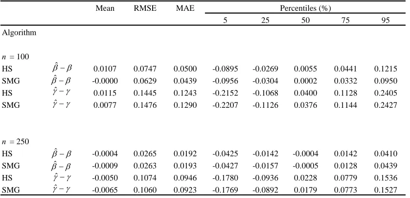
For β =1 and γ =0 the model is estimated using both the HS and SMG algorithms for 1000 replications, using sample sizes of n = 100 and n = 250. To elicit a clear comparison, the HS grid sizes for and are set equal to the number of observations (the same as used by SMG for the threshold 1
). To preserve degrees of freedom, candidates from the grid are only considered when their choice leaves a minimum of five percent of the total observations in each regime. The results are presented in Table 1, reporting the mean, root mean squared error (RMSE), mean absolute error (MAE), and percentiles from the distributions of the estimators.
[Insert Table 1 here]
For 100 observations the performance of both algorithms is quite similar. SMG has a slightly lower RMSE and MAE for , and marginally higher for , although these differences are not statistically significant. The distributions show a roughly equal degree of dispersion; however, HS appears to have a higher bias for both the cointegrating coefficient and the threshold parameter. When n = 250, there are no statistically significant differences in bias or efficiency between the two estimation procedures.
These results generally suggest that both algorithms have a roughly equal degree of efficiency. However, the most striking difference is the number of computations necessary for each replication, which is reported in Table 2.
The grid size for the HS algorithm is the same for each replication, requiring 9,000 models to be estimated when the sample size is 100, and 56,250 when there are 250 observations. Since the SMG algorithm repeats the grid search for the threshold until the likelihood function fails to improve, the number of computations varies for each model. Consequently, the average, minimum, and maximum number of estimations are reported. The average number of estimations is substantially lower for SMG, particularly as the sample size is increased. For 100 observations HS requires nearly thirty times the number of computations, and just over seventy times as many when n is set to 250. In this exercise, the maximum number of grid searches required when applying SMG was eight for both sample sizes. Even at this extreme, SMG is still much quicker than HS. To illustrate the extent of the computational burden, the number of calculations required for the full simulation are also shown. With 250 observations, the HS method required over 56 million, but for SMG it was less than 800,000. This difference is far from trivial to the applied researcher, who will need to run such simulations to acquire accurate p-values to perform hypothesis tests on each individual model they estimate.
These results can be summarised as follows. The newly proposed SMG algorithm is comparable in terms of efficiency to the existing HS method, but appears to have a slightly lower bias in smaller samples. In computational terms, SMG is far quicker. However, the main advantage of SMG is that it can be applied to much larger systems for which HS would be unfeasible. Such an application is now illustrated in the next section.
4. UK term structure of interest rates
R1 = One month LIBOR rate. R3 = Three month LIBOR rate. R6 = Six month LIBOR rate.
The data is monthly, ranging from June 1996 to September 2001 (a total of 100 observations). An example of an unrestricted linear VECM for the three rates is given by
1 1
t t t t
R µ αβ′R− R− u
∆ = + + Γ∆ + (7)
where Rt′ =
[
R1t R3t R6t]
. Applying the Johansen cointegration test to (7), evidence of two cointegrating vectors is found at the five percent significance level. Before proceeding to estimate a corresponding non-linear model, this leaves a number of options available for threshold estimation. For instance, one of the two cointegrating vectors may determine all regime switches, or alternatively each error correction term may respond to separate threshold values (estimating the latter would require a two dimensional grid search over both cointegrating relations). As a compromise, a single threshold value was specified for both error correction terms, with each responding individually. This is reasonable because the spreads R1-R3 and R3-R6 have a roughly equal variance. Experimentation with different possibilities also indicated that this specification produced the most significant non-linear model.The estimated coefficients for the threshold VECM using the SMG algorithm are reported below, with standard errors in parentheses:
1 1 1 1 1
1 1 1 1
1 0.05( 1 0.83 3 0.84) 0.49 ( 1 0.83 3 0.84) (0.09) (0.09) (0.58) (0.15) (0.09) (0.58)
0.29 1 0.09 1
(0.12) (0.19)
t t t t t t
t t t t
R R R d R R
R d R u
− − − −
− −
∆ = − − − − − −
1 1 2 1 1
1 2 1 2
3 0.01( 3 0.78 6 1.23) 0.57 ( 3 0.78 6 1.23) (0.07) (0.04) (0.26) (0.16) (0.04) (0.26)
0.20 3 0.13 3
(0.11) (0.20)
t t t t t t
t t t t
R R R d R R
R d R u
− − − −
− −
∆ = − − − − −
∆ + ∆ +
1 1 2 1 1
1 2 1 3
6 0.08( 3 0.78 6 1.23) 0.68 ( 3 0.78 6 1.23) (0.08) (0.04) (0.26) (0.17) (0.04) (0.26)
0.36 6 0.38 6
(0.11) (0.21)
t t t t t t
t t t t
R R R d R R
R d R u
− − − −
− −
∆ = − − − − − −
∆ − ∆ +
1 1 1 2 1 1
2 2 2
u1 u2 u3
1( 1 0.83 3 0.84 0.17) 1( 3 0.78 6 1.23 0.17) ˆ 0.01 ˆ 0.02 ˆ 0.02
SupLM 4.09 p-value 0.000
t t t t t t
d R R d R R
σ σ σ
− − − −
= − − > = − − >
= = =
= =
The first thing to note is the specification of the regimes. The variables and are activated by the first and second equilibrium relationships respectively, but only when the magnitude of their deviation exceeds the threshold value. This allows the response of the interest rates to change when they are too far from equilibrium, either above or below, so the response is symmetric. The justification for such a specification is based on a simple premise that some agents may have a preference to invest for long periods, whilst others will require shorter commitments. It then follows that a higher rate of return may lead to an aggregate shift towards either long or short term lending, but only if the spread is significantly large. This is very different to the HS application to US term structure, when only large negative deviations induced a change in behaviour.
1t
d d2t
for the six month LIBOR rate. In this case it appears that there is no short-run response at times when disequilibrium is sufficiently large, thereby increasing the relative importance of the error-correction mechanism in the outer regimes. The equilibrium error for the one and three month rates exceeds the threshold in 27% of the sample observations. The deviation of the three and six month rates from equilibrium is slightly more varied, being greater than the estimated threshold for 34% of the time during this period. The SupLM statistic proposed by HS is also presented. An asymptotic p-value is calculated using the fixed regressor boot-strap proposed by Hansen (1996), with 10,000 replications performed in this case. This tests the null hypothesis of a linear model, where for all i, against the above threshold specification. The null is clearly rejected in favour of threshold cointegration.
1i 2i 0
d =d =
5. Conclusion
References
Balke, N.S., and Fomby, T.B. (1997) ‘Threshold cointegration’, International Economic Review, 38, 626-645.
Campbell, J.Y., and Shiller, R.J, (1987) ‘Yield spreads and interest rate movements: a bird’s eye view’, Review of Economic Studies, 58, 495-514.
Davies, R.B. (1977) ‘Hypothesis testing when a nuisance parameter is present only under the alternative’, Biometrika, 74, 33-43.
Hansen, B.E. (1996) ‘Inference when a nuisance parameter is not identified under the null hypothesis’, Econometrica, 64, 413-430.
Hansen, B.E., and Seo, B. (2002) ‘Testing for two-regime threshold cointegration in vector error-correction models’, Journal of Econometrics, 110, 293-318.
Johansen, S. (1988) ‘Statistical analysis of cointegration vectors’ Journal of Economic Dynamics and Control, 12, 231-254.
Tong, H. (1983) Threshold models in non-linear time series analysis. Lecture notes in Statistics, No 21, Heidelberg: Springer.
Table 1
Distribution of estimators
Mean RMSE MAE
5 25 50 75 95
Algorithm
n = 100
HS 0.0107 0.0747 0.0500 -0.0895 -0.0269 0.0055 0.0441 0.1215
SMG -0.0000 0.0629 0.0439 -0.0956 -0.0304 0.0002 0.0332 0.0950
HS 0.0115 0.1445 0.1243 -0.2152 -0.1068 0.0400 0.1128 0.2405
SMG 0.0077 0.1476 0.1290 -0.2207 -0.1126 0.0376 0.1144 0.2427
n = 250
HS -0.0004 0.0265 0.0192 -0.0425 -0.0142 -0.0004 0.0142 0.0410
SMG -0.0009 0.0263 0.0193 -0.0427 -0.0157 -0.0005 0.0128 0.0439
HS -0.0050 0.1074 0.0946 -0.1780 -0.0936 0.0228 0.0779 0.1536
SMG -0.0065 0.1060 0.0923 -0.1769 -0.0892 0.0179 0.0773 0.1527
Percentiles (%)
ˆ
β β−
ˆ
β β−
ˆ
β β−
ˆ
β β−
ˆ
γ γ−
ˆ
γ γ−
ˆ
γ γ−
ˆ
γ γ−
Table 2
Computational requirements of the HS and SMG algorithms
HS SMG(MIN) SMG(AVE) SMG(MAX) HS SMG
Estimations n = 100 9,000 182 305.760 728 9,000,000 305,760
n = 250 56,250 675 796.725 1800 56,250,000 796,725
Grid searches n = 100 1 2 3.360 8 1,000 3,360
n = 250 1 3 3.541 8 1,000 3,541
Simulation Total Required number per replication
1
Note that Hansen and Seo perform a similar simulation exercise. It was, however, felt necessary to produce some new results for their method, not only so that the grid sizes were equivalent, but also so that the HS and SMG algorithms were applied to identical sets of experimental data.
2
[image:17.612.97.505.368.435.2]