Compact microscopy systems with non-conventional optical techniques

i

COMPACT MICROSCOPY SYSTEMS WITH

NON-CONVENTIONAL OPTICAL TECHNIQUES

Tahseen Kamal

A thesis submitted for the degree of Doctor of Philosophy of The Australian National University

March 2018

iii

DECLARATION

This thesis is an original work conducted by me during the period of April 2014 and March 2018 at the Research School of Engineering, Australian National University, Canberra, Australia.

This PhD work has been supervised by Dr. Woei Ming Lee throughout. Certain experimental parts of the works were conducted as group projects with honours students and each of their contribution(s) have been mentioned in detail in the relevant chapters (Chapters 3, 4 and 5) accordingly.

v

vii

ACKNOWLEDGMENTS

I am grateful to my primary supervisor, Dr. Woei Ming Lee, for his constant guidance throughout my PhD which was a roller-coaster journey at times. We worked throughout all the difficulties and were able to accomplish quality research. I would also like to thank the members of the Applied Optics group for their support. Without the group’s support, it would not be possible to stay persistent. I would also like to mention the role Dr. Chuong Nguyen played as associate supervisor. He was there when I needed the most and was always motivating and encouraging when I felt dejected. My other associate supervisor Dr. Thushara Abhayapala is well-known as a mentor and he has proven himself again when I needed his support during my PhD. I also want to thank the Australian Government for PhD scholarship.

During the course of this journey, I received tremendous support from different levels of ANU. Firstly, and most importantly, I want to acknowledge College of Engineering and Computer Science (CECS) Associate Dean (HDR), Dr. Daniel Macdonald, for the financial support I received to continue research. At the same time, he was a good listener to my concerns, who also provided appropriate suggestions. Dr. Henry Gardener, previous CECS Associate Dean (HDR) supported my travel to San Francisco, USA to attend a congress organized by Optical Society of America (OSA), by offering “Carer Career Development Fund” which at the stage PhD students are not eligible to avail from central ANU.

viii

I also want to thank the Computational Imaging group in UC Berkeley, USA for their support during the computational part of my work. Regina Eckert, Zachary Phillips, provided me support whenever we needed. Especially, Dr. Laura Waller, the PI always responded to emails, which was very helpful during the initial days of the work. I want to thank colleagues from different research groups like solar thermal group, nanomaterials, and biomaterials. It is hard to actually mention some names as most of them travelled alongside me. Because of their encouragement I had a successful PhD seminar at the presence of a large audience. There are more people across ANU in other colleges who have been with me if I needed. The PhD journey would not be possible for me without the support of different parents. I am a single mother. Doing a full-time PhD in Engineering was extremely challenging where I needed two pieces of me to support my lab-work and parenting. The parents of the friends of my son, looked out for me constantly.

I want to thank my parents Dr. A. K. M. Kamal Uddin and Mrs. Rehena Begum for believing in me, for allowing me to grow into an independent strong human being, for nurturing me in an educational environment. Without their upbringing I wouldn’t be who I am today. I would also like to mention my brothers Zunaeed and Mr. Muhammad Nasif for being cooperative.

ix

ABSTRACT

This work has been motivated by global efforts to decentralize high performance imaging systems through frugal engineering and expansion of 3D fabrication technologies. Typically, high resolution imaging systems are confined in clinical or laboratory environment due to the limited means of producing optical lenses on the demand.

The use of lenses is an essential mean to achieve high resolution imaging, but conventional optical lenses are made using either polished glass or molded plastics. Both are suited for highly skilled craftsmen or factory level production. In the first part of this work, alternative low-cost lens-making process for generating high quality optical lenses with minimal operator training have been discussed. We evoked the use of liquid droplets to make lenses. This unconventional method relies on interfacial forces to generate curved droplets that if solidified can become convex-shaped lenses. To achieve this, we studied the droplet behaviour (Rayleigh-Plateau phenomenon) before creating a set of 3D printed tools to generate droplets. We measured and characterized the fabrication techniques to ensure reliability in lens fabrication on-demand at high throughput. Compact imaging requires a compact optical system and computing unit. So, in the next part of this work, we engineered a deconstructed microscope system for field-portable imaging.

x

technique that combines the use of synthetic aperture and iterative optimization algorithms, offering increased resolution, at full field-of-view (FOV) and aberration-removal. In using FP techniques, we have shown measurements of optical distortions from different lenses made from droplets only. We also, investigated the limitations of FP in aberration recovery on moldless lenses.

xi

PUBLICATIONS

Journals

1. Tahseen Kamal, Lu Yang, and Woei Ming Lee, “In situ retrieval and correction of aberrations in moldless lenses using Fourier ptychography,” Opt. Express 26, 2708-2719 (2018).

2. Tahseen Kamal, et al., “Design and fabrication of a passive droplet dispenser for portable high resolution imaging system”, Scientific Reports 7, Article number: 41482 (2017).

Conference Proceedings:

1. Tahseen Kamal, Lu Yang, and Woei Ming Lee, "Application of computational optics in moldless lenses," in Imaging and Applied Optics 2017 (3D, AIO, COSI, IS, MATH, pcAOP), OSA Technical Digest (online) (Optical Society of America, 2017), paper JTu5A.14.

2. Tahseen Kamal, Jaden Rubinstein, Rachel Watkins, Zijian Cen, Gary Kong and Woei Ming Lee, “Thimble microscope system” SPIE BioPhotonics Australasia 10013, 1001322-1001322-5 (2016).

3. Tahseen Kamal, Rachel Watkins, Zijian Cen and Woei Ming Lee, “Direct fabrication of silicone lenses with 3D printed parts” SPIE BioPhotonics Australasia, 1001336-1001336-6 (2016).

Letter to the editor:

1. Tahseen Kamal, Xuefei He, Woei Ming Lee, “Reinventing Pocket Microscopy”, InFocus (Proceedings of the Royal Microscopical Society) 37, 41- 43 (2015). News Article:

xiii

TABLE OF CONTENTS

Declaration _________________________________________________________________ iii

Acknowledgments ___________________________________________________________ vii

Abstract ___________________________________________________________________ ix

Publications ________________________________________________________________ xi

Table of contents ___________________________________________________________ xiii

List of Figures _____________________________________________________________ xvii

List of Tables _____________________________________________________________ xxix

Nomenclature ______________________________________________________________ xxx

Chapter 1 Compact high resolution imaging systems __________________________ 1 1.1. Challenges in scientific instrumentation ________________________________ 1

1.2. Evolution of high resolution optical micro-imaging _______________________ 4

1.3. Characteristics of optical imaging systems ______________________________ 9

1.4. Decentralizing high resolution optical microscopes ______________________ 12

1.5. Components of a compact optical microscope system _____________________ 13

1.5.1. Optics ________________________________________________________ 13

1.5.2. Instrumentation ________________________________________________ 13

1.5.3. Computational approaches for compact microscope system ______________ 15

1.6. State of the art of compact imaging systems ____________________________ 15

1.6.1. Lensless ______________________________________________________ 15

1.6.2. Lens-based ____________________________________________________ 17

1.6.3. Lens vs lensless ________________________________________________ 19

1.6.4. Proposed integrated approach _____________________________________ 19

1.7. Thesis organization _______________________________________________ 21

Chapter 2 Droplets for optics _____________________________________________ 23 2.1. Optical materials for lens making ____________________________________ 24

2.1.1. Glass ________________________________________________________ 25

2.1.2. Plastic/polymer ________________________________________________ 26

2.1.3. Transparent Elastomer ___________________________________________ 28

2.2. Study of droplet formation __________________________________________ 30

xiv

2.2.2. Dimensionless entities for flowing liquid and droplet formation ___________ 33

2.2.3. Droplet formation from a falling jet ___________________________________ 36

2.3. Applications of droplets in optics _____________________________________ 37

2.3.1. Lasers ________________________________________________________ 37

2.3.2. Sensors _______________________________________________________ 37

2.3.3. Tunable lenses _________________________________________________ 38

2.4. Manufacturing of optical components _________________________________ 38

2.4.1. Mold-based ____________________________________________________ 38

2.4.2. Moldless ______________________________________________________ 42

2.5. On-demand droplet generation _______________________________________ 44

2.5.1. Active droplet generation _________________________________________ 46

2.5.2. Passive droplet generation ________________________________________ 47

2.6. Chapter Summary _________________________________________________ 49

Chapter 3 Production and performance analysis of moldless lenses _____________ 51 3.1. Passive droplet formation ___________________________________________ 52

3.2. Passive droplet dispenser ___________________________________________ 53

3.2.1. Design and optimization __________________________________________ 53

3.2.3. Drawbacks of the process _________________________________________ 68

3.3. Active droplet dispenser for harvesting moldless elastomer lenses ___________ 69

3.4. Performance analysis of passive droplet lenses __________________________ 71

3.4.1. Wavefront observation using Shack Hartmann wavefront sensor __________ 72

3.4.2. Focal length Optimization ________________________________________ 76

3.4.3. Surface roughness measurement ___________________________________ 77

3.4.4. Imaging performance of the passive droplet lenses _____________________ 77

3.5. Comparison among various moldless lens manufacturing methods ___________ 80

3.6. Contributions ____________________________________________________ 83

3.7. Chapter Summary _________________________________________________ 83

Chapter 4 Integrated imaging system design ________________________________ 85 4.1. Scopes for portable integrated imaging systems __________________________ 86

4.1.1. Applications ___________________________________________________ 86

4.1.2. Challenges ____________________________________________________ 87

4.2. Thimble imaging system ____________________________________________ 88

4.2.1. Design motivation ______________________________________________ 90

4.2.2. Design optimization for thimble parts _______________________________ 91

xv

4.2.4. Choice of optics ________________________________________________ 94

4.2.5. Choice of processor _____________________________________________ 94

4.2.6. Portable, compact system_________________________________________ 96

4.2.7. Imaging performance ____________________________________________ 97

4.3. Portable standalone microscope ______________________________________ 99

4.3.1. Design goals: _________________________________________________ 100

4.3.2. Design optimization: ___________________________________________ 101

4.3.3. Prototype of the microscope: _____________________________________ 101

4.3.4. Imaging performance ___________________________________________ 105

4.4. Compact high resolution, high SBP imaging system _____________________ 106

4.5. Contributions ___________________________________________________ 107

4.6. Chapter Summary ________________________________________________ 108

Chapter 5 Computational techniques based on FOurier Optics ________________ 109 5.1. Simple microscope system ____________________________________________ 110

5.2. Basic Fourier Transform __________________________________________ 111

5.2.1. Numerical Fourier Transform in image processing ____________________ 113

5.2.2. Spatial Filtering _______________________________________________ 116

5.2.3. Optical Fourier Transform _______________________________________ 116

5.2.4. Imaging techniques using Fourier Optics ___________________________ 117

5.3. Inverse Problem _________________________________________________ 119

5.3.1. Phase measurement using optical techniques ________________________ 120

5.3.2. Computational phase retrieval techniques (inverse problem) ____________ 121

5.4. Fourier Ptychographic Microscopy __________________________________ 122

5.4.1. Illumination scheme for Fourier Ptychography _______________________ 123

5.4.2. Forward imaging model in Fourier Ptychography _____________________ 125

5.4.3. Aperture synthesis _____________________________________________ 126

5.5. Proposed experimental work using FP ________________________________ 128

5.6. Proposed reconstruction process ____________________________________ 129

5.7. Sampling criteria for FP reconstruction process ________________________ 132

5.8. Resolution improvement using FP ___________________________________ 132

5.9. Computational aberration correction _________________________________ 133

5.10. Relevant parameters for FP reconstruction ____________________________ 133

5.10.1. Numerical aperture (NA) ________________________________________ 133

5.10.2. System Magnification __________________________________________ 133

5.10.3. LED matrix details _____________________________________________ 134

xvi

5.11. Early results using FP on moldless lenses _____________________________ 134

5.12. Contributions ___________________________________________________ 135

5.13. Chapter Summary ________________________________________________ 136

Chapter 6 Fourier Ptychography on Moldless lenses ________________________ 137 6.1. FP imaging resolution improvement approach __________________________ 137

6.2. Limitations of proposed FP using the proposed imaging setup ________________ 138

6.2.1. Using small aperture LED matrix __________________________________ 139

6.2.2. Raspberry pi camera lens ________________________________________ 139

6.2.3. Initial guess selection ___________________________________________ 140

6.2.4. Reduced spatial coherence _______________________________________ 142

6.3. FP on commercial lenses for proposed system: _________________________ 143

6.3.1. A compound compact system _____________________________________ 143

6.4. FP on moldless elastomer lenses ____________________________________ 144

6.4.1. Single moldless lens system ______________________________________ 145

6.4.2. Compound moldless lens system __________________________________ 146

6.5. Proposed FP on biological samples __________________________________ 147

6.6. Phase retrieval using proposed FP ___________________________________ 149

6.7. Pupil retrieval using proposed FP ____________________________________ 150

6.8. Contributions ___________________________________________________ 151

6.9. Chapter Summary ________________________________________________ 151

Chapter 7 Conclusion __________________________________________________ 153 7.1. Thesis summary ____________________________________________________ 153

7.2. Discussion on moldless lens manufacturing _______________________________ 155

7.3. Discussion on decoupled imaging prototype ___________________________ 156

7.4. Discussion on moldless lens based Fourier Ptychographic Microscopy ______ 156

7.5. Future works ____________________________________________________ 158

Appendix A ______________________________________________________________ 161

Appendix B _______________________________________________________________ 163

xvii

LIST OF FIGURES

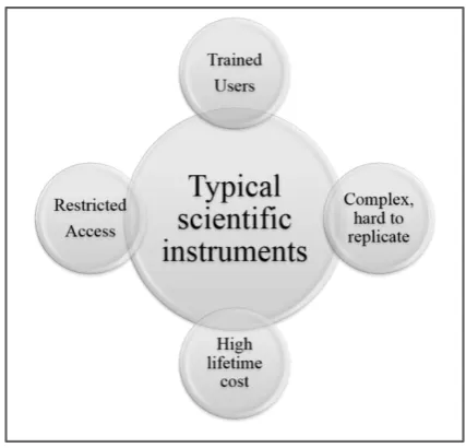
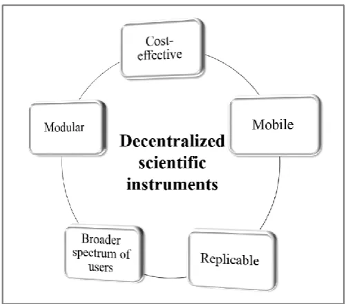
Figure 1:1: Schematic of typical scenario of the use of complex scientific instruments. These instruments are designed and developed in high resource settings, in a laboratory by trained users, which makes them costly, less-accessible and complex... 1 Figure 1:2: Decentralized scientific instrument can be easily transferrable, replicable, and

can broaden research scopes at low-cost. ... 2 Figure 1:3: Decentralized scientific instruments. a) This portable smartphone-based

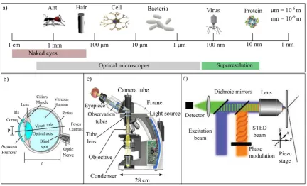
imaging system has been designed to allow microscopic imaging of biological samples [4]. b) MyShake: a smartphone app available for both Apple and Android phones where earthquakes can be detected by using accelerometers of the smartphones. Till date more than 250,000 people have downloaded this app. ... 3 Figure 1:4: Performance of an eye vs optical microscopes to depict the capabilities of

optical microscopes. a) Naked eye is capable of observing as small as 0.1 mm and optical microscopes can resolve as small as 500 nm. b) Structure and optics of an eye. c) A commercial microscope to demonstrate the fixed, rigid, complex structure [22]. d) Stimulated Transmission Emission Depletion (STED) Microscope one kind of super-resolution techniques, that uses a 2nd

source of laser to restrict fluorescence emission within small area and can achieve up to 20 nm [21]. The optical setup has been redrawn from [20] which is fundamental for super-resolution technique. ... 5 Figure 1:5: Different commercial optical microscopes with their a) attributes and b)-c)

the range of options available for microscopic imaging. In b) A commercial microscope that offers both brightfield and phase-contrast imaging [25]. c) A handheld digital microscope which works with a laptop/computer [26]. ... 6 Figure 1:6: Numerical aperture (NA), dimensionless quantity that defines the maximum

angle of light accumulation, is given by, nsin. The value of NA in combination with the wavelength of the light used for imaging, define the lateral (rlateral) and axial (raxial) resolutions. ... 10

Figure 1:7: Space bandwidth products of an imaging system of FOV 784 mm2 _when

different resolutions are achieved. If for the above imaging system, the resolution is a value of 1 mm then the achievable amount of information is 1568 pixels. If the resolution can be improved, keeping the same system to 0.5 mm, the achieved SBP would be 6272 pixels. ... 11 Figure 1:8: Lensless cytometry using lensless digital inline holography that can count and

xviii

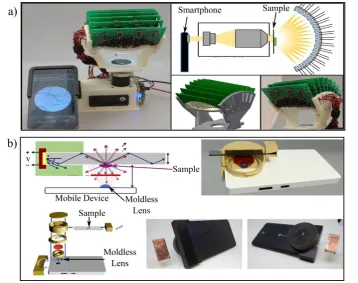
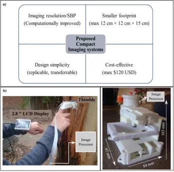
Figure 1:9: State of the art of compact imaging systems using lenses and smartphones. a) Using a cell phone and a hemispherical dome LED array to acquire multiple images of a sample. Also using openCV android based programming which can digitally refocus, acquire phase information [58]. b) A fluorescence microscope using smartphone and inkjet printed moldless lens that can offer autofluorescence, immunofluorescence and fluorescent stains for imaging biological samples in microscopic level [59]. ... 17 Figure 1:10: Proposed integrated high resolution, high SBP imaging system qualities.

Design of the models, credits: Jaden Rubinstein and Michael Petkovic respectively. ... 20 Figure 2:1: Fundamental properties of light. a) Refraction at a curved surface, e.g. a

converging lens. b) Sunlight interacting with a water droplet in atmosphere, rainbow phenomenon, due to Mie scattering. Convexity of a surface is required to offer optical magnification. As, droplets naturally allow bending light at its surface, they offer platform for droplet based optics. ... 23 Figure 2:2: History of grinded and polished optical lenses. A polished lens made by

Antoni van Leeuwenhoek in late 17th _{century, and a handheld microscope to}

attach the lens [69]. ... 24 Figure 2:3: A scenario depicting the complex design process of objective lens made from

glass. a) A typical microscope objective lens with auto correction capabilities. b) Typical spherical glass lens making process, redrawn with permission [81]... 26 Figure 2:4: Sample commercial polymer optics manufactured in industry using injection-molds. Image source: online, used with permission [82]. ... 27 Figure 2:5: Polymerization process of PDMS. a) The monomer of PDMS and the cross-linker/curing agent. b) Bonded PDMS after polymerization. ... 29 Figure 2:6: Formation of a pendant drop. a) A pendant PDMS drop hanging at the tip of

a solid plastic (ABS). b) Different forces acting on the pendant drop to help it retain a convex shape. ... 30 Figure 2:7: Wetting and spreading phenomenon that are important while using a liquid

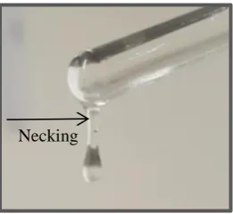
droplet to harvest optical lenses where sufficient. a) Liquid droplet resting on a surface right after deposition. b) After 10 seconds spreading/wetting started to happen. c) Wetting continues as there is no external mechanism to stop the spreading. ... 32 Figure 2:8: A falling liquid jet forming a droplet and a neck is forming. Image has been

acquired in the lab using mixed PDMS. ... 36 Figure 2:9: Pie-chart showing example of injection molding plastic optics manufacturing

xix

Figure 2:10: Compression molding process. The process typically uses two halves of a mold and a piece of solid substrate. The solid substrate is brought to molten stage using high temperature and then placed into the bottom mold. The top mold is then compressed to acquire the desired molded component. ... 40 Figure 2:11: Alternative manufacturing using 3D printing. a) A commercial 3D printer,

up mini printer that can print a volume of 120 mm x 120 mmx 120 mm. b) A comparison showing how injection molded manufacturing and 3D printed are effective in different circumstances [127]. ... 43 Figure 2:12: On-demand droplet generator where the mold substrate has been fabricated

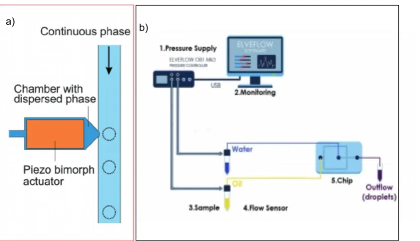
using PDMS and the Norland 65 optical adhesive has been used for the lens material that is a photopolymer [137]. ... 44 Figure 2:13: Different microfluidic geometry used for droplet generation. These two

approaches are the most popular approaches. a) A T junction where a piezo-actuator has been used to inject the dispersed fluid [141]. b) A flow-focusing device where two fluids have been used to create droplets [142]. ... 46 Figure 2:14: Droplet generation in microfluidic devices. The droplets achievable can

range from picoliter to ml (milliliter) [143]. ... 47 Figure 2:15: Pressure driven droplet formation using multiple co-flowing fluid. a)

Squeezing mode of droplet breakup. b) Dripping mode of droplet breakup. ... 48 Figure 3:1:Ppassive droplet dispenser containing three-parts for moldless elastomer lens

manufacturing. Both sideview and top-down view. a) Basin with 5 wells. b) Conic-dropper with 5 conic tips. c) Droplet-holder with 5 holes, each 3 mm diameter. ... 52 Figure 3:2: Product development life cycle (PDLC) for the passive droplet dispenser that

went through iterations to reach to a set of 3D printed tools. ... 54 Figure 3:3: Passive droplet dispenser 3D printed parts printed using an UP mini printer

using ABS as material. a) Three parts, basins, droplet-holder and conic-dropper respectively. b) Clipping mechanism in the design to achieve mechanical stability to avoid perturbation. ... 55 Figure 3:4: Demonstration of the fluidic behaviour when a plastic cone is immersed and

extracted within/from a liquid. a) Immersion, b) Extraction. It is observable that due to capillary forces, the liquid attaches to the tip of the solid cone. 56 Figure 3:5: Post extraction tip of the cone accumulating a volume of liquid PDMS. a)

Schematic showing different forces acting during this observation. b) Experimental observation of the tip of one cone after immersion/extraction. ... 57 Figure 3:6: Jetting when the tip of the cone has been pulled out of the basin. In order to

xx

Figure 3:7: Due to Rayleigh-Plateau instability a liquid jet forms. Then we can observe the dripping process, just the moment before a droplet is getting detached from the flowing liquid jet. ... 58 Figure 3:8: Thin height (~1 mm) droplet holder holding a droplet. a) Schematic depiction

of the process with different forces shown. b) Experimental observation of the retention step. ... 59 Figure 3:9: Three different conic-droppers with varying cone angles, in order to find an

optimum cone angle. a) Flattest tip with cone angle 16.9º. b) Proposed conic-dropper with angle 31.1º and, c) Steepest cone with the angle 58.3º. ... 59 Figure 3:10: Amount of PDMS acquired after immersion/extraction using three different

conic-droppers earlier shown in Figure 3.10. ... 60 Figure 3:11: Two different flowing jets from the tip of two different conic-droppers. a)

Proposed conic-dropper generating a jet of radius 3.088 mm. b) The steep conic-dropper generating a jet of 4.54 mm radius... 61 Figure 3:12: Three different conic-droppers of different angles, generating droplets that

are supposed to be retained at the droplet-holder. a) The dropper with a flat cone is unable to produce a successful droplet. b) Proposed conic-dropper generating a droplet. c) Steep conic-dropper generating liquid with multiple droplets and larger volume that is falling through the hole due to larger bond number. ... 62 Figure 3:13: Droplet-holder with varying heights. a) Wetting/spreading observed at a

droplet-holder of 0.5 mm height. b) Droplet-holder of 0.9 mm height, the proposed design holding a droplet of PDMS. c) A 2.82 mm height droplet-holder generating a droplet of very small convexity. ... 63 Figure 3:14: A lens harvested using the thick droplet-holder showing a thick cylindrical

stem. a) The thick holder used to harvest the lens. b) A shadow image of the lens. c) Schematic showing the thick holder retaining liquid PDMS. d) Due to capillary rise the liquid is pulled up through the thick droplet-holder cylinder. ... 64 Figure 3:15: Wetting/spreading and pinning effect. a) A hole of a droplet-holder without

the proposed barrier. b) Spreading/wetting causes the droplet to disperse as much as possible. c) A hole of the proposed droplet-holder with a droplet retained. A 0.5 mm thick barrier has been shown inset. d) The droplet height reduced by a small margin due to wetting/spreading and inertia caused by surface tension. The spreading has been pinned at the edge of the barrier.. 64 Figure 3:16: Lens making process using the passive droplet dispenser. a) Using a flow

xxi

Figure 3:17: Lenses of various heights produced using the passive droplet approach. The high throughput of this moldless approach also has one added advantage, that the cost per lens does not depend on the number of lenses produced. The lenses cost ~1 cent per lens. ... 68 Figure 3:18: Plano-convex lenses of various diameter and heights manufactured using the

simple active dispenser. ... 69 Figure 3:19: Simple active droplet dispensing plano-convex lens manufacturing process.

a) Process flow chart. b) Graphical depiction of the process. Once the hotplate is preheat (up to 200 ºC), which takes 15 – 20 minutes, and the liquid PDMS is degassed within that time, then the lens-making process takes only a second to provide soft plastic lenses. ... 71 Figure 3:20: Geometric aberrations in optical lenses that can happen due to the

inhomogeneity in refractive indices or irregularity at the surface of the lenses. a) Spherical aberration where different rays do not focus at a single point as expected. b) Wavefront distortion due to the geometric aberrations. ... 72 Figure 3:21: Optical setup for wavefront observation of the passive droplet lenses using

a Shack Hartmann Wavefront Sensor. ... 73 Figure 3:22: Magnitudes of different Zernike orders for the average of a total of 75 passive

droplet lenses compared to the commercial aspheric lens (Thorlabs 352280). ... 74 Figure 3:23: Magnitude of spherical aberration vs focal lengths of 75 passive droplet

lenses. ... 75 Figure 3:24: After filling up the basin wells, if a same conic-dropper has been used for

immersion/extraction of liquid PDMS, with each subsequent immersion/extraction, the amount of liquid at the tip of the cone reduces. The bar graph shows, size of droplet acquired after each dip, alongside the corresponding focal lengths. The numbers 1, 2, and 3 in the horizontal axis refers to number of immersion/extractions. ... 75 Figure 3:25: Focal length optimization. a) Shadow imaging of three different passive

droplet lenses. b) Curve tracing and fitting of the curvatures of the corresponding lenses. c) Calculated vs. experimental focal lengths. ... 76 Figure 3:26: Surface roughness measurements. a) Front surface of a passive droplet

elastomer lens. b) Line plot of the line section shown. c) Front surface of the commercial aspheric lens (Thorlabs 352280). d) Corresponding line plot. 78 Figure 3:27: Transmission based imaging setup for imaging using various droplet lenses.

xxii

Figure 3:28: A negative USAF 1951 resolution target card with groups 0-7 imaged using various passive droplet lenses of various magnifications. Compared with commercial aspheric lens. a) Lens with longest focal length with larger FOV but reduced magnification. Achieved resolution is ~ 30 µm. b) Improved resolution (~ 8.77 µm) but reduced FOV image acquired using another moldless lens. c) The maximum resolution achieved using a short-focal length moldless lens, with a resolution of ~ 3.4 µm. ... 79 Figure 3:29: Tip of an onion root imaged using various passive droplet lenses and

compared with commercial aspheric lens. Lenses used for these data are same as the lenses used in Figure 3.28. ... 80 Figure 3:30: USAF target card images acquired using various moldless lenses. a) Passive

droplet lens. b) Plano-convex lens using simple active approach. c) Thermal printed moldless lens (lens credit: Xu Tao). ... 80 Figure 4:1: Schematic of the modules required for compact high resolution imaging. A

computing platform or processor can offer on-field image processing, optical lenses for allowing high resolution imaging, imaging sensor to capture .... 85 Figure 4:2: Different available imaging options for compact imaging. a) The smallest

camera module in the market Naneye and required components for imaging. Scalebar indicates 1 mm. b) iMX6 board for image processing that works with commercial webcam but there is no display. c) Components of proposed, portable imaging system that includes an image processor, camera and a 2.8-inch (50 mm × 70 mm) touch screen display. ... 87 Figure 4:3: Wearable technologies. a) Synapse smart dress which can detect mood of the

person based on heat sensors. b) UV patch designed by L’oreal to detect UV of the surrounding weather using sensors and a smartphone. c) FingerReader to aid blind people in reading textsd) Thimble imaging system designed for this work... 89 Figure 4:4: Thimble measurement for designing 3D printed thimble support. a) Different

parts of index finger, with measurements of finger data from a population of 5 volunteers. b-c) The thimble design showing mechanical sliding option. 91 Figure 4:5: Thimble imaging prototype and components. i) Printed side-view of the

thimble design prototype with camera and an optical lens attached, ii) proximal brace, iii) front brace, iv) back holder for the raspberry pi camera, v) The 3D model of the raspberry pi camera, vi) front holder of the camera that has the option to support optical lens and illumination, vii) a switch to control illumination, viii) a coin battery to supply power for the illumination, ix, xi) Two neopixel LEDs (5mm × 5mm) with integrated control, and x) A moldless lens for magnification. ... 92 Figure 4:6: Raspberry pi 2 model B specifications. For majority of this research Raspberry

xxiii

Figure 4:7: Portable handheld imaging systems for outdoor imaging. a) Proposed thimble prototype with a camera and optical lens for microscopic imaging (shown inset), all decoupled. b) An image processor that can be handheld for imaging but requires a computer to provide visual feedback. ... 96 Figure 4:8: Reflection based imaging using the thimble prototype. a) Image acquired from

the back of a male redback spider, Latrodectus hasseltii, of body length 3 mm. b) Wing of a common house fly, Musca domestica. ... 97 Figure 4:9: A sea urchin imaged using the thimble imaging system and in-situ image

processing done on raspberry pi. a) A brightfield image of a sea urchin. b) Binarized image, c) Blob area and location detection in terms of pixels. ... 98 Figure 4:10: Transmission based imaging using the thimble imaging system. a) USAF

target card image with achieved resolution of 3.1 µm. b) Parts of a cockroach antenna and bristles. ... 98 Figure 4:11: Design goals set for the project on “Standalone microscope”. The design

goals primarily involved, use of 3D printed parts to ensure open-source access of the parts, then cost and compactness. ... 100 Figure 4:12: Illumination options for the proposed prototype. A single white LED offers

simplicity and single brightfield imaging. Whereas, an 8×8 RGB LED matrix offers different angular illumination and spectral imaging options. ... 101 Figure 4:13: Three parts for the standalone microscope. i) A cover to hold the 2.8-inch

LCD display, ii) Front cover for the raspberry pi processor, iii) Back cover for the processor. ... 102 Figure 4:14: Support for optical alignment between camera and objective lens. a) Front

cover for raspberry pi camera. b) Back cover for the raspberry pi camera/CMOS. ... 102 Figure 4:15: X-Y translational stage design and demonstration. a) Mount, bottom-up

view. b) Mount, top-down view, c) x-y stage, d) the mount and the stage attached, e) The sample holder, f) Demonstration of the x-y stage with a microscope glass slide. ... 103 Figure 4:16: Z-axis (the axis normal to the x-y axes) alignment of the microscope for

CMOS height adjustment. a) A pillar that provides the backbone support for the microscope with a helical engraving. b) A collar with clips and a hemispherical anchor, that allows for the collar to rotate and move up-down for z-alignment. c) Collar attached to the helical engraving, rotating left-right. d) Rotation causes the collar to move upwards. e) Top mount for the z-alignment control for stability attached with the back cover for the CMOS (bottom-up view). f) Collar and the mount attached. ... 104 Figure 4:17: The proposed compact standalone microscope. a) The 3D model. b) The

xxiv

Figure 4:18: The properties of the 3D printed standalone microscope that has been achieved from the project... 106 Figure 4:19: Lung cancer tissue sample imaged using the proposed standalone

microscope and a cropped region shown in the red rectangle. ... 107 Figure 5:1: A simple imaging system. The mathematical model applicable for the

majority of the thesis. In an imaging system we have an illumination plane to provide illumination, sample or object plane – sample of interest, the lens aperture plane which can be considered equivalent to the pupil plane. Finally, the image forms on the image plane. Redrawn from similar thesis [166]. 109 Figure 5:2: Different types of transmission-based illumination used for microscopic

imaging. a) Köhler illumination is most commonly used brightfield microscope system used with incoherent illumination such as a bulb. b) If a disk is placed to block certain central portion of the light coming from the source and only the scattered light from the edges are collected by the sensor then that arrangement is known as dark-field illumination. Redrawn from similar thesis [166]. ... 110 Figure 5:3: 2D sinusoidal gratings created in MATLAB to demonstrate concepts of spatial

frequency, phase shift. In (a) we can see a grating corresponding to the equation, y110sin(2 3 ) x , whereas in (b) we can see a 2D grating with a 45º shift. (c) demonstrates the phase shift with the use of 1D line plots. ... 112 Figure 5:4: When light as a wave propagates through different samples the resulting

waves alter differently depending on the sample. The amplitude of the incoming light wave changes enough through amplitude objects (ΔA) which can be detected by a detector due to sufficient contrast. However, for phase objects the amplitude does not change enough to create enough contrast. For these the phase delay information (Δφ) is of importance to create contrast [66]... 113 Figure 5:5: (a) An intensity image with vertical gratings. (b) Another intensity image

where the gratings have certain angular displacements. (c) The Fourier transform of the image present in Figure 5.4(a). The three bright dots in the Fourier image represents that there is a single spatial frequency present in the original image. (d) The Fourier transform of the image shown in (b). The diagonal representation of the dots in the Fourier image represents the corresponding angular representation of the grating in (b). ... 114 Figure 5:6: Two images and their corresponding Fourier Transforms. (a) A grayscale

xxv

Figure 5:7: (a) A grayscale image [169]. (b) The 2D Fourier Transform of the image. (c) Some random filters blocking some high frequencies. (d) The corresponding image after applying the low pass filter which is evident to be blurred after some high frequencies are blocked. (e) A filter that is blocking the low frequencies. (f) The image corresponding to the high pass filter where it is evident the low frequencies are blocked, and the high frequencies are representing the edges. ... 117 Figure 5:8: The concept of Fourier transform using a lens is illustrated here. When plane

waves are diffracted off an object at 1-focal distance of the lens, an image is created at the conjugate focal plane of the lens, which is labelled as image plane. The image plane shows three points because of the transparency placed at the input image plane. ... 118 Figure 5:9: Simple schematic depicting forward vs inverse problem. If we consider the

image acquired by the lens shown in Figure 5.10, then it is noticeable that the imaging system recorded only intensity information. From this intensity information using Fourier optics and iterative algorithms we can retrieve phase, which is the inverse problem for imaging systems. ... 119 Figure 5:10: A diatom imaged using a brightfield microscope (left) and with a phase plate

(right). Oldest photomicrograph recorded by Zernike in 1932 [175]. ... 120 Figure 5:11: Original error-reduction algorithm used by Gerchberg-Saxton for phase

retrieval from intensity images only [177]. ... 121 Figure 5:12: Iterative algorithm for optimization of object and pupil using Fourier

Ptychography [12]. In this work they have used Newton’s 2nd _order

optimization approach to iteratively improve the sample spectrum (O) and in parallel retrieve the pupil (P). Our proposed work uses a modified version of this algorithm. ... 122 Figure 5:13: Schematic of experimental setup for Fourier Ptychography. An LED matrix

(24 × 24 size with a total of 576 LEDs and the index of the centre LED being 276) is used to replace the illumination of a microscope to acquire multiple images of the sample. ... 123 Figure 5:14: Shifting illumination using an LED matrix for Fourier Ptychographic

Microscopic technique. a) A simple imaging setup shown different planes as discussed in section 5.1. Convolution of pupil wavefront and sample wavefront is acquired at the sensor. b) Shows the complete Fourier spectrum achievable through shifting illumination [166]. The NAillumination is achieved

xxvi

Figure 5:15: Shifted illumination capturing larger cone of light in the imaging system using the same lens. A typical microscope with an objective lens of aperture

sin

NAn  provides can capture only the red cone of rays emerging at half of

θ. If the illumination is shifted it is also possible to capture the green cone of rays. FP uses q different LEDs to capture q unique images of the sample. From the set of q images FP can computationally reconstruct an image with larger synthetic NA [166]. ... 127 Figure 5:16: Proposed experimental setup for implementing Fourier Ptychography. This

whole setup requires 10 cm × 10 cm × 15 cm, thus offers high quality imaging (post-reconstruction) in compact form. ... 128 Figure 5:17: Simple process flow diagram of how FP reconstruction works. The process

requires multiple sampling parameters to be set based on the imaging system. Optimization is achieved through iterative reconstructions on a selected region of interest, as FP works base on local optimization. ... 129 Figure 5:18: Proposed Fourier Ptychography reconstruction algorithm [181]. The FP

process works by moving back and forth between spatial and Fourier domains. Here one iteration of the whole process has been demonstrated with the use of Fourier and spatial spectrum. ... 130 Figure 5:19: Performance of FP on different imaging systems using moldless lenses. We

used one raw image taken using center LED and have demonstrated performance on a selected region. ... 135 Figure 6:1: Demonstration of performance of FP on a robust laboratory based system on

a blood smear dataset [188]. a1-c1) The amplitude of the recovered object and pupil after reconstruction. a2-c2) The phase of the recovered object and pupil. The pupil wavefront has been shown in c2 with the Zernike distribution of the retrieved aberrations can be seen in (d). ... 138 Figure 6:2: Images acquired using a commercial aspheric lens cascaded with an objective

5x. The left image was taken when the pi camera lens was present. The right image was captured removing the pi camera lens of the system. ... 140 Figure 6:3: Impact of choosing different initial guesses on an ROI for reconstruction on

data acquired using a commercial aspheric lens. a) Full FOV raw image using center LED. b) Cropped raw image from the ROI shown in green. c)-e) Reconstruction results for initial guesses a-c respectively. The variations in the reconstruction results provide us with the idea that FP works on local optimization and we need to tune the initial guess for each ROI. ... 140 Figure 6:4: Variation in initial guess for a moldless lens based imaging setup. The

xxvii

Figure 6:5: (Left) Adafruit RGB LED matrix without a cover. (Right) ICstation LED matrix within a package. We used 9 of these LED matrices to achieve a larger 24×24 LED matrix. ... 142 Figure 6:6: Resolution improvement limitation of the proposed high resolution imaging

system using non-conventional optical techniques (Fourier Ptychography and moldless lenses). (Left)- raw image. (Right)-reconstructed image. The green square demonstrates the achieved resolution (smallest resolvable distance) after processing, which is, group 7 element 1, is 3.91 µm based on standard values. The red rectangle highlight resolutions that were not achieved. If the expected resolution of 0.61 µm has been achieved other elements of group 7 would be resolved too. ... 143 Figure 6:7: Performance of FP on a compact imaging system using commercial lenses. a)

Schematic of the optical imaging setup. b) A raw image acquired using the centre LED, which is incident on the optical axis. c) The full FOV reconstructed image. d) Analysis of performance demonstrating pixel density improvement and contrast improvement. ... 144 Figure 6:8: Performance of FP on moldless lens based simple imaging system. For this

setup we used a moldless lens of focal length = 12 mm. a) Raw image using centre LED. b) Full FOV reconstructed image. c) Performance analysis of the reconstructed image. The cropped image is group 7 element 1 which in the raw image contains only 34×34 pixels whereas the reconstructed image contains 3 folds higher density. The pixel sizes can be apparently seen to have improved also. The contrast improvement has been demonstrated using line plots. The achieved resolution is 3.91 µm. ... 145 Figure 6:9: Performance of FP on moldless lens based compound imaging system. For

this setup we used a pair of moldless lenses of focal length = 16 and 17 mm, respectively. a) Raw image using centre LED. b) Full FOV reconstructed image. c) Performance analysis of the reconstructed image. The cropped image is group 7 element 3 which in the raw image contains only 47×47 pixels whereas the reconstructed image contains 2 folds higher density. The pixel sizes can be apparently seen to have improved also. The contrast improvement has been demonstrated using line plots. The achieved resolution is 3.1 µm. ... 147 Figure 6:10: Infected red blood cells imaged using a single moldless lens-based imaging

xxviii

Figure 6:11: Demonstration of effectiveness of pre-processing as discussed in [189]. By acquiring multiple images of the sensor at different exposure over a certain period of time, and then subtracting the dark current data as a measure for background subtraction, the pre-processing has been achieved. a) Cropped raw image showing groups 6-7. b) FP reconstruction without using the dark current noise subtraction. c) FP reconstruction with the dark current based pre-processing steps. The performance of c) is better in terms of contrast and structural similarity. ... 148 Figure 6:12: Phase retrieval using proposed compact imaging system and Fourier

Ptychography. a) Wide FOV phase retrieved for the data acquired using an aspheric lens cascaded with objective 5x. There is noise in the phase due to the negative USAF target card generating black background (0 grey values in the matrix). b) Phase retrieved for a red blood cell. Data shown in Figure 6.7. ... 149 Figure 6:13: Pupil retrieval using FP on moldless lenses for dataset shown in Figure 6.7.

a) Here, we have summarized the retrieved pupil on 5 different locations for the dataset shown in Figure 6.7. The off-axis aberrations appear to be higher than the on-axis aberration as expected. b) The Zernike decomposition of the pupil aberrations for modes up to 40. ... 150 Figure 6:14: Retrieved pupil for dataset shown in Figure 6.8, compound imaging system.

a) We have summarized the retrieved pupil on 5 different locations for the dataset shown in Figure 6.9. Like the Figure 6.11, the off-axis aberrations appear to be higher than the on-axis aberration as expected. b) The Zernike decomposition of the pupil aberrations for modes up to 40... 151 Figure 7:1: Portable lens-maker that can print a range of moldless lenses using in-situ

heating element. This 3D printed prototype has been developed by Xu Tao, 4th _{year honours student. ... 155}

Figure 7:2: Peak-to-valley cumulative aberrations acquired from the proposed composed imaging system using various lenses. It is observable that the imaging system where a pair of moldless lenses was used for imaging (Figure 6.6) demonstrated higher magnitude of aberrations. Accordingly, the compound commercial objective 5x lens demonstrated the least aberrations. ... 157 Figure 7:3: Microfluidic channel observation using a moldless lens and the proposed

xxix

LIST OF TABLES

Table 1-1: Attributes of the example microscopic units shown in Figure 1.4. ... 7 Table 2-1: Dimensionless quantities for mixed PDMS liquid flowing in air. ... 35 Table 3-1: Lens parameters corresponding to the lenses used for imaging of the samples

xxx

NOMENCLATURE

Name Symbol

Computer Aided Design CAD

Density ρ

Surface tension γ

Viscosity µ

Numerical Aperture NA

Refractive Index n

Space Bandwidth Product SBP

Signal-to-Noise ratio SNR

Charged Coupled Device (Sensor) CCD

Complementary Metal Oxide Semiconductor (Sensor) CMOS

Polydimethylsiloxane PDMS

1

CHAPTER 1

COMPACT HIGH RESOLUTION IMAGING SYSTEMS

In this chapter we will discuss the overarching problems and current approaches to achieve high quality scientific instruments at low-resource settings, especially, compact, high resolution, imaging systems. Typical optical microscopes are based on laboratories and possess certain limitations. We will discuss how these problems can be tackled using novel, non-conventional approaches. Our discussions will be restricted to non-ionising imaging systems, i.e. optics and Fourier optics approaches. The novel approaches we have proposed in this thesis involve use of moldless droplet lenses, 3D printed architecture to offer decoupled, decentralized imaging systems and use of computational Fourier optics to offer high resolution imaging using the proposed systems.

Figure 1:1: Schematic of typical scenario of the use of complex scientific instruments. These instruments are designed and developed in high resource settings, in a laboratory by trained users, which makes them costly, less-accessible and complex.

1.1. Challenges in scientific instrumentation

2

applications in environments with low-resource settings. If we consider health industry as an example, a patient needing healthcare needs to access a facility, such as a hospital or diagnostic centre, waiting for a physician to provide results is the existing picture of accessible care and service. Point of care, point of procedure healthcare is an ongoing research area that tends to offer real-time healthcare where needed, e.g. relocating medical imaging from hospital to bedside of the patients [1]. Alternatively, if we consider an optical laboratory providing microscope supports for high quality imaging or a biomedical engineering laboratory where researchers are involved to observe complex biological events, typically require centralized, laboratory-based instruments [2]. It is very common that the building blocks of these complex instruments are available from only a few vendors and the production process is hard to replicate due to the cost and complexity [3]. Moreover, factors like, maintenance [3], transportation of these complex instruments add to the overall lifetime cost. Figure 1.1 articulates the idea of traditional use of complex, high performing scientific instruments.

3

Decentralization of the scientific instruments is an attractive avenue for science to leave the laboratory – especially if high quality results are ensured. That can be achieved,

• by allowing the option to relocate them into different work environments (in laboratory or at a low-resource setting outside laboratory),

• by providing access to broader spectrum of users (specialists to non-specialists) with proper to minimal training,

• with promises to be cost-effective, and

• with provisions for replicability at minimal cost.

Figure 1:3: Decentralized scientific instruments. a) This portable smartphone-based imaging system has been designed to allow microscopic imaging of biological samples [4]. b) MyShake: a smartphone app available for both Apple and Android phones where earthquakes can be detected by using accelerometers of the smartphones. Till date more than 250,000 people have downloaded this app.

4

shared across the globe, using web or open-source designs like CAD. The use of the high performing scientific instruments by more users, does allow more research and promise scientific advancement.

However, in this work we confine our discussions into high quality imaging systems. As the imaging systems that we are offering have the capabilities to observe smaller samples, in the microscopic resolution, we will discuss about optical microscopes in the following sections. The use of simplistic optics [8], modular housing using 3D printed building blocks [9] and consumer driven electronics such as raspberry pi [10]– has made it possible for decentralization to provide high quality portable imaging systems – at low-cost, for broader spectrum of users. The use of computational reconstruction ensures improved signal – to – noise (SNR) ratio by deploying digital refocusing [11], background noise reduction [12], etc. - at no additional financial cost, but with sacrifice of computational cost.

1.2. Evolution of high resolution optical micro-imaging

Since early 19th _{century optical imaging through high grade optical lenses have}

5

imaging system. A commercial brightfield microscope system has been shown in Figure 1.4(c). The idea of super-resolution has evolved recently where typical resolution limit of optical microscope can be overcome to achieve even ~10 nm resolution [20, 21]. One example of laser-scanning type super-resolution microscope is the Stimulated Transmission Emission Depletion (STED) fluorescence microscope that uses 2 sources of laser to generate a narrow, focused beam by selectively deactivating certain fluorophores that can achieve lower resolution than typical confocal microscopes. Schematic of a typical STED setup has been shown in Figure 1.4(d). There are other types of fluorescence-based super-resolution microscopes that can be found in literature [21].

Figure 1:4: Performance of an eye vs optical microscopes to depict the capabilities of optical microscopes. a) Naked eye is capable of observing as small as 0.1 mm and optical microscopes can resolve as small as 500 nm. b) Structure and optics of an eye. c) A commercial microscope to demonstrate the fixed, rigid, complex structure [22]. d) Stimulated Transmission Emission Depletion (STED) Microscope one kind of super-resolution techniques, that uses a 2nd _{source of}

laser to restrict fluorescence emission within small area and can achieve up to 20 nm [21]. The optical setup has been redrawn from [20] which is fundamental for super-resolution technique.

6

resolution has been discussed by Abbe in 1873 [23], which is defined by, the wavelength (λ) of the radiation, the diameter (d) of the aperture and the focal length (f) of the lens.

For example, for fixed optical lenses, the visible-broadband light sources (390 nm, violet – 680 nm, red) provide, achievable resolution from 200 nm to 400 nm. The physical attributes that limit the performances of optical microscopes have been elaborated in section 1.3. A major limitation in optical imaging is the size of the imaging aperture of the lenses used. Computational optical approaches have been emerged to overcome these limitations [11, 12, 24].

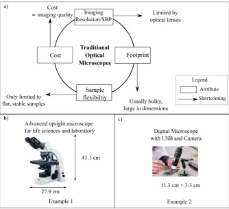
Figure 1:5: Different commercial optical microscopes with their a) attributes and b)-c) the range of options available for microscopic imaging. In b) A commercial microscope that offers both brightfield and phase-contrast imaging [25]. c) A handheld digital microscope which works with a laptop/computer [26].

7

diagnostics) [27]. With higher power lenses, it has become possible to track sub-cellular features (organelles), and for high energy photons, commonly used in semiconductor industry (wafer). Light is non-invasive in nature that is highly suitable for in-vivo events especially in biological systems. However, the footprint and the overall complexity of the optical microscopes for high power imaging grew exponentially. The upward drive in cost of the microscopes coupled with increasing educational and research institutions, has created a vibrant economic market for optical microscopes, where the global demand is expected to reach over $2.58 billion USD by 2022 [28].

Table 1-1: Attributes of the example microscopic units shown in Figure 1.5.

Another feature of the optical microscopes is the types of imaging geometry they cater to. They require flat samples rested on a horizontal plane, stained/labelled or sectioned thin on a microscope glass slide. For ophthalmology patients need to visit a facility where the imaging devices are used by specialized optometrists/ ophthalmologists. Due to many design and accessibility constraints, it is always presumed that the commercial microscopes are better suited for laboratories and trained operators. While the overall cost of a scientific imaging microscope unit remains out of reach for the masses, its inflexible design limits its widespread use.

8

to different live-imaging subjects or subjects located in the field, i.e., insects, leaves, fungi etc. Pathological studies of living samples are very crucial for understanding disease progression (e.g. studying extra-cellular matrix mechanics has proven to be helpful for diagnosing diseases at early stage [30]). This is especially important for low-resource areas where clinical imaging has been hindered by medical costs of traditional microscopes due to their rigid design structure or portability. Figure 1.5 is a comprehensive summary of the existing optical microscopes, the attributes, and the limitations they possess. Cost usually is proportional to the imaging quality/resolution expected from an optical microscope. The footprint, size of these traditional microscopes is large which restricts these devices in a laboratory environment. Also, the microscopes can usually image samples on a stage, which is along the optical axis of the system.

Consumer electronics motivated by global communications networks has powered new innovative portable computing and imaging platforms [1]. While existing miniature optical components have shown to be compatible with the portable computing and imaging systems to create microscopes, the support network for microscopic imaging for broad research in education, academia and industry is lacking a decentralisation model to meet the global demand. The above discussion is to enlighten the fact that existing optical microscopes with fixed optical alignment are limited, i) by the way they are structured, ii) by the fixed, rigid size of the optical lenses, iii) by the footprint of the microscopes, and iv) for lots of scenarios, by the cost.

9

flexibility for the end users to change the overall design for their own uses. For example, an imaging system that can change from a high-end microscope imaging to dermatology requires different imaging and computational specifications. Here, we attempt to lay the foundation for decentralized models for high resolution imaging. To accomplish these ambitious goals, we would require non-conventional approaches in optical lenses fabrication and computational optics techniques. The different parameters that we have aimed to satisfy through this research are:

i) de-coupled imaging unit from computing unit, ii) portable and reconfigurable,

iii) Overcoming limits of optical resolution and SBP,

iv) In-situ removal of optical aberrations of miniature lenses and v) Affordable cost and sustainable fabrication approaches.

1.3. Characteristics of optical imaging systems

Optics has been a cornerstone in imaging wide range of samples. It was only until Abbe where the full formalisation of imaging resolution was established. A key notion from Abbe is that all optical systems (including microscopes) are bound by the wavelength and physical aperture of the lenses through the relationship known as numerical aperture (N.A.). Before discussing the limitations of any optical microscopes, it is important to discuss about certain attributes of microscopes.

Numerical aperture (NA): is a dimensionless quantity that describes the amount of

10

Resolution: Lateral resolution, r_lateral, is defined by smallest distance between two

elements that can be separated from the image,

2 lateral r

NA 

  , where λ is the wavelength

of the light and NA is the numerical aperture, as defined by Abbe [23]. The axial resolution is given by, r_axial 2 ₂

NA



  which defines the depth of focus achievable from the imaging

system. The different resolutions have also been shown in Figure 1.6.

Figure 1:6: Numerical aperture (NA), dimensionless quantity that defines the maximum angle of light accumulation, is given by, nsin. The value of NA in combination with the wavelength of the light used for imaging, define the lateral (rlateral) and axial (raxial) resolutions.

Space bandwidth product (SBP): Another imaging parameter that is the amount of

sampling points for the entire field of view of a lens. In digital optical imaging, an array of densely packed photodetector arranged in a grid format is used to sample a given imaging field. This can be quantified by the use of space-bandwidth product (SBP), SBP is a scalable, dimensionless quantity that usually expresses the amount of information transmitted by the microscopic system that is the total number of resolvable points over a given FOV (often expressed in terms of number of pixels). And is given by the equation,

2

0.5_lateral

FOV SBP

r

 , where rlateral is the lateral resolution.

11

magnification and NA. In other words, SBP is the measure of maximum pixels required over a full FOV with maximum achievable resolution. A conceptual model of SBP has been shown in Figure 1.7, where 2 different achievable resolutions have been shown and that SBP is scalable with lateral resolution and/or FOV.

Figure 1:7: Space bandwidth products of an imaging system of FOV 784 mm2 _{when different}

resolutions are achieved. If for the above imaging system, the resolution is a value of 1 mm then the achievable amount of information is 1568 pixels. If the resolution can be improved, keeping the same system to 0.5 mm, the achieved SBP would be 6272 pixels.

All the above parameters are crucial attributes to generate a high quality image from an imaging system especially in optical microscopy system. Another limitation of lenses is that light can be easily distorted due to refractive index inhomogeneity. Ideally a perfect lens would be able to focus all rays on a single spot, but all lenses are polished to a certain degree of accuracy and inherently possess some amount of optical aberrations. This is especially difficult in smaller lenses where the mechanical fabrication steps require even higher precision. To fully achieve the maximum imaging performance of an imaging system, it would require removal of all the distortions that is practically difficult to achieve for the masses [34].

12

emerging method to overcome many of these physical limitations of existing optical systems [11, 35]. The idea of computational microscopes is rooted in Fourier optics, which allow light to be defined in terms of a complex quantity. It is with the computational optics that optical phase can be numerically retrieved through phase retrieval techniques (inverse problems). Both Fourier optics and phase retrieval will be elaborated in Chapter 5.

1.4. Decentralizing high resolution optical microscopes

13

1.5. Components of a compact optical microscope system

The breakdown of the components that are usually required to acquire high quality optical microscopes using consumer electronics has been discussed in the following subsections.

1.5.1. Optics

Traditionally, all microscope systems require optical lenses for imaging. Hence, the choice of lenses is crucial. Optical lenses have evolved and improved over the last few centuries. In current world a lens can be a singlet lens or a compound microscope objective lens with minimum 20 singlet lenses placed deliberately in certain way to provide high quality imaging performance. However, objective lenses with higher NA and higher magnification capabilities are larger and heavier in physical dimensions, and also costlier.

These compound lenses are bulky which makes them unattractive for low-cost, high portable imaging systems. Lenses with larger numerical aperture will allow more light to be collected by the system and thus improve resolution. But that will increase the aberrations. Moreover, for smaller compact imaging systems increasing the physical dimension of the lenses is unintended. Additionally, decentralised manufacturing of lenses using existing approaches for use in low-resource setting does not yet exist. That gave rise to the idea that we have discussed in this thesis.

1.5.2. Instrumentation

To develop optical imaging systems, we need other supporting instruments to acquire high quality images. Depending on the imaging needs the requirement of the instrumentations could vary. The components to acquire compact high-quality microscope images are discussed in the following subsections.

Electronics: Electronics has become integrated part of our daily life. Imaging systems

14

tomography imaging system, different electronics like logarithmic amplifier, field programmable gate arrays (FPGA) or RMS voltmeters could be used [44]. In modern microscopy, the purpose of electronics can be (and are not limited to), i) providing illumination with automatic control [45], ii) mechanical control actuation (e.g. sample stage) using a microcontroller [46], iii) in situ processing of the images to achieve information or improved imaging quality using an image processor [47, 48]. A simple and quality example could be the use of smartphone-based imaging systems as they are capable of providing on-spot processing with an imaging sensor available. Alternatively, another example of a processor can be raspberry pi, that is low-cost ($35 USD), that can be used for mechanical control of multiple devices such as, LED, motors, camera and also for in-situ image processing [48].

Opto-electronics (imaging sensor): Handheld microscopes developed in as early as

17th _{century are compound microscopes where the naked eyes are used to observe the}

15

CCDs are being replaced by CMOS because they provide high speed and high functionality but at the cost of noise and sensitivity. A raspberry pi camera is an example of miniaturization where a recorded image with 5 megapixels information in an area of 3.76 mm × 2.74 mm, with pixel resolution of 1.4 µm [8].

1.5.3. Computational approaches for compact microscope system

Modern optical instruments are increasingly becoming digitised through CMOS, spatial light modulator and sensors. This means that many concepts in Fourier optics can now be undertaken with relative ease. Computational imaging is a branch of optics that makes use of the information theory to acquire high dimensional information that has not been originally offered by the system [50] which in turn improves the quality of the resulting/reconstructed image through computational approaches [11]. A compact imaging system that leverages computational approaches will increase the imaging performance drastically. Using computational approaches, the NA and SBP of the imaging systems can be improved [11, 37].

1.6. State of the art of compact imaging systems

There are emerging technologies that focus on developing compact imaging systems to serve biometric security, mobile health [51, 52], or in-situ automatic cell identifier [53]. The different approaches for compact high resolution imaging systems can be broadly categorized in two categories, a) lensless and b) lens-based [37].

1.6.1. Lensless