Numerical solution of differential equations using multiquadric radial basis function networks

(1)

Numerical Solution of Dierential Equations

using Multiquadric Radial Basis Function

Networks

Nam Mai-Duy and Thanh Tran-Cong

Faculty of Engineering and Surveying,

University of Southern Queensland, Toowoomba, QLD 4350, Australia

Contributed Article submitted to

Neural Networks

, August 1999,

revised 9 October 2000

Acknowledgements: This work is supported by a Special USQ Research Grant (Grant No 179-310) to Thanh Tran-Cong. Nam Mai-Duy is supported by a USQ scholarship. This support is gratefully acknowledged. The authors would

like to thank the referees sincerely for their helpful suggestion to improve the original manuscript.

Running title: Solving DEs using MQ RBFNs

Corresponding author: Telephone +61 7 46312539, Fax +61 7 46 312526, E-mail [email protected]

(2)

Solving DEs using MQ RBFNs 2 Numerical Solution of Dierential Equations using Multiquadric Radial Basis Function Networks

Abstract

. This paper presents mesh-free procedures for solving linear dierential equations (ODEs and elliptic PDEs) based on Multiquadric (MQ) Radial Basis Function Networks (RBFNs). Based on our study of approximation of function and its derivatives using RBFNs that was reported in an earlier paper (Mai-Duy and Tran-Cong, 1999), new RBFN approximation procedures are developed in this paper for solving DEs, which can also be classied into two types: a direct (DRBFN) and an indirect (IRBFN) RBFN procedure. In the present procedures the width of the RBFs is the only adjustable parameter according toa(i) =d(i),

whered(i) is the distance from the ith centre to the nearest centre. The IRBFN

method is more accuarte than the DRBFN one and experience so far shows that can be chosen in the range 7 10 for the former. Dierent combinations of RBF centres and collocation points (uniformly and randomly distributed) are tested on both regularly and irregularly shaped domains. The results for a 1D Poisson's equation show that the DRBFN and the IRBFN procedures achieve a norm of error of at leastO(1:0e;4) and O(1:0e;8), respectively, with a centre

density of 50. Similarly, the results for a 2D Poisson's equation show that the DRBFN and the IRBFN procedures achieve a norm of error of at leastO(1:0e;3)

andO(1:0e;6), respectively, with a centre density of 1212.

Keywords: Radial basis function networks, multiquadric function, global

(3)

Solving DEs using MQ RBFNs 3 Notations

superscripts denote elements of a set of neurons or collocation points subscripts denote scalar components of a vector

n number of collocation points m number of neurons

x independent variables

ue exact solution

u approximant of the exact solution ue

uij:::l partial derivative of function u with respect to xixj:::xl

ui approximate functionu obtained by integrating uii

g radial basis function

h basis function obtained by dierentiatingg h basis function obtained by dierentiatingh H basis function obtained by integrating g

H basis function obtained by integrating H w weight of basis function

a width of basis function

r radius from the centre located at the neuron under consideration

c \spatial position" of the neuron (centre) k:k Euclidean norm

scalar factor

(4)

Solving DEs using MQ RBFNs 4

1 Introduction

Many problems in science and engineering are reduced to a set of dierential equations (DEs) through the process of mathematicalmodelling. Although model equations based on established physical laws may be constructed, analytical tools are frequently inadequate for the purpose of obtaining their closed form solution and usually numericalmethods must be resorted to. Principal numerical methods available for solving DEs include the Finite Dierence Method (FDM) (cf. Smith, 1978), the Finite Element Method (FEM) (cf. Cook et al, 1989 Hughes, 1987 Zienkiewicz and Taylor, 1991), the Finite Volume Method (FVM) (cf. Patankar, 1980) and the Boundary Element Method (BEM) (cf. Brebbia et al, 1984). These methods generally require some discretisation of the domain into a num-ber of nite elements (FEs), which is not a straightforward task. In contrast to FE-type approximation, neural networks can be considered as approximation schemes where the input data for the design of a network consists of only a set of unstructured discrete data points. Thus an application of neural networks for solving DEs can be regarded as a mesh-free numerical method. It has been proved that radial basis function networks (RBFNs) with one hidden layer are capable of universal approximation (Park and Sandberg, 1993). For problems of interpolation and approximation of scattered data, there is a body of evidence to indicate that the multiquadric function (MQ) yields more accurate results in comparison with other radial basis functions (Franke, 1982 Powell, 1988 Haykin, 1999, p265). Although it is not proved even experimentally in the present work that MQ function would result in superior accuracy for solving DEs, the MQ function is used to study the solution of DEs in this paper based on the above observation because the main aim of the present work is to demonstrate the pro-cedure for solving DEs rather than the study of the property of the kernels. It is important to note that the accuracy of the RBFN solution is inuenced by a parameter which is usually referred to as the width of basis function. The value of this parameter controls the shape of the basis function or the response of the associated neuron. In the case of learning network, the width parameter measures the degree to which excited neurons in the vicinity of the winning neuron partic-ipate in the learning process (Haykin, 1999). Similarly, in the case of functional approximation, the width parameter of a basis function (centre) controls its in-uence relative to the inin-uence of its neighbours in the approximation. Large or small values make the neuronal response too at or too peaked respectively and therefore both of these two extreme conditions should be avoided. In a study of multiquadric method for scattered data interpolation, Tarwater (1985) has found that by increasing the shape parametera2 (equivalent to the RBF's width in this

(5)

Solving DEs using MQ RBFNs 5 according to the following expansion

a(i)2=a2

min(a2

max=a2

min)(i;1)=(m;1) (1)

where a2

max and a2

min are input parameters superscript (i) indexes the ith data

point and m is the number of data points. However, Kansa (1990a) did not report how a2

max and a2

min should be chosen until later when Moridis and Kansa

(1994) stated that the ratio (a2

max=a2

min) should be in the range of 101 to 106.

Based on the formula (1), Kansa (1990b) and Sharan et al (1997) have applied the multiquadric approximation scheme successfully for the numerical solution of PDEs by enforcing the equation at an appropriate number of collocation points in order to form a determined system of equations. Similarly, Dubal (1994) reported results of the numerical solution of ODEs. However, recently, in solving some problems of heat tranfer, Zerroukat et al (1998) found that a constant shape parameter (a(i) = a) has achieved a better accuracy than a variable a(i)

as given by (1) and concluded that improving the accuracy by varying the shape parameter cannot be considered as a general rule. Thus it is important to note thata2

minand the ratio (a2

max=a2

min) are problem-dependent and how to choose the

best value of these parameters is still open. Recently, Mai-Duy and Tran-Cong (1999) have developed new methods based on RBFNs for the approximation of both functions and their rst and higher derivatives. The so called direct RBFN (DRBFN) and indirect RBFN (IRBFN) methods were studied and it was found that the IRBFN method yields consistently better results for both function and its derivatives (Mai-Duy and Tran-Cong, 1999). The aim of this paper is to report the application of these DRBFN and IRBFN methods in solving DEs. In contrast to the approach taken by other authors as reviewed above, in the present methods the width of theith neuron (centre) a(i) is determined according to the

following simple relation (Moody and Darken, 1989)

a(i) =d(i) (2)

where is a factor, > 0, and d(i)is the distance from theith centre to the nearest

(6)

Solving DEs using MQ RBFNs 6 with an indication of possible extension to other types of DEs in future work. The paper is organized as follows. A brief review of DRBFN and IRBFN methods for approximation of function and its derivatives is given in sectionx2. In sectionx3

the DRBFN and IRBFN procedures are developed for solving DEs over regular domains which are dened in section x3.1. Both procedures are illustrated with

the aid of some numerical examples in section x4. Two examples of 1D second

order equations are discussed in section x4:1. The solutions of some 2D elliptic

PDEs with Dirichlet and Neumann boundary conditions in regular domains are demonstrated in section x4:2. A procedure for solving PDEs on a domain with

curved boundaries (irregular domain) is described with an illustrative example in section x4:3. The eect of randomness of collocation points is investigated in

sectionx4:4. A discussion of the present methods with regard to other methods

and types of DEs is given in section x5. Section x6 concludes the paper.

2 Review of methods for approximation of

func-tion and its derivatives

Mai-Duy and Tran-Cong (1999) have reported the so called direct and indirect RBFN methods for an approximation of function and its derivatives given a set of discrete unstructured function values,fu(x

(i)) =y(i) gni

=1, and demonstrated that

the IRBFN method based on MQ RBF yields superior accuracy in comparison with the DRBFN. For the benet of the present discussion the essence of the methods is summarised in this section. The function u to be approximated is dened byu : Rp !R

1 and decomposed into basis functions as

u(x) =

m

X

i=1

w(i)g(i)(

x) (3)

where the set of radial basis functionsfg (i)

gmi

=1 with m n is chosen in advance

and the set of weights fw (i)

gmi

=1 is to be found. In the context of functional

approximation, a discussion of the reason form n can be found, for example, in Haykin (1999, p278). In the present context of solving DEs,m = n is normally chosen. Here and in subsequent discussion superscripts are used to index elements of a set of neurons or collocation points while subscripts denote scalar components of a p-dimensional vector. Given (3), the derivatives of the function, uj:::l, are

calculated by

uj:::l(x) = @

k_u

@xj:::@xl = m

X

i=1

w(i) @

k_g(i)

@xj:::@xl: (4)

In this work the chosen RBF is the MQ given by g(i)(

kx;c (i)

k) =g

(i)(r) = p

r2+a(i)2 for somea

(7)

Solving DEs using MQ RBFNs 7 With the modelu decomposed into m xed basis functions in a given family (3), the unknown weightsfw

(i) gmi

=1 are found, with the help of the general linear least

squares principle, by minimising the sum squared error SSE =Xn

i=1

y(i)

;u(x (i))

2

(6) with respect to the weights of u.

2.1 Direct method

In the direct method (DRBFN) the closed form RBFN approximating function (3) is rst obtained from a set of training points and the derivative functions are then calculated directly by dierentiating such closed form RBFN. Thus the decomposition of the function can be written as

u(x) =

m

X

i=1

w(i)g(i)( x) =

m

X

i=1

w(i) p

r2+a(i)2: (7)

Once the weights in (7) are found, the derivatives (e.g. up to second order with respect toxj) are calculated by

uj(x) =

m

X

i=1

w(i)h(i)(

x) (8)

ujj(x) =

m

X

i=1

w(i)h (i)

(x) (9)

where

h(i)(

x) = @g (i)

@xj = x j ;c

(i)

j

(r2+a(i)2)0:5 (10)

h(i)

(x) = @h (i)

@xj = @

2g(i)

@xj@xj = r

2+a(i)2

;(xj;c (i)

j )2

(r2+a(i)2)1:5 : (11)

2.2 Indirect method

(8)

Solving DEs using MQ RBFNs 8 then solved via the general linear least squares principle given an appropriate set of discrete data points. For example, in the case of multivariate functions with up to second derivatives, the relevant expressions are

ujj(x) =

m

X

i=1

w(i)g(i)( x) =

m

X

i=1

w(i) p

r2+a(i)2 (12)

uj(x) =

m

X

i=1

w(i)

H(i)(

x) +C

1 (13)

u(x) =

m

X

i=1

w(i)H (i)

(x) +C

1xj+C2 (14)

whereC1 and C2 are functions of independent variables other than xj and

H(i)( x) =

Z

g(i)(

x)dxj = (x

j;c (i)

j )

p

r2+a(i)2

2 +

r2

;(xj ;c (i)

j )2+a(i)2

2 ln

(xj ;c (i)

j ) +

p

r2+a(i)2

(15)

H(i)

(x) = Z

H(i)(

x)dxj = (r

2+a(i)2)1:5

6 +

r2

;(xj ;c (i)

j )2+a(i)2

2 (xj;c (i)

j )ln

(xj;c (i)

j ) +

p

r2+a(i)2

;

r2

;(xj;c (i)

j )2+a(i)2

2

p

r2+a(i)2: (16)

The detailed implementation and accuracy of the above methods were reported previously (Mai-Duy and Tran-Cong, 1999). The next section discusses the ap-plication of these methods in a solution procedure for DEs.

3 DRBFN and IRBFN procedures for solving

DEs

For simplicity, let us consider the 2D Poisson's equation over the domain

r

2u = p(

(9)

Solving DEs using MQ RBFNs 9 wherer

2is the Laplacian operator,

xis the spatial position,p is a known function

of x and u is the unknown function of x to be found. Equation (17) is subject

to Dirichlet and/or Neumann boundary conditions over the boundary ; u = p1(

x) x2;

1 (18)

nru = p 2(

x) x2;

2 (19)

where n is the outward unit normal r is the gradient operator ;

1 and ;2 are

the boundaries of the domain such as ;1 ;

2 = ; and ;1 \;

2 = p1 and p2 are

known functions of x.

Numerical solution of DEs such as (17)-(19) is intimately connected with approx-imating function and its derivatives. It is proposed here that the solution u and its derivatives can be approximated in terms of basis functions (7)-(9) in a direct procedure or (12)-(14) in an indirect procedure. The design of networks is based on the informations provided by the given DE and its boundary conditions. Note that in the present context of solving DEs, the \data" points are more general collocation points instead of just actual given numerical values of the function to be approximated or interpolated. Thus at a data (collocation) point either the DEs (in the case of internal points) or the DEs and the boundary conditions (in the case of boundary points) are forced to satisfy.

3.1 Denition of regular and irregular domains

In the present work, a regularly shaped domain is dened as a rectangular region in 2D or a parallelepiped region in 3D. For example, a 2D regular domain is dened by

a x1 b c x2 d

where abcd are constant. A domain that cannot be dened as above in any Cartesian coordinate system is called irregular. For example, any 2D domain with curved boundaries or 3D domain with curved surfaces are classied as irregular. If the domain is irregularly shaped it can be converted into a regularly shaped one as discussed in section x4.3.

3.2 Collocation points versus RBF centres

(10)

Solving DEs using MQ RBFNs 10 and the centres can be a subset of the set of collocation points. If the collocation points are the same as the RBF centres of the network then m = n.

3.3 DRBFN procedure

In the direct approach the sum squared error associated with (17)-(19) is given by

SSE = X x

(i)

2

(u11( x

(i)) +

u22( x

(i))) ;p(x

(i)) 2 + X x (i) 2; 1 u(x (i))

;p 1(

x (i))

2 + X x (i) 2; 2

(n1u1( x

(i)) +n 2u2(

x (i)))

;p 2(

x (i))

2

(20)

Upon substitution of the expressions for u and its derivatives, i.e. (7)-(9), into the above expression for SSE followed by the application of the linear least squares principle, a system of linear algebraic equations is obtained in terms of the unknown weights in the output layer of the network as follows.

(G

T

G)w=G

T_^

p (21)

where G is the design matrix whose rows contain basis functions corresponding

to the terms (u11( x

(i)) +u

22( x

(i))), u( x

(i)) and (n 1u1(

x

(i)) +n 2u2(

x

(i))) and

therefore the number of rows is greater than the number of columns (number of neurons)wis the vector of weights and ^pis the vector whose elementscorrespond

to the termsp(x (i)),p

1( x

(i)) andp 2(

x (i)).

Alternatively, the solution u in the least squares sense (20) can be obtained by using the method of orthogonal-triangular decomposition with pivoting (or the QR method) (Dongarra et al, 1979) for an overdetermined system of equations, which in this case is

Gw= ^p: (22)

In practice, the QR method is able to produce the solution at larger values of than the normal equations method arising from the linear least squares procedure (Eq. (21)) and hence the QR method is used in this work.

3.4 IRBFN procedure

Note that in the expressions (12)-(14) associated with the indirect method, the functionu is obtained via a particular ujj which is generally only one of a number

(11)

Solving DEs using MQ RBFNs 11 lead to the same value for functionu. Thus in the indirect approach all possible starting points are taken into account and the sum squared error is given by

SSE = X x

(i)

2

(u11( x

(i)) +u

22( x

(i))) ;p(x

(i)) 2 + X x (i) 2

u1( x

(i)) ;u

2( x

(i)) 2 + X x (i) 2; 1

u1( x

(i)) ;p

1( x

(i)) 2 + X x (i) 2; 2

(n1u1( x

(i)) +n 2u2(

x (i)))

;p 2(

x (i))

2

(23)

where the term u1( x

(i)) is obtained via u

11 and u2( x

(i)) is obtained via u

22.

Furthermore, the unknown in the indirect procedure also contains the set of weights introduced by the interpolation of the constants of integration (e.g. C1

andC2 in (14)) in the remaining independent coordinate directions. For example,

ifC1 is a constant of integration resulting from the integration of a basis function

along thexj direction then it is a function of all independent variables exceptxj

and hence it is interpolated along all directions exceptxj. As in the case of direct

procedure using the linear least squares principle, a system of equations (normal equations) can be obtained with appropriate substitution of the expression for the function u and its derivatives (12)-(14) into (23). However, it was found that Singular Value Decomposition (SVD) method (Press et al, 1988) provides superior results over a wide range of RBF's width (Mai-Duy and Tran-Cong, 1999) and hence SVD is used in this work.

4 Numerical Examples

In the following examples, the value of is varied over a wide range with an increment of 0:2 to investigate its eect on the accuracy of the solution. It appears that there is an upper limit for above which the system of equations (22) is ill-conditioned (see discussion in x5). In the present work, the value of

is considered to reach an upper limit when the system of equations (22) becomes rank decient.

A measure of the relative error of the solution or the norm of the error of the solution,Ne, is dened as

Ne =

s

Pq

i=1(ue( x

(i))

;u(x (i)))2 Pq

i=1ue( x

(i))2 (24)

where u(x

(i)) and u

e(x

(i)) are the calculated and exact solution at the point i

(12)

Solving DEs using MQ RBFNs 12 q < n is the number of collocation points contained within the original domain only.)

4.1 1D Second Order Equations

4.1.1 Example 1

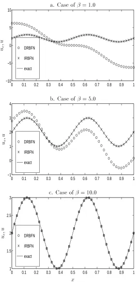
Consider the following 1D second order equation

r 2u =

;16

2sin(4 x) (25)

on 0 x 1 with u = 2 at x = 0 and x = 1. The exact solution can be veried to be

ue(x) = 2 + sin(4 x): (26)

This problem was solved by Dubal (1994) using the multiquadric approximation scheme in conjunction with a domain decomposition technique. Subdomains are built from 1D MQ approximation `template' which is an M M matrix

con-structed from multiquadric functions and their derivatives placed atM regularly spaced data points lying on the unit line. The best result with the \average per-centage relative error" of ;1:17e;2% was found in the case of 64 subdomains

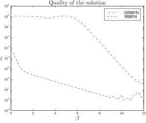
each of which contains 5 equally spaced points (M = 5) resulting in a total of 320 data points. In contrast, a total of 50 equally spaced points are used for the de-sign of both DRBFN and IRBFN procedures in the present work. The accuracy of the solution is more dependent on the value of in the case of DRBFN than in the case of IRBFN procedure as shown in Figures 2-3. Figure 3 shows that the IRBFN procedure achieves a better accuracy than the DRBFN procedure over a wide range of . However, at some large values of the DRBFN results are signicantly improved. For example, at = 8:0, the maximum errors are 2:08e;2% and 5:93e;6% for DRBFN and IRBFN respectively.

4.1.2 Example 2

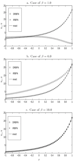
As a second example, consider the following equation

r 2u

;3ru + 2u = exp(4x) (27)

on ;1 x 1, which has the exact solution

(13)

Solving DEs using MQ RBFNs 13 and the boundary conditions are chosen so that B1 = 2 and B2 = 1. This

problem was also studied by Dubal (1994). Using the same method as mentioned in x4.1.1, Dubal reported that the minimum value of the \average percentage

relative error" was 9:23e;3% in the case of 32 subdomains with M = 5 (i.e.

160 data points). In the present methods, a total of 50 equally spaced points are used for the design of DRBFN and IRBFN. The observations on the DRBFN and IRBFN results (Figures 4 and 5) are similar to those indicated in the above example of x4.1.1. At = 8:0, the maximum errors are 1:98 % for DRBFN and

1:51e;5% for IRBFN.

4.2 Elliptic PDE in regularly shaped domain

In this section two examples in 2D are studied.

4.2.1 Example 1

The problem here is to determine a function u(x1x2) satisfying the following

PDE

r

2u = sin( x

1)sin( x2) (29)

on the rectangle 0 x1 1, 0 x2 1 subject to the Dirichlet conditionu = 0

along the whole boundary of the domain. The exact solution is given by ue(x1x2) =

;

1

2 2sin( x

1)sin( x2): (30)

This problem was solved using Feed Forward Neural Networks (FFNN) by Dis-sanayake and Phan-Thien (1994). The authors used the following congurations 2;3;3;1 (i.e. two input nodes followed by two hidden layers of three nodes

each and one output node), 2;5;5;1 and 2;10;10;1 to solve the problem

using the following data point densities 55, 1010 and 2020. The best results

obtained correspond to the last network architecture with the highest density. It is observed in the paper that the dierence in the accuracy of the solutions are not signicant between the last two congurations (i.e. 2;5;5;1 and 2;10;10;1)

and also between the two denser data distributions (i.e. 1010 and 2020).

The best FFNN results of Dissanayake and Phan-Thien (1994) are used here to compare with the present DRBFN and IRBFN solutions. The comparison ofNe

between FFNN, DRBFN and IRBFN solutions is shown in Figure 6 and it can be seen that the IRBFN solutions are the most accurate ones in all cases of data densities under consideration (i.e. 55, 1010 and 2020). The inuence of

(14)

Solving DEs using MQ RBFNs 14 7 which shows that increasing the data density makes theNe; curve more

sta-ble and results in an improvement of solution. However, the improvement only occurs at large values of for the DRBFN procedure in contrast with a wider range of values of for the IRBFN procedure. Furthermore, with in the range 5< < 8:6 the IRBFN solution has an norm of error of less than 10;6 in the case

of 2020 data density. Table 1 gives some indication of the rate of convergence

Table 1: Ne of FFNN and IRBFN solutions. The \improve factor" is dened

as ratio of Ne between two data densities. The FFNN results are taken from

Dissanayake and Phan-Thien (1994)

FFNN IRBFN( = 5:0) Density of 1010 1:40e;04 1:01e;05

Density of 2020 1:21e;04 5:72e;07

Improve Factor 1:15 17:65

of the solutions as the data density is increased for both the FFNN and IRBFN procedures. The table also shows that the IRBFN procedure appears to have a higher rate of convergence.

4.2.2 Example 2

In this example, the boundary conditions of the problem include both Dirichlet and Neumann type. Consider the following PDE

r

2u = (2 +2)exp(x

1+x2) (31)

on the rectangle 0 x1 1, 0 x2 1 with the following boundary conditions

u = exp(x1+x2) x2 = 0 and x2 = 1

u1 =exp(x1+x2) x1 = 0 and x1 = 1:

The exact solution is

ue(x1x2) = exp(x1 +x2): (32)

Here and are chosen to be 2 and 3 respectively. This problem was solved using the multiquadric approximation scheme by Kansa (1990b). The author used a total of 30 nodal points, including 12 scattered points in the interior and 18 along the boundary. The reported results showed that the norm of error is 1:66e;2

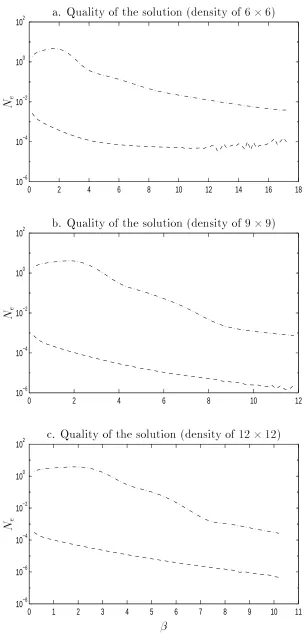
(this error gure is calculated by the present authors using the reported results of Kansa). In the present methods, the results obtained here are similar to those in the previous example. The IRBFN solution achieves greater accuracy in all cases (data density of 66, 99 and 1212) as shown in Figures 8 and 9. For

example, with the data density of 66 and = 8:0, the norms of error Nes are

(15)

4.3 Elliptic PDE in irregularly shaped domain

The 2D elliptic equation (17) subject to the boundary conditions (18)- (19) is reconsidered here. However, the domain in this case is irregularly shaped. Suppose that (17) is rewritten as

r

2u = p(

x) x2

(33)

which is subject to the same boundary conditions (18)-(19) as before. It can be seen that a solutionu(x) of (33), (18)-(19) is also a solution of the original system

(17)-(19). Based on this observation, a more convenient \superdomain" can

be chosen to replace the original domain subject to the condition

. The

boundary of the original domain therefore becomes an internal surface within .

For example, a convenient superdomain for the present 2D problem is a set of appropriate rectangles that is su"ciently large to completely cover the original domain with curved boundary (cf. Figure 10). A set of centres can then be regularly dened on this regular superdomain . The collocation points then

consist of all the centres and points used to dene the original boundary. For example, a set of uniformly distributed collocation points can be easily dened on and the boundary collocation points can be dened as the intersection

of the grid lines with the original boundary curve. Then, DRBFN and IRBFN are designed using the regularly shaped domain with only regularly distributed collocation points as RBF centres. The boundary conditions are decomposed into basis functions of the new domain of the network and imposed at the boundary points thus created.

For the purpose of illustration, let us consider the following Poisson's equation

r 2u =

;2 (34)

on an elliptical domain with semi-major axis of length a = 10 and semi-minor axis of length b = 8. The homogeneous condition u = 0 is imposed along the whole boundary. The exact solution is

ue(x1x2) = ;

a2b2

a2+b2

x2 1

a2 + x 2

2

b2 ;1

: (35)

The problem was solved using multiquadric approximation scheme by Sharan et al (1997). Due to the symmetry of this problem, the author considered only the rst quadrant of the ellipse using 28 data points. The maximum error was found to be 3:57e ;4% and the accuracy was up to ve signicant decimal places.

In the present methods, the rectangular superdomain used is 10 8 and the

density of centres is 119, which completely covers the elliptical domain (the

number of collocation points corresponding to the rst quadrant is the same as that of Sharan et al (1997)). The comparison of Ne between DRBFN and

(16)

Solving DEs using MQ RBFNs 16 is more accurate than the DRBFN one. The solutions corresponding to larger values of are very accurate. For example, at = 8:0, the accuracies are up to four signicant decimal places for DRBFN results and eight signicant decimal places for IRBFN results with maximum errors being 3:56e;3% and 2:27e;6%

respectively. To further demonstrate the accuracy of the methods the norm of error is calculated at 29 random points, which is 1:3561e;5 and 5:411e;7 for the

DRBFN and IRBFN procedures respectively. The maximum error is 1:58e;2%

and 3:80e;4% for the DRBFN and IRBFN procedures respectively.

4.4 Random collocation points

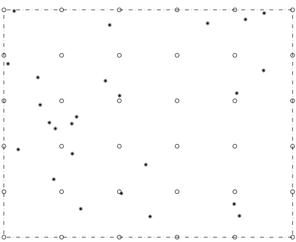
In the examples discussed so far the centres are also the collocation points in the case of regularly shaped domains. In the case of irregularly shaped domains, extra collocation points are generated on the curved boundary in order to accurately describe the boundary of the domain. In this section the eects of randomness of internal collocation points are investigated. Figure 1 illustrates the distribu-tion of regular RBF centres and random collocadistribu-tion points. The RBF centres are arranged on a regular grid and can be dierent from the collocation points. However, the set of collocation points can include the centres as a subset. The 2D example of x4.2.2 is reconsidered here with random collocation points. In order

to compare the present results with those of Kansa (1990b) the same number of internal random collocation points (12 points) and the same boundary colloca-tion points (18 points uniformly distributed) are used as shown in Figure 12. The centres (not shown) are uniformly distributed with a density of 66. Figure 13

shows that the present methods produce results which are more accurate than that reported by Kansa (1990b) for the same problem. Further improvements can be achieved by including the centres in the set of collocation points as shown in Figure 14. Note that this inclusion increases the number of collocation points without changing the number of unknowns. Figure 14 also shows that more ac-curate results are obtained by increasing the centre density as well as including the centres in the set of collocation points.

5 Discussion

5.1 Types of DEs and accuracy of the IRBFN method

(17)

Solving DEs using MQ RBFNs 17 are several orders of magnitude more accurate than those associated with the DRBFN method (accuracy is measured in terms of norm of error.) The above conclusion corresponds to the experimentally found \best" values of in the range of 7 to 10. Unfortunately, a theoretical determination of an optimal value for is, to our knowledge, not available. The better norm of error achieved in the IRBFN method is also underlined by a smooth error distribution over the entire domain as shown in Figures 15-17 where further comments can be found in the captions. Although the error distribution for the IRBFN is seen to be smooth in the present data-independent procedure (data-independent in the sense that the centres are xed and hence the kernel width is also xed according to 2 for a given ), Van Hulle (1998) showed that the kernel-based maximum entropy learning rule (kMER) can achieve equiprobabilistic topographic map formation for data-dependent nonparametric regression problems. The application of the latter method to the numerical solution of DEs will need further investigation in future work.

5.2 Why is the IRBFN method more accurate ?

A formal theoretical proof of the superior accuracy of the present IRBFN method cannot be oered at this stage, at least by the present authors. However, a heuristicargument can be presented as follows. In the direct methods, the starting point is the decomposition of the unknown functions into some nite basis and all derivatives are obtained as a consequence. Any inaccuracy in the assumed decomposition is usually magnied in the process of dierentiation. In contrast, in the indirect approach the starting point is the decomposition of the highest derivatives present in the relevant DEs into some nite basis. Lower derivatives and nally the function itself are obtained by integration which has the property of damping out or at least containing any inherent inaccuracy in the assumed shape of the derivatives.

5.3 RBFN and FFNN algorithms

(18)

Solving DEs using MQ RBFNs 18 determining the weights from some initial guess. Although back-propagation al-gorithm for the FFNN method is computationally e"cient, it suers from the problem of local minima (Haykin, 1999, pp229-232) and therefore convergence to the true solution is a very di"cult issue in the case of FFNNs (for example, the results of Dissanayake and Phan-Thien (1994) show that their FFNN method for the problem considered in x4.2.1 required 1000 iterations for convergence).

The results presented show that the system of algebraic equations becomes ill-conditioned at large , which is generally observed by other authors (Zerroukat et al, 1998). Too small values correspond to very localised approximation and when is too large the kernel becomes too at, loosing its ability to approxi-mate and therefore heuristically these two extremes would result in sub-optimal network performance as observed experimentally in this work. Even when the value of is in the \optimal" range, some peculiarities in the Ne- curve are

observed. Despite this peculiar behaviour, the IRBFN results are better than the corresponding DRBFN results. The reason for this peculiar behaviour is not clear. However, the results shown here indicate that the sudden drop in theNe

-curve (which represents a large improvement in accuracy) is due to a fortuitous combined eect of the centre density and the value of . As the centre density increases, this sudden drop disappears and the accuracy is better over the whole of the \optimal" range of for the IRBFN method (Figure 7b). The second pe-culiar behaviour is the oscillation observed at the tail of the Ne- curves, which

is also due to the combined eect of the centre density and the value. However, the reason here is probably due to the numerical ill-conditioning of the system matrix. This explanation is supported by the observation that the system matrix size for the IRBFN method is slightly more than twice the size of the DRBFN system matrix, leading to an earlier occurrence of the oscillatory behaviour as increases (Figure 6a). These peculiar behaviours can be eliminated with in-creasing centre density, however, at the expense of the freedom to choose in the sense that the range of optimal value is narrowed. Thus the present RBFN algorithms are stable for a range of value, provided that the centre density is su"cient, up to some critical value of above which the system matrix becomes nearly singular. A theoretical relationship for the balance between centre density and the value for requires formal investigation beyond the scope of the present work.

5.4 Other types of DEs

(19)

investiga-Solving DEs using MQ RBFNs 19 tion associated with the above discussion is beyond the scope of the present paper and will be carried out in the near future.

6 Concluding Remarks

New robust and highly accurate element-free procedures based on MQ RBFNs for solving DEs are discussed in this paper. The ease of preparation of input data (i.e. only discrete RBF centres and collocation points, which could be randomly or regularly distributed, are required), robustness of the methods (stability over a wide range of) and high accuracy of the solution (norm of error of O(1:0e;6)

at least for the IRBFN method with optimal value) make the method very attractive in comparison with conventional methods such as the FDM, FEM, FVM and BEM. Although the DRBFN method yields somewhat inferior norms of error of O(1:0e;3) (with optimal value), the mesh-free nature still makes

(20)

(21)

References

Brebbia, C.A., Telles, J.C.F., & Wrobel, L.C. (1984). Boundary Element

Tech-niques: Theory and Applications in Engineering. Berlin, Heidelberg:

Springer-Verlag.

Cook, R.D., Malkus, D.S., & Plesha M.E. (1989). Concepts and Applications of

Finite Element Analysis. Toronto: John Wiley & Sons.

Dissanayake, M. W. M. G. & Phan-Thien, N. (1994). Neural-Network-Based approximations for solving partial dierential equations. Communications

in Numerical Methods in Engineering, 10, 195-201.

Dongarra, J.J., Bunch, J.R., Moler, C.B. & Stewart G.W. (1979). LINPACK

User's Guide. Philadelphia: SIAM.

Dubal, M. R. (1994). Domain decomposition and local renement for multi-quadric approximations. I: Second-order equations in one-dimension.

Jour-nal of Applied Science and Computation, 1(1), 146-171.

Franke, R. (1982). Scattered data interpolation: tests of some methods.

Math-ematics of Computation, 38(157), 181-200.

Haykin, S. (1999). Neural Networks: A Comprehensive Foundation. New Jersey: Prentice-Hall.

Hughes, T.J.R. (1987) The nite element method, New Jersey:Prentice-Hall. Kansa, E. J. (1990a). Multiquadrics- A scattered data approximation scheme

with applications to computational uid-dynamics-I. Surface approxima-tions and partial derivative estimates. Computers and Mathematics with

Applications, 19(8/9), 127-145.

Kansa, E. J. (1990b). Multiquadrics- A scattered data approximation scheme with applications to computational uid-dynamics-II.Solutions to parabolic, hyperbolic and elliptic partial dierential equations. Computers and

Math-ematics with Applications, 19(8/9), 147-161.

Mai-Duy, N., & Tran-Cong, T. (1999). Approximation of function and its deriva-tives using radial basis function networks. Submitted to Neural Networks. Moody, J., & Darken, C.J. (1989). Fast Learning in Networks of Locally-tuned

Processing Units. Neural Computation, 1, 281-294.

(22)

Solving DEs using MQ RBFNs 22 Park, J. & Sandberg, I.W. (1993). Approximation and Radial Basis Function

Networks. Neural Computation, 5, 305-316.

Patankar, S.V. (1980)Numerical Heat Transfer and Fluid Flow, New York:McGraw-Hill.

Powell, M.J.D. (1988). Radial basis function approximations to polynomial. In D.F. Gri"ths & G.A. Watson (Eds), Numerical Analysis 1987 Proceedings

(pp. 223-241), Dundee, UK: University of Dundee.

Press, W.H., Flannery, B.P., Teukolsky, S.A., & Vetterling, W.T. (1988).

Nu-merical Recipes in C: The Art of Scientic Computing. Cambridge:

Cam-bridge University Press.

Sharan, M., Kansa, E. J. & Gupta, S. (1997). Application of the multiquadric method for numericalsolution of elliptic partial dierential equations.

Jour-nal of Applied Science and Computation, 84, 275-302.

Smith, G.D. (1978)Numerical Solution of Partial Dierential Equations: Finite

Dierence Methods, Oxford:Claredon Press.

Tarwater, A. E. (1985). A parameter study of Hardy's multiquadric method for scattered data interpolation. Technical Report UCRL-563670. Lawrence Livemore National Laboratory.

Van Hulle, M. M. (1998). Kernel-Based Equiprobabilistic Topographic Map Formation. Neural Computation, 10, 1847-1871.

Zerroukat, M., Power, H. & Chen, C.S. (1998). A numerical method for heat transfer problems using collocation and radial basis functions. International

Journal For Numerical Methods in Engineering, 42, 1263-1278.

(23)

Figure 1: RBF centres and collocation points. Legends : RBF centre and :

[image:23.612.133.431.143.387.2]

(24)

DRBFN IRBFN exact

0 0.1 0.2 0.3 0.4 0.5 0.6 0.7 0.8 0.9 1 −10

−5 0 5 10

DRBFN IRBFN exact

0 0.1 0.2 0.3 0.4 0.5 0.6 0.7 0.8 0.9 1 −1

0 1 2 3 4

DRBFN IRBFN exact

0 0.1 0.2 0.3 0.4 0.5 0.6 0.7 0.8 0.9 1 1

1.5 2 2.5 3

x

ue

u

ue

u

ue

u

a. Case of = 1:0

b. Case of = 5:0

c. Case of = 10:0

Figure 2: Solution of r 2u =

;16

2sin( x): plots of the exact solution and the

[image:24.612.152.435.32.613.2]

(25)

0 1 2 3 4 5 6 7 8 9 10 11 12 13

10−10 10−8 10−6 10−4 10−2 100 102

DRBFN IRBFN

Ne

Quality of the solution

Figure 3: Solution of r 2u =

;16

2sin( x): comparison of N

e between DRBFN

[image:25.612.136.431.144.390.2]

(26)

DRBFN

IRBFN

exact

DRBFN

IRBFN

exact

DRBFN

IRBFN

exact

−1 −0.8 −0.6 −0.4 −0.2 0 0.2 0.4 0.6 0.8 1

−5 0 5 10 15 20 25

−10 −0.8 −0.6 −0.4 −0.2 0 0.2 0.4 0.6 0.8 1

5 10 15 20 25

−10 −0.8 −0.6 −0.4 −0.2 0 0.2 0.4 0.6 0.8 1

5 10 15 20 25

x

ue

u

ue

u

ue

u

a. Case of = 1:0

b. Case of = 6:0

c. Case of = 10:0

Figure 4: Solution of r 2u

;3ru + 2u = exp(4x): plots of the exact solution

[image:26.612.154.432.32.657.2]

(27)

0 2 4 6 8 10 12

10−9 10−8 10−7 10−6 10−5 10−4 10−3 10−2 10−1 100 101

DRBFN IRBFN

Ne

Figure 5: Solution of r 2u

;3ru + 2u = exp(4x): comparison of Ne between

[image:27.612.134.431.147.398.2]

(28)

0 5 10 15 20 25

10−6 10−4 10−2 100 102

0 1 2 3 4 5 6 7 8 9 10 11

10−8 10−6 10−4 10−2 100 102

0 1 2 3 4 5 6 7 8 9

10−8 10−6 10−4 10−2 100 102

Ne

a. Quality of the solution (density of 55)

b. Quality of the solution (density of 1010)

c. Quality of the solution (density of 2020)

Figure 6: Solution ofr

2u = sin( x

1)sin( x2): comparison ofNe between FFNN,

DRBFN and IRBFN procedures with some centre densities: 55, 1010 and

20 20. Solid line: FFNN, dashdot line: DRBFN and dashed line: IRBFN.

[image:28.612.127.430.21.663.2]

(29)

0 1 2 3 4 5 6 7 8 9

10−4 10−3 10−2 10−1 100 101

0 1 2 3 4 5 6 7 8 9

10−8 10−7 10−6 10−5 10−4 10−3 10−2 10−1

Ne

a. Case of DRBFN

b. Case of IRBFN

Figure 7: Solution of r

2u = sin( x

1)sin( x2): eect of centre density on Ne of

DRBFN and IRBFN results. Dashdot line: density of 55, dashed line: density

of 1010 and solid line: density of 2020. In this plot the behaviours of the

[image:29.612.131.435.138.603.2]

(30)

0 2 4 6 8 10 12 14 16 18

10−6 10−4 10−2 100 102

0 2 4 6 8 10 12

10−6 10−4 10−2 100 102

0 1 2 3 4 5 6 7 8 9 10 11

10−8 10−6 10−4 10−2 100 102

Ne

a. Quality of the solution (density of 66)

b. Quality of the solution (density of 99)

c. Quality of the solution (density of 1212)

2u = (2+2)exp(x

1+x2): comparison of Ne between

DRBFN and IRBFN procedures with data densities: 66, 99, 1212. Dashdot

[image:30.612.128.432.58.694.2]

(31)

1 2 3 4 5 6 7 8 9 10 11

10−4

10−2

100

102

1 2 3 4 5 6 7 8 9 10 11

10−6

10−4

10−2

Ne

a. Case of DRBFN

b. Case of IRBFN

2u = (2 +2)exp(x

1+x2): eect of data density on

Ne of DRBFN and IRBFN results. Dashdot line: density of 66, dashed line:

density of 99 and solid line: density of 12 12. In this plot the behaviours

[image:31.612.132.432.149.597.2]

(32)

Figure 10: Regularly extended domain: In the present work, a regularly shaped domain is dened as a rectangular region in 2D or a parallelepiped region in 3D. For example, a 2D regular domain is dened by a x1 b c x2 d where

[image:32.612.132.432.58.302.2]

(33)

0 1 2 3 4 5 6 7 8 9

10−9 10−8 10−7 10−6 10−5 10−4 10−3 10−2 10−1 100

DRBFN IRBFN

Ne

Figure 11: Poisson's equation in an elliptical domain: comparison of Ne between

DRBFN and IRBFN procedures.

0 0.2 0.4 0.6 0.8 1

0 0.25 0.5 0.75 1

x1

x2

Figure 12: Random internal collocation points for the solution of r 2u =

(2 + 2)exp(x

1 +x2). Legends

: internal random point and :

[image:33.612.130.430.36.283.2] [image:33.612.134.431.356.591.2]

(34)

0 5 10 15

10−4 10−3 10−2 10−1 100 101

Kansa (1990) DRBFN IRBFN

Ne

Quality of the solution (density of 66)

2u = (2+2)exp(x

1+x2): Comparison ofNebetween

[image:34.612.133.430.179.438.2]

(35)

0 1 2 3 4 5 6 7 8 9 10

10−5 10−4 10−3 10−2 10−1

Density of 6*6 Density of 6*6 Density of 7*7 Density of 8*8

Ne

Quality of the solution (12 random points)

Figure 14: Solution of r

2u = (2+2)exp(x

1 +x2): Eect of centre density

on Ne of IRBFN solution. The top curve corresponds to the case where the

[image:35.612.134.428.181.428.2]

(36)

0 0.25

0.5 0.75

1

0 0.25 0.5 0.75 1 −6.5 −6 −5.5 −5 −4.5 −4

0 0.25

0.5 0.75

1

0 0.25 0.5 0.75 1 −14 −12 −10 −8

x1

x2

log

(absol

ute

err

or)

log

(absol

ute

err

or)

a. Case of DRBFN

b. Case of IRBFN

Figure 15: Error in the solution of r

2u = sin( x

1)sin( x2): the numerical

[image:36.612.130.433.78.538.2]

(37)

0 0.25

0.5 0.75

1

0 0.25 0.5 0.75 1 −3.5 −2.5 −1.5 −0.5 0.5

0 0.25

0.5 0.75

1

0 0.25 0.5 0.75 1 −7 −6 −5 −4 −3

x1

x2

log

(%

rela

tiv

e

erro

r)

log

(%

rela

tiv

e

erro

r)

a. Case of DRBFN

b. Case of IRBFN

Figure 16: Error in the solution ofr

2u = (2+2)exp(x

1+x2): the numerical

[image:37.612.131.435.85.543.2]

(38)

−10 −5

0 5

10

−10 −5 0 5 10 −6 −4 −2

−10 −5

0 5

10

−10 −5 0 5 10 −15 −10 −5

x1

x2

log

(%

rel

ativ

e

err

or

)

log

(%

rel

ativ

e

err

or

)

a. Case of DRBFN

b. Case of IRBFN

Figure 17: Error in the solution of r 2u =

;2: the numerical solutions are

[image:38.612.134.433.71.531.2]