A novel method for detecting outlying subspaces in high-dimensional databases using genetic algorithm

A Novel Method for Detecting Outlying Subspaces in High-dim ensional

Databases Using Genetic Algorithm

Ji Zhang, Qigang Gao

Faculty of Computer Science

Dalhousie University

Halifax, Nova Scotia, Canada

{

jiz, qggao

}

@cs.dal.ca

Hai Wang

Sobey School of Business

Saint Mary’s University

Halifax, Nova Scotia, Canada

[email protected]

Abstract

Detecting outlying subspaces is a relatively new research problem in outlier-ness analysis for high-dimensional data. An outlying subspace for a given data pointpis the sub-space in whichpis an outlier. Outlying subspace detection can facilitate a better characterization process for the de-tected outliers. It can also enable outlier mining for high-dimensional data to be performed more accurately and effi-ciently. In this paper, we proposed a new method using ge-netic algorithm paradigm for searching outlying subspaces efficiently. We developed a technique for efficiently comput-ing the lower and upper bounds of the distance between a given point and itskth _{nearest neighbor in each possible}

subspace. These bounds are used to speed up the fitness evaluation of the designed genetic algorithm for outlying subspace detection. We also proposed a random sampling technique to further reduce the computation of the genetic algorithm. The optimal number of sampling data is speci-fied to ensure the accuracy of the result. We show that the proposed method is efficient and effective in handling out-lying subspace detection problem by a set of experiments conducted on both synthetic and real-life datasets.

1

Introduction

Outlier detection is an important research problem in data mining that aims to find a specific number of ob-jects that are considerably dissimilar, exceptional and consistent with respect to the majority records in the in-put databases. Numerous research work in outlier detection has been proposed such as the distribution-based methods [3][6], the distance-based methods [9][10][12], the density-based methods [2][8][13] and the clustering-density-based methods [1][5][7][11][15][19], etc.

In this paper, we focus on the problem ofoutlying

sub-space detectionfor high dimensional data, which is a com-plementary problem of outlier detection. The major task of outlying subspace detection is to find the subspaces (subsets of features) in which each data point exhibits significant de-viation from the rest of population. An outlying subspace for a data point is a subspace (a subset of features) in which this data can be considered as an outlier. The problem of outlying subspace can be formulated as follows: given a data point, find the subspaces in which this point is consid-erably dissimilar, exceptional or inconsistent with respect to the remaining population in the database[14].

outly-ing subspace detection can help outlier detection methods to mine outliers in high-dimensional space more efficiently. It is an important intermediate step inexample-based out-lier mining, which detects outout-liers based on a set of outout-lier examples supplied by domain experts [16][17]. The basic idea of this method is to find the outlying subspaces of these outlier examples, from which more outliers that have sim-ilar outlier-ness characteristics to the given examples can be found more efficiently by only investigating the detected outlying subspaces.

Unfortunately, due to the exponential growth of the number of subspaces with respect to the dimension of the dataset, the problem of outlying subspace detection is NP-hard by nature. The straightforward exhaustive search is apparently infeasible to this problem, especially for high-dimensional datasets. In response to the inherent hardness of this problem, the state-of-the-art methods were proposed to employ heuristics in speeding up the search process in order to render this problem tractable. Zhang et al. pro-posed a dynamic outlying subspace search algorithm that utilizes a sample-based learning process to efficiently iden-tify the outlying subspaces for the given points [14][18]. Two heuristic pruning strategies employing the upward and downward closure property are devised to reduce search space. Its major drawbacks, however, lie in the unsatisfac-tory accuracy of the metric used for measuring outlying de-gree of points in subspaces, the binary fashion of its result and the difficulty in specifying the distance threshold. Zhu et al. draw on a genetic algorithm to solve the example-based outlier detection problem [16][17]. The major limita-tion of this method is that it is computalimita-tionally expensive to compute the outlying degree of points in subspaces. This is because that it uses a cell-based partitioning technique that scales poorly in high-dimensional space.

In this paper, we develop a method based on genetic al-gorithm to solve the outlying subspace detection problem that well copes with the drawbacks of the existing methods. The main contributions of this paper are summarized as fol-lows:

1. A new metric, calledSubspace Outlying Factor(SOF), is developed for measuring the outlying degree of each data point in different subspaces. Based on SOF, a new definition of outlying subspace, called SOF Outlying Subspaces, is proposed. The parameters used in defin-ing SOF Outlydefin-ing Subspaces are easy to be specified, and do not require any prior knowledge about the data distribution of the dataset;

2. A genetic algorithm-based method is proposed for out-lying subspace detection. The upward and downward closure property is no longer required in our GA-based method, and the detected outlying subspaces can be ranked based on their fitness function values;

3. The concepts of the lower and upper bounds of Dk, the distance between a given point and itskthnearest neighbor, are proposed. These bounds are used for a significant performance boost in our method. We pro-pose a technique to compute these bounds efficiently using the so-calledkNN Look-up Table;

4. The random sampling technique is utilized in our method to further speed up the computation. The opti-mal number of sampling data is specified, and a novel genetic algorithm is developed to combine incremental data sampling and subspace fitness evaluation;

5. Last but not the least, we show that the proposed method is efficient and effective in handling outlying subspace detection problem through experiments con-ducted on both synthetic and real-life datasets.

2

Problem Formulation

To define outlying subspace, we need to first devise the metric for measuring outlier-ness of the given data point in different subspaces. In this work, we useDk_{, the distance}

between a point and itskthnearest neighbor, in our outlier-ness metric, calledSubspace Outlying Factor (SOF). Math-ematically, the SOF of a subspacesw.r.t a given pointpis defined as the ratio ofDk_{(p)insagainst the averagedD}k

insfor points in the datasetD, i.e.

SOF(s, p) = D k s(p)

Dk s(D)

(1)

Intuitively, the higher the ratio is, the higher theDk _ofpis

when compared to other points, therefore the higher outlier-ness ofpis and vice versa. Our definition of SOF leads to the following definition ofSOF Outlying Subspaces:

Definition 1. SOF Outlying Subspaces: Given an

in-put datasetD, parametersnandk, a subspacesis aSOF Outlying Subspacefor a given data pointpif there are no more thann−1other subspacess′such thatSOF(s′_{, p)>}

SOF(s, p).

The above definition is equivalent to say that the topn

subspaces having the largest SOF values are considered to be outlying subspaces.

3

Lower and Upper Bounds of

D

As the lower and upper bounds ofDkof data points are established by means of their respectivekNN Lookup Ta-ble, we therefore first introducekNN Lookup Table prior to our discussion on the bounds ofDk_.

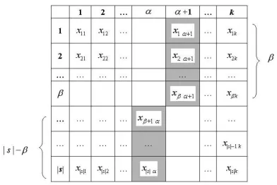
Definition 2: Full kNN Lookup Table: A Full kNN

Figure 1. PartialkNN Lookup Table of a data point

containing information about itsknearest neighbors ineach single dimension of full data space withϕdimensions. The entryxij of the table represents thejthnearest neighbor of

pin theith_{dimension, where1≤i≤ϕand1≤j≤k.}

It is important to note that the lower and upper bounds of

Dk_{(p)will vary in different subspaces and only a portion of}

Tp _{is actually used to construct the bounds ofD}k_{(p)in a}

particular subspaces. That is, only the dimensions relevant tosare needed to be considered. As such, we propose the notion of PartialkNN Lookup Table that is defined as a view of the corresponding fullkNN Lookup Table.

Definition 3: PartialkNN Lookup Table:A PartialkNN

Lookup Table of a datapwith respect to a subspaces, de-noted as Tp

s, is a|s| ×k view (logical table) of the full

kNN Lookup Table ofp, with each entryxij being thejth

nearest neighbor ofpin theith_{dimension, whered}

i ∈ s,

1 ≤i ≤ |s|and1 ≤ j ≤ k. |s|is the number of dimen-sions ofs. Apparently, the PartialkNN Lookup Table is a selection of its corresponding fullkNN Lookup Table, i.e.

Tp

s =σdi∈sTp.

3.1

Lower Bound of

Given a subspacesand the number of nearest neighbor

k, we will first calculate the following two constructs,αand

β. These two constructs will be utilized in constructing the lower bound ofDk_{ofpins.αandβare defined as follows:}

(

α=jk−1

|s|

k

+ 1

β= (k−1)mod|s| (2)

wherejk_|−1_s| kdenotes the maximum integer that does not

exceedk_|−1_s| .

Whenαandβ are available, we sortTp

s based on the

values ofDα

di(p), the distance betweenpand itsα

th_nearest

neighbor in di (di ∈ s) and select the β dimensions that

have the lowest Dαdi(p) values which are presented in set

d′:

d′={d1, d2, . . . , dβ} (3)

Then we define theLower Bound Set(LBS)ofpinsas

LBSs(p) ={e1, e2, . . . , e|s|} (4)

where each elementei (1 ≤ i ≤ |s|) is a positive integer

and specified as follows:

ei=

α+ 1,ifdi∈d′

α, ifdi6∈d′

(5)

The lower bound ofDk_{(p)for a pointpins, denoted as}

LBs(Dk(p)), is given as

LBs(Dk(p)) =

s P|s|

i=1D

ei

di(p)

2

|s| −1 , ei∈LBSs(p) (6)

whereDei

di(p)denotes the distance between pand itse

th i

nearest neighbor in dimensiondi ∈s.

Figure 1 presents the Partial kNN Lookup Table of a point. All the elements inLBSs(p)has been highlighted

using darker background in the table. As we discussed ear-lier, there are|s|elements inLBSs(p); the first|s| −β

ele-ments come from Columnαand anotherβ elements come from Columnα+ 1. These|s|elements inLBSs(Dk(p))

form alower bound frontierin the PartialkNN Lookup Ta-ble.

Lemma 1:

r

P|s|

i=1D ei di(p)

2

|s|−1 , ei ∈ LBSs(p) is the lower

bound ofDk_{(p)for a pointpin subspaces.}

Proof: LetN N Index(p,di)(q)be nearest neighbor index

number of pointqwith respect topin dimensiondiof

sub-spaces. For instance, ifqis the10th_{nearest neighbor ofp}

in the5th_{dimension of}

s, thenN N Index(p,d5)(q) = 10. The total number of unique points q such that

N N Index(p,di)(q) < ei for any dimensiondi ins,1 ≤

i≤ |s|(i.e. falling to the left side of the lower bound fron-tier of the table) is no more thank−1. Without losing gen-erality, let us suppose that there aret such unique points, (1≤t≤k−1).

For any pointqsatisfyingN N Index(p,di)(q) ≥ eifor

all the dimensions di of s, 1 ≤ i ≤ |s| (i.e. locating

to the right of the lower bound frontier of the table), we havedistdi(p, q) ≥ D

ei

di(p)for eachdi ∈ s. Therefore,

dists(p, q)≥

r

P|s|

i=1D ei di(p)

2

|s|−1 .

Suppose, among thetunique points locating to the left of the lower bound frontier of the table, there aret′ _points

q satisfyingN N Index(p,s)(q) ≤ t (0 ≤ t′ ≤ t). Then, the (t′ _{+ 1)}th _{nearest neighbor of p in s should locate}

to the right of the lower bound frontier and Dt′+1

s (p) ≥

r

P|s|

i=1D ei di(p)

2

t′+ 1 ≤ k andDst′+1(p) ≤ D k

s(p). Given D

t′₊₁

s (p) ≥

r

P|s| i=1D

ei di(p)

2

|s|−1 and D

t′+1

s (p) ≤ Dks(p), then we have

Dk

s(p)≥

r

P|s| i=1D

ei di(p)

2

|s|−1 , as required.

3.2

Upper Bound of

To compute the upper bound ofDk_{(p)ofpins, we need}

to first obtain theUpper Bound Set(UBS) forpins. It is defined as follows:

U BSs(p) =∪|is=1| KN N Setdi(p), di∈s (7)

whereKN N Setdi(p)denotes the set ofkNNs ofpin

di-mensiondi and it represents each row ofTsp. Obviously,

we havek≤ |U BSs(p)| ≤k|s|.|U BSs(p)|=kwhen the

kNNs ofpin each dimensiondi∈sare identical, whereas

|U BSs(p)| =k|s|when there are no duplicates inTsp. In

computing the lower bound ofDk_{(p),U BS}

s(p)is used to

store the result of union operation on allkNN sets ofpin each single dimension.

Let pointqbe thekth_{nearest neighbor ofpinU BS}

s(p).

The upper bound ofDk _{ofpinsis defined as the distance}

betweenpandqinsas

U Bs(Dk(p)) =dists(p, q) (8)

Lemma 2. Let pointqbe thekth_{nearest neighbor ofpin}

U BSs(p), thendists(p, q)is the upper bound ofDkofpin

s.

Proof: For two setsset1 andset2such thatset1 ⊆ set2

and|set2| ≥ |set1| ≥ k, if q1 and q2 are the kth near-est neighbor ofp inset1 andset2, respectively, then we havedists(p, q1)≥ dists(p, q2). This is because thatDk is monotonically decreasing as the set of points we examine gets larger.

Now let set1 and set2 be instantiated as set1 =

U BSs(p) and set2 = D, where D denotes the whole dataset, we thus have U BSs(p) ⊆ D and |D| ≥

|U BSs(p)| ≥ k. Based on the above discussion, we will

havedists(p, q1) ≥ dists(p, q2), whereq1 andq2 are the

kth_{nearest neighbor ofpinU BS}

s(p)andD, respectively.

Therefore,dists(p, q1)is the upper bound ofDk ofpins, as desired.

3.3

Approximation of Subspace Outlying Factor

by Using Bounds of

LetLBs(Dk,D)andU Bs(Dk,D)be the average lower

and upper bounds ofDkin subspacesfor points in dataset

D. We define the minimum and maximum values for SOF ofpinsas follows:

SOFmin(s, p) =

LBs(Dk(p))

U Bs(Dk,D)

SOFmax(s, p) =

U Bs(Dk(p))

LBs(Dk,D)

(9)

The approximated SOF of s with respect to p is computed by using the average of SOFmin(s, p) and

SOFmax(s, p)as follows:

SOFapp(s, p) =

SOFmin(s, p) +SOFmax(s, p)

2 (10)

3.4

Performance Improvement Using

Approxi-mation of SOF

As pointed out in [13], kNN search in subspace sfor all the N points in the database requires a complexity of

O(k|s|N2_{)whensis of a high dimension.}

If our approximation scheme of SOF is used, comput-ing the lower bound of Dk_{(p) in s only requires}

sort-ing the αth _{column of T}p

s and summing up D ei

di(p)

2 _for

each di ∈ s, with a complexity of O(|s|log|s| + |s|).

While for computing the upper bound of Dk_{(p)in s, we}

need to find the kth_{NN of p in U BS}

s(p) with a

maxi-mum possible size ofk|s|. Hence, the complexity will be

O(k|s| ·k|s|) =O(k2_|s|2_{). In sum, the complexity of} com-puting the bounds ofDk_{for all the points in the database is}

O((|s|log|s|+|s|+k2|s|2_{)N) =O(k}2_|s|2_N).

By using our approximation technique, we are able to reduce the complexity in computing SOF of a subspace to a linear order with respect toN, leading to a computation saving by up to a factor of _kN_|s| compared to the case when no approximation is performed. SinceN >> |s|andkis usually small in most cases, our approximation technique is thus able to achieve a significant performance improvement.

4

Construction of

k

NN Look-up Table

ThekNN Look-up Table for a data point should be first constructed before its lower and upper bounds ofDk _can

thereby be established. The key task involved in construct-ing the kNN Look-up Table of a data point is to find its

kNNs in each single dimension of the full data space. To facilitate construction of the tables, we transform the orig-inal dataset into a few sorting lists, where the number of the sorting lists is equal to the number of dimensions of the dataset. Each sorting list is constructed based on the sorting order of data in each dimension. The lengths of all sort-ing lists are identical and equal to the number of data points in the original dataset. Each element in the sorting list has two fields: the ID and the value of a particular point in the related dimension. There can be a few ways to implement

kNN search in the sorting lists. In this work, we will study three simple yet efficient methods, namely the list-based, block-based and tree-based methods.

List-based Method.kNN search can be performed directly

subsequentk points of pare the candidates of its kNNs, from whichkNNs ofpcan be found.

Locating a pointpin any one sorting list needs a com-plexity of O(log2N)and findingkNNs in the sorting list requires another O(k)computation. In sum, the compu-tational complexity of employing the sorting list will be

O(log2N+k). The space complexity of list-based method isO(2N).

Lemma 3: If a sorting list is partitioned into blocks with

an equal sizeb, then at most 3 blocks in the sorting list are needed to be searched for findingkNNs for any pointpif

b ≥ k. These 3 blocks are the blockBto whichpbelong and the the two adjacent blocks ofB.

Proof: Without losing generality, let us suppose that the

sorting list is related to dimensiondi(1 ≤i ≤ϕ) and the

block index number ofB to whichpbelongs isi. For any pointqin Block(i−2), there are at leastkpoints in Block

i−1whose distance topin dimensiondiis less than or equal

todistdi(p, q). Likewise, for any pointqin Block(i+ 2),

there are at leastkpoints in Block(i+ 1)whose distance topin dimensiondi is less than or equal to distdi(p, q).

Therefore, allkNNs ofpdefinitely fall into Block(i−1),i

or(i+ 1).

Block-based Method . kNN search can also be performed

on a block-by-block basis. The basic idea is to partition a sorting list into a number of blocks. These blocks are usually of an equal size and contain more than k points. Each time, only a single block is evaluated. LetBminand

Bmaxbe the minimum and maximum point values in the

current block being loaded, respectively, andp.valuebe the value ofpin the sorting list. IfBmin ≤p.value≤Bmax,

then this block is the one to whichpbelongs. We can further locate pin this block and performkNN search for p. If

Bmin≤p.value≤Bmaxis not met for the current block,

then another block will be loaded for evaluation.

The computational complexity for finding the block to whichpbelongs isO(1)for the best case wherepis located in the first block we evaluate andO(N

b)for the worst case

where all the blocks in the sorting list are exhausted in the search. The average-case complexity is thusO(N+b

2b ). Also,

the time complexity for locatingpin the block isO(log2b). FindingkNNs in the sorting list requires anotherO(k) com-putation. The total time complexity isO(N+b

2b +log2b+k).

Since at most 3 blocks in the sorting list need to be searched, the space complexity is thereforeO(6b).

Tree-based Method. The third alternative is to utilize a

tree structure to further index the data blocks in the sorting list. For the sake of simplicity, we constructBinary Trees for performance enhancement inkNN search. Binary tree is simple in structure yet very efficient inkNN search.

The binary tree we use for each sorting list is a balanced rooted treeBT =< V, E >, whereV is the node set and

E is the edge set. The nodes in V are classified as the

block nodesand theindexing nodes. Theblock nodesare the leaves of the binary tree that represent data blocks in a sorting list that each containsbpoints, whereb≥k. Each data block in the leaf level will be represented by its mini-mum point value (the first value in the block if the sorting list is ordered in an ascending order) in the binary tree. The indexing nodesare other nodes in the tree primarily used for indexing the data blocks at the bottom level. The immedi-ate indexing node of a block node takes the smallest value and the starting address of the data block. Other indexing nodes (excluding the root) will take the minimum value of its children, together with the addresses of its left and right children. The root will only stores the addresses of its two children.

kNN search for a pointpin a binary tree also takes two major steps. First, the binary tree is traversed top-down from the root until the block to which pbelongs is found. The moment an intermediate indexing node ais reached, the following rule is used to decide the sub-tree for further traversal: Ifp.value≥ a.rightchild, then right child ofa is chosen for traversal. Otherwise, the left child is selected for traversal. When a bottom indexing node (i.e. the im-mediate parent of a block node) is reached, the block node to which it is pointing is referred and the whole data block is fetched. After the block to whichpbelongs to has been found, the location ofpwithin the block will be determined andkNN search can be performed.

It will require O(log2Nb) to traverse the binary tree

downward from the root to find the block to which p be-longs. The complexity of locatingpin the block isO(log2b) and searching for kNNs ofpin 3 blocks requires a com-plexity ofO(k). In sum, the time complexity isO(log2N_b +

log2b+k) =O(log2N+k).

The total number ofindexing nodesin the tree is approx-imately 2_bN. We load all the indexing nodes of the binary tree as they will be frequently used forkNN search. Since it is not required to load any data blocks until the block to whichpbelong has been found and at most 3 blocks are needed to be loaded forkNN search for p, thus the space complexity of tree-based method isO(2N

b + 6b).

5

Genetic Algorithm for Detecting Outlying

Subspaces

In this section, we will elaborate on the design of the genetic algorithm for outlying subspace detection.

Representation. Our GA technique uses the standard

bi-nary individual encoding; all individuals are represented by strings with fixed and equal lengthϕ, whereϕis the num-ber of dimensions of the dataset. Using binary alphabet

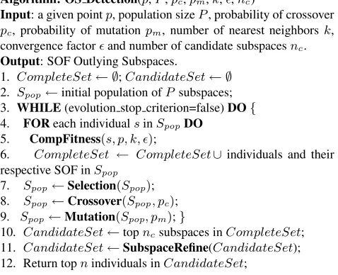
Algorithm: OS Detection(p,P,pc,pm,k,ǫ,nc)

Input: a given pointp, population sizeP, probability of crossover pc, probability of mutationpm, number of nearest neighborsk,

convergence factorǫand number of candidate subspacesnc.

Output: SOF Outlying Subspaces.

1. CompleteSet← ∅;CandidateSet← ∅

2. Spop←initial population ofPsubspaces;

3. WHILE(evolution stop criterion=false)DO{

4. FOReach individualsinSpopDO

5. CompFitness(s, p, k, ǫ);

6. CompleteSet ← CompleteSet∪ individuals and their respective SOF inSpop

7. Spop←Selection(Spop);

8. Spop←Crossover(Spop, pc);

9. Spop←Mutation(Spop, pm);}

10. CandidateSet←topncsubspaces inCompleteSet;

11. CandidateSet←SubspaceRefine(CandidateSet); 12. Return topnindividuals inCandidateSet;

Figure 2. Genetic algorithm for outlying sub-space detection

Fitness Function. The fitness function used in the genetic

algorithm is defined as the approximated SOF of subspace

swith respect to the given pointp, as presented in Eq. (10), i.e.

ff it(s) =SOFapp(s, p) =

SOFmin(s, p) +SOFmax(s, p) 2

(11)

A higher value offf it(s)indicates a fitter solution and vice

versa. The definition offf it(s)encourages the genetic

algo-rithm to produce an increasing number of subspaces having high SOF values as evolution proceeds.

Selection Operator.In our work,fitness-proportionate

se-lection, also known as roulette-wheel selection, is used to select fitter solutions in each step of the evolution. Fitness-proportionate selection is a stochastic selection method where the selection probability of a subspace is proportional to the value of its fitness functionff it(s).

Search Operators.The crossover and mutation used in this

work issingle-point crossoverandbit-wise mutation. In our work, all the new individuals generated by crossover and mutation are of the same length, i.e. ϕ, as their parent(s), where ϕ is number of dimensions of the input database. There are two associated probabilities,pc andpm, used to

determine the frequencies for applying crossover and muta-tion, respectively. Normally, we havepc >> pm, meaning

that crossover is performed in a much higher frequency than mutation.

Algorithm. The framework of genetic algorithm for

detecting outlying subspace is presented in Figure 2.

CompleteSetis the set used to maintain all the subspaces,

together with their respective SOF, that have been evalu-ated in the genetic algorithm andCandidateSetis the set used to only store the candidates of SOF Outlying Sub-spaces. The stopping criterion in the WHILE loop is usu-ally that the number of generations performed has reached a pre-specified constant. CandidateSetstores the topnc

subspaces inCompleteSet (line 10). In order to achiev-ing good accuracy of the detected outlyachiev-ing subspaces, nc

should be substantially larger than n. In Line 11, we perform subspace refinement (will be discussed in the se-quel) and the top nsubspaces from all the candidates in

CandidateSetare returned as SOF Outlying Subspaces.

The Subspace Refinement. Since we approximate SOF in

the genetic algorithm, the accuracy of computation is thus somehow limited. To address this problem, we can perform a refinement step on the candidate outlying subspaces in Line 11 of the genetic algorithm (Figure 2). Instead of us-ing the lower and upper bounds ofDk _{for a fast fitness}

ap-proximation, the refinement step will compute the accurate SOF for all subspace candidates inCandidateSetand the topnoutlying subspaces among them will be returned. A pruning optimization strategy can be devised based on the maximum value of SOF (i.e. SOFmax) of different

sub-spaces to speed up the computation. The basic idea of this pruning optimization strategy is that, afternsubspace can-didates have been evaluated, we start to maintain the mini-mum value of SOF for the topnsubspaces we have found thus far, denoted asM inSOFn. Those subspaces satisfying

SOFmax(s, p)< M inSOFncannot become the topn

sub-spaces and can therefore be safely pruned. This is because that the value ofM inSOFnis monotonically increasing as

more subspaces are examined in the refinement step.

6

Random Sampling

The most computationally expensive step in our genetic algorithm lies in the fitness evaluation of individuals. This is because that the fitness evaluation for each subspace, either in approximated or accurate manner, involves scanning all the points in the dataset. This will be slow as the number of points in the dataset is usually large. To speed up fitness evaluation, we draw on random sampling technique so as to evaluate fitness of individuals only based on the random samples, rather than on the entire dataset.

By using sampling data, the average lower and upper bounds ofDk _{in subspaces, used in SOF approximation,}

can be computed as follows:

LBs(Dk,S) =

1 NS

NS

X

i=1

LBs(Dk(spi))

U Bs(Dk,S) =

1 NS

NS

X

i=1

whereNSdenotes the number of points in the sampleSand

spidenotes theithsampling point inS,1≤i≤NS. Sampling can help improve the efficiency of our method significantly, but the quality of the result may be affected. In what follows, we will discuss convergence of the aver-aged lower and upper bounds of Dk _{when the number of}

sampling data is increased.

LetXbe a variable that can represent the averaged lower or upper bound ofDk_{for a set of data points in a subspace.}

Let us suppose that there are alreadyi−1sampling points and theith_{sampling point is generated. From the}

conver-gence perspective, we want to ensure that∃µ≥2, whereµ

is a positive integer, for∀i≥µ, we have

|Xi−Xi−1|

Xi−1

< ǫ (13)

whereXi denotes the average value ofX for all the first

i sampling points. ǫ is called convergence factor and is usually a small positive number (say 0.01). The ratio of

|Xi−Xi−1|

Xi−1 < ǫmeasures the degree to which the averaged value ofXchanges due to the inclusion of the new (i.e. the

ith) sample point. Eq. (13) intuitively means that, when each newly generated sampling point does not considerably change the average value ofX after the sample reaches a certain sizeµ, then we can claim that a convergence ofX

value of data points have been achieved.Xiis defined based

onXi−1recursively as follows:

(

X1 =X1;

Xi=(

i−1)·Xi−1+Xi

i , i≥2

(14)

whereXidenotes theXvalue of theithsample point.

Plug Eq. (14) into Eq. (13), we have

|(i−1)·Xi−1+Xi

i −Xi−1|

Xi−1

< ǫ

After simplification, we can get

| Xi

Xi−1 −1|

i < ǫ (15)

Lemma 4: The minimum number for the sampling data

is

(Xmax Xmin−1)

ǫ

, where

(Xmax Xmin−1)

ǫ

denotes the minimum

integer that is no less than (

Xmax Xmin−1)

ǫ ,XminandXmax

de-note the minimum and maximum values of X for all the points in the dataset, respectively.

Proof:Based on Eq. (15), we need to have

i >

| Xi

Xi−1−1|

ǫ (16)

to ensure the convergence of |Xi−Xi−1|

Xi−1 . Since we have

| Xi

Xi−1 −1| ≤

Xmax

Xmin −1, therefore if we havei > Xmax Xmin−1

ǫ

then Eq. (15) can always be satisfied. Therefore, the mini-mum number of sampling points required forX, denoted as

N∗

sample(X), is computed as

Nsample∗ (X) =

&

(Xmax

Xmin −1)

ǫ

'

(17)

As desired.

In order to produce sufficient sampling data to achieve convergence for both the lower and upper bounds ofDk_{, the}

optimal (minimum) number of sampling data in subspaces

is specified based on Eq (17) as follows:

Nsample∗ (s) =max(Nsample∗ (LB), Nsample∗ (U B))

=

   

maxLBmax(Dk)

LBmin(Dk),

U Bmax(Dk)

U Bmin(Dk)

−1

ǫ

   

(18)

whereLBmax(Dk)andLBmin(Dk)are the maximum and

minimum values of the lower bound ofDk_{for all the points}

in the dataset,U Bmax(Dk)andU Bmin(Dk)are the

maxi-mum and minimaxi-mum values of the upper bound ofDk_{for all}

the points in the dataset.

Although the optimal number of sampling points has been explicitly specified in Eq. (18), we would face the following dilemma in practice when specifying its value: On one hand, the objective of performing data sampling is to achieve performance boost by only working ona small portionof the original dataset. On the other hand, however, the optimal number of sampling points cannot be specified without evaluating the whole dataset in order to find the global minima and maxima.

Due to the above dilemma, we propose a novel approach to progressively approximate the optimal sampling points in parallel with subspace fitness computation. The basic idea of this progressive approximation approach is to start with a set of sampling point with a minimum size (can be as small as 2 sampling points) and incrementally grow this set when necessary during the course of subspace evaluation in the genetic algorithm. Specifically, the approximation is performed progressively in the following two iterative steps:

1. The local minimum and maximum values of the lower and upper bounds of Dk _{for the current sampling}

points are found and are used to compute the optimal number of sampling pointsNsample∗ ;

2. If the number of current sampling pointsNsample is

less thanNsample∗ , thenNsample∗ −Nsamplenew

sam-pling points will be generated.

The above two steps are repeated until N_sample∗ >

Having the sampling data for the first subspace, the sam-pling data to be used for subsequent subspaces will be gen-erated in anincremental way. The sampling data for one subspace may or may not be large enough for achieving a convergence for the bounds ofDk_{in the sampling data for}

another new subspace. To decide this, we need to compute

N_sample∗ in the new subspace first and then test whether or

not N_sample∗ ≤ Nsample is met. If N_sample∗ ≤ Nsample

is met, indicating the current sampling data is sufficient to reach a convergence of the bounds for this new subspace, then we will just utilize the current set of sampling data for this new subspace without introducing any new ones. It is also possible that the current sampling data are not enough, thus more new sampling points will be generated for the new subspace until the convergence can be observed.

7

Experimental Results

We use both synthetic and real-life datasets for per-formance evaluation in our experiments. In the synthetic datasets, we are able to specify the number of instances (tu-ples) (N) and dimensions (ϕ) of the datasets generated. We also use four real-life multi- and high-dimensional datasets from the UCI machine learning repository in our experi-ments. These four datasets called Letter Image(D1, 16-dimensional), Image Segmentation(D2, 19-dimensional), Ionosphere (D3, 34-dimensional) and Musk (D4, 168-dimensional), respectively. No missing values will occur in all the synthetic and real-life datasets. As the experimen-tal setup, we set the number ofSOF Outlying Subspaces returned in the endn = 20, the number of generations for the GA Ng = 50, the population size in each generation

P = 50, the frequency of applying crossoverpc= 0.8and

the frequency of applying mutationpm= 0.2.

7.1

Experimental Results on Synthetic Datasets

Experiments conducted on synthetic datasets are to test the effects of number of pointsN and number of dimen-sionsϕof the dataset on the performance of our method.

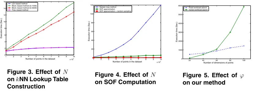
Effect ofNon constructing Full kNN Lookup Table.N

determines the length of the sorting lists obtained from the original dataset, which will further affect the efficiency of

kNN search of each point in constructing itskNN Lookup Table. In this experiment, the block sizebis set to be 1000 and 5000 for the block-based method and 1000 for the tree-based method (Note that the time complexity of tree-tree-based method is independent of the block size b). The time is averaged over 20 given points for all the methods. Fig-ure 3 presents the results. It shows that the list-based and tree-based methods are very close to each other in terms of running time and are more efficient than the block-based

method. This is because that the time complexities of list-based and tree-list-based methods are both logarithmic w.r.tN

while that of the block-based method is approximately lin-ear w.r.tN. Also, when block sizebis increased (say from 1000 to 5000 in this experiment), the complexity of the block-based method is decreased. In the extreme, when

b approachesN, the time complexity of the block-based method will becomeO(log2N+k), which will be equiv-alent to the complexities of the list-based and tree-based methods.

Effect ofNon SOF computation.Naffects the efficiency

of fitness evaluation for each subspace in the GA. When no approximation of SOF is used, the time complexity of fit-ness computation using the nested-loop method for kNN search is quadratic with respect to N. Nevertheless, the complexity can be reduced to a linear order ofN if our ap-proximation scheme of SOF is employed. Moreover, if we choose to work on the sampling data for performance boost, then the execution time is independent ofN in any way. This is because that the number of sampling points we use in fitness evaluation for subspaces is only depended on the characteristics of data, as revealed in Eq. (18). This empiri-cal analysis is confirmed in Figure 4. In this experiment, the execution time is the average time spent in evaluating each subspace. The results of this experiment illustrate that SOF approximation and sampling are very promising in boost-ing performance of our method. Under differentN values, our algorithm can run 2-20 times faster than the nested-loop method when using SOF approximation and can run 10-130 times faster when using both SOF approximation and ran-dom sampling.

Effect ofϕon the search workload of the GA.ϕ

1 2 3 4 5 6 7 8 9 10 x 104

0 2 4 6 8 10 12 14 16

Number of points in the dataset

Execution time (Sec.)

List−based method Block−based method (b=1000) Block−based method (b=5000) Tree−based method

Figure 3. Effect ofN onkNN Lookup Table Construction

1 2 3 4 5 6 7 8 9 10 x 104

0 20 40 60 80 100 120

Number of points in the dataset

Execution time (Sec.)

Nested−loop method SOF approximation SOF approximation + random sampling

Figure 4. Effect ofN on SOF Computation

20 40 60 80 100 0

1000 2000 3000 4000 5000 6000

Number of dimensions of points

Execution time (Sec.)

Fixed workload search Varied workload search

Figure 5. Effect of ϕ on our method

the varied workload scheme. The running time of these two search schemes for detecting SOF Outlying Subspaces of 20 given data points are presented in Figure 5. The running time of our algorithm under fixed workload scheme scales linearly w.r.tϕwhile that under varied workload scheme is in a quadratic order ofϕ.

7.2

Experimental Results on Real-life Datasets

Using the real-life multi- and high-dimensional datasets in UCI machine learning repository, we investigate the per-formance of our method in fitness convergence and sub-space refinement.

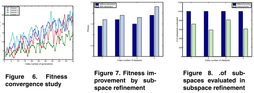
Fitness convergence study. GA tends to produce an

in-creasing number of fitter individuals as evolution proceeds, referring to as the phenomenon of convergence. In this ex-periment, we investigate the fitness convergence of our tech-nique. For each generation, the number of individuals with relatively high fitness (≥2.0) are counted. As we can see from Figure 6 that the number of individuals with high fit-ness for the four datasets is increased as the GA evolves, which indicates a good convergence of our method. A good convergence is beneficial as this will enable our method to find good outlying subspaces w.r.t the given point without exploring a huge number of subspaces.

Fitness boost by performing refinement in the GA. We

study the contribution of the subspace refinement step used in GA to enhancing fitness of the outlying subspaces de-tected, compared to the case when no refinement is in-volved. When no refinement is performed in the GA, the SOF Outlying Subspaces are the top n subspaces in the

CandidateSethaving the highest approximated SOF val-ues. However, there topnoutlying subspaces chosen based on approximated SOF values may not be the true outlying subspaces having the high SOF values. The fitness improve-ment by using the refineimprove-ment step is due to the extra com-putations performed on the subspaces inCandidateSetin order to get their accurate SOF values and the top n

sub-spaces with the highest accurate SOF values are returned as SOF Outlying Subspaces. Figure 7 presents the results. The results demonstrate that the fitness gain by performing the refinement step ranges from 13% and 21% for the four datasets when compared with the case when no refinement is performed.

Subspace pruning in refinement step of the GA.In this

experiment, we would like to study the advantage of em-ploying the subspace pruning strategy, devised based on the bounds of Dk, in computation saving in the refine-ment step of the GA. The bounds ofDk _{of subspaces help}

speed up our method by pruning away those subspaces in

CandidateSet that are definitely not relevant to the final SOF Outlying Subspace in the subspace refinement step. In this experiment, we set the number of subspaces in

CandidateSetas 1000 and compare it with the number of subspaces whose SOFs have actually been computed in the refinement step. From Figure 8, we can see that our prun-ing strategy is effective in greatly reducprun-ing the number of subspaces to be evaluated in the refinement step and such saving ranges from 19% to 41% for the four datasets.

8

Conclusions

0 5 10 15 20 25 30 35 40 45 50 0

5 10 15 20 25 30

Index number of generations

Number of subapces having high fitness

Dataset 1 Dataset 2 Dataset 3 Dataset 4

Figure 6. Fitness convergence study

1 2 3 4

0 0.5 1 1.5 2 2.5

Index number of datasets

Fitness

Without refinement With refinement

Figure 7. Fitness im-provement by sub-space refinement

1 2 3 4

0 200 400 600 800 1000 1200

Index number of datasets

# of subspaces evaluated

Without pruning Using pruning

Figure 8. .of sub-spaces evaluated in subspace refinement

the experimental results of our method on both synthetic and real-life datasets. The results demonstrate the efficiency and effectiveness of our method in handling outlying sub-space detection.

Acknowledgment

This research work is supported in part by research grant of Natural Sciences and Engineering Research Council of Canada (Grant No.: 312423).

References

[1] R. Agrawal, J. Gehrke, D. Gunopulos and P. Raghavan. Au-tomatic subspace clustering of high dimensional data for data mining applications.SIGMOD’98, pp 94-105, 1998.

[2] M. Breuning, H-P. Kriegel, R. Ng, and J. Sander. LOF: Iden-tifying Density-Based Local Outliers.SIGMOD’00, Dallas, Texas, pp 93-104, 2000.

[3] V. Barnett and T. Lewis.Outliers in Statistical Data. John Wiley, 3rd edition, 1994.

[4] L. Boudjeloud and F. Poulet. Visual Interactive Evolutionary Algorithm for High Dimensional Data Clustering and Outlier Detection.PAKDD’05, Hanoi, Vietnam, pp426-431, 2005.

[5] M. Ester, H-P. Kriegel, J. Sander, and X. Xu. A Density-based Algorithm for Discovering Clusters in Large Spa-tial Databases with Noise. SIGKDD’96, Portland, Oregon, USA, pp 226-231, 1996.

[6] D. Hawkins.Identification of Outliers. Chapman and Hall, London, 1980.

[7] A. Hinneburg, and D. A. Keim. An Efficient Approach to Cluster in Large Multimedia Databases with Noise.

SIGKDD’98, New York, NY, pp 58-65, 1998.

[8] W. Jin, A. K. H. Tung and J. Han. Finding Top n Local Out-liers in Large Database.SIGKDD’01, San Francisco, CA, pp 293-298, 2001.

[9] E. M. Knorr and R. T. Ng. Algorithms for Mining Distance-based Outliers in Large Dataset.VLDB’98, New York, NY, pp 392-403, 1998.

[10] E. M. Knorr and R. T. Ng. Finding Intentional Knowledge of Distance-based Outliers.VLDB’99, Edinburgh, Scotland, pp 211-222, 1999.

[11] R. Ng and J. Han. Efficient and Effective Clustering Methods for Spatial Data Mining.VLDB’94, Santiago, Chile, pp 144-155, 1994.

[12] S. Ramaswamy, R. Rastogi, and K. Shim. Efficient Al-gorithms for Mining Outliers from Large Data Sets. SIG-MOD’00, Dallas, Texas, pp 427-438, 2000.

[13] J. Tang, Z. Chen, A. Fu, and D. W. Cheung. Enhancing Ef-fectiveness of Outlier Detections for Low Density Patterns.

PAKDD’02, Taipei, Taiwan, 2002.

[14] J. Zhang and H. Wang. Detecting Outlying Subspaces for High-dimensional Data: the New Task, Algorithms and Performance. Knowledge and Information Systems(KAIS), Springer-Verlag Publisher, 2006.

[15] J. Zhang, W. Hsu and M. L. Lee. Clustering in Dynamic Spa-tial Databases. Journal of Intelligent Information Systems (JIIS)24(1): 5-27, Kluwer Academic Publisher, 2005.

[16] C. Zhu, H. Kitagawa and C. Faloutsos. Example-Based Robust Outlier Detection in High Dimensional Datasets.

ICDM’05, pp 829-832, 2005.

[17] C. Zhu, H. Kitagawa, S. Papadimitriou, and C. Faloutsos. OBE: Outlier by Example.PAKDD’04, pp 222-234, Sydney, Australia, 2004.

[18] J. Zhang, M. Lou, T. W. Ling and H. Wang. HOS-Miner: A System for Detecting Outlying Subspaces of High-dimensional Data.VLDB’04, pp 1265-1268, Toronto, Canada, 2004.

[19] T. Zhang, R. Ramakrishnan, and M. Livny. BIRCH: An Ef-ficient Data Clustering Method for Very Large Databases.