White Rose Research Online URL for this paper:
http://eprints.whiterose.ac.uk/114032/
Proceedings Paper:
Escolano, Francisco, Curado, Manuel, Biasotti, Silvia et al. (1 more author) (2017) Shape
Simplification Through Graph Sparsification. In: Graph-Based Representations in Pattern
Recognition - 11th IAPR-TC-15 International Workshop, GbRPR 2017, Anacapri, Italy, May
16-18, 2017, Proceedings. Springer Berlin / Heidelberg , pp. 13-22.
https://doi.org/10.1007/978-3-319-58961-9_2
[email protected] https://eprints.whiterose.ac.uk/
Reuse
Items deposited in White Rose Research Online are protected by copyright, with all rights reserved unless indicated otherwise. They may be downloaded and/or printed for private study, or other acts as permitted by national copyright laws. The publisher or other rights holders may allow further reproduction and re-use of the full text version. This is indicated by the licence information on the White Rose Research Online record for the item.
Takedown
If you consider content in White Rose Research Online to be in breach of UK law, please notify us by
Shape Simplification Through Graph
Sparsification
Francisco Escolano, Manuel Curado, Silvia Biasotti, and Edwin R. Hancock
Department of Computer Science and AI, University of Alicante, 03690, Alicante Spain
{sco,mcurado}@dccia.ua.es
CNR-IMATI, Via de Marini, 6 (Torre di Francia), 16149 Genova , Italy
Department of Computer Science, University of York, York, YO10 5DD, UK
Abstract. In this paper, we draw on Spielman and Srivastava’s method for graph sparsification in order to simplify shape representations. The underlying principle of graph sparsification is to retain only the edges which are key to the preservation of desired properties. In this regard, sparsification by edge resistance allows us to preserve (to some extent) links between protrusions and the remainder of the shape (e.g. parts of a shape) while removing in-part edges. Applying this idea to alpha shapes (abstract representations which have a huge number of edges) opens up a way of introducing a hierarchy of the edge strength, thus being relevant for shape analysis and interpretation.
Keywords: Graph sparsification, Shape simplification, Alpha shapes
1
Introduction
1.1 Shape representations: Triangulations vs Alpha shapes
an accurate and complex representation. Piecewise linear representations are at the center of the spectrum.
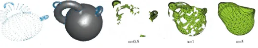
[image:3.595.179.440.334.383.2]The most popular representations in the piecewise class are the simplicial complexes [?], including triangular meshes that have become thede-facto stan-dard in graphics accelerators [?] and tetrahedral meshes that are used to rep-resent volumes and are used for the simulation of deformable models, such as organs or tissues. A generalization of the concept of triangulation are the so-called alpha (α-) shapes, that are families of piecewise linear simple curves in the Euclidean space associated with a dense and unorganized set of data points. An alpha shape is demarcated by a frontier, which is a linear approximation of the original shape. First introduced in the 2D plane by Edelsbrunner et al. [?], they were extended to 3D spaces [?] and higher dimensions [?]. In the case of 2D, an alpha shape consists of vertices, edges and triangles, while for 3D there are also tetrahedra. In our graph representation, we consider the 1-skeleton of both triangulations and alpha-shapes, i.e., the set of vertices and edges of the complex.
Fig. 1.From left to right: a point set, a triangulation and a sequence of three alpha shapes with increasing values ofα.
Alpha shapes depend on the parameterαused as radius of spheres centered on the points that determine the connection among the neighbourhoods. A very small value will generate many isolated points and the alpha shape degenerates to the point cloud when α → 0. On the other hand, a large value of α will consider many points inside the spheres and therefore the size of the 1-skeleton considerably increases. The limit of the alpha shape when α→ ∞ is the con-vex hull of the point cloud and the 1-skeleton of the alpha shape becomes the complete graph.
Shape and Sparsification 3
a large value ofαwill unfortunately close some handles. In practice, a large value of α results in (among possibly other things) a closure of handles, connection of multiple components and joints (e.g., sharp turns) being destroyed. For this reasons and because the general size of the 1-skeleton, the approach proposed in this work is able to simplify connections without destroying the global topology of the alpha shape.
1.2 Contributions
Spielman and Srivastava [?] have developed an efficient method for graph spar-sification based on edge resistance (which is proportional to the commute time of its end nodes). The method is based on the observation that the probability of an edge appearing in a random spanning tree of a graph is equal to its effec-tive resistance. Drawing on Spielman and Teng’s approximately linear solver[?], they show how to efficiently compute resistance, and hence sample edges for the purposes of sparsification.
Herein, we present a unified view of resistance sparsification through sam-pling. In addition, we exploit such a sampling for retaining edges (both in trian-gulations and alpha spaces) that are key to the preservation of the topological properties of the input shape. Our experiments show high compression rates as the allowed errorǫincreases. However each shape is sensitive to a different value of ǫ. It is the persistence of a given edge as ǫ increases what will provide us with is the relative importance of a vertex. This characterisation is pivotal for subsequent tasks such as efficient shape matching and shape representation.
2
Graph Sparsification
2.1 Definition and Ingredients
Graph sparsification [?] is the principled study of how to significantly decrease the number of edges of an input graphGso that the output,H, preserves some of the structural properties ofG.
Bencz´ur and Karger [?] showed that every cut inG= (V, E) can be approx-imated in H = (V, E′), withE′
⊆E, so that every cut in H has a value within (1±ǫ) times its value inG. For instance, aKn (complete) graph withnvertices andO(n2) edges can be approximated by a randomd
−regular graph, i.e. a graph withO(dn) edges. This means that for every subsetS⊂V the ratio between the value of a cut in Kn and that of the same cut in the random d−regular graph H isn/d. This link between sparsification and random graphs is useful (to some extent). For instance, if an edge in G is included in H with probabilty p, we must setp≫1/cwherecis the value of the minimal cut. As a result, if we have medges in Gwe can only haveO(m/c) edges inH.
ensures that the expected weight ofein H is unity.
Thechoice of a suitable value of pe is the first step in graph sparsification. For cut sparsification, the choice ofperelies on thestrongconnectivity ceof e. The strong connectivityceis the maximum value of a cut in a connected compo-nent includinge. This quantitiy is upper bounded by the standard connectivity ofe(the minimal value of a cut separating its endpoints), but it is hard to find. However lower bounds c′
e ≤ce can be founds through sparse certification (see details in [?]). In this way we have that pe =ρ/c′e≥ρ/ce, whereρis the com-pression factor, is a good choice forpe. Thecompression factorρhas complexity O(c(d+ 2)(logn)/ǫ2) and it is in turn inversely proportional to the squared error
ǫ2. The settingp
e = min{1, ρ/c′e} then ensures the correctness of the approxi-mation with probability 1−n−d.
The above rationale leads to the second ingredient of sparsification, namely theminimal number of samplesrequired to correctly sparsify the graph with high probability. For cut sparsification, we have that takingO(nρ), i.e.O(nlogn/ǫ2),
samples will suffice. This can be proved by means of the Chernoff bound, which is a standard information-theoretic tool for limiting the number of samples.
2.2 Spectral Formulation and Effective Resistances
An alternative approach to the the sparsification problem consists of enforcing the preservation of structural properties by bounding the quadratic form asso-ciated with the graph Laplacian of the sparsified graphH with respect to that of the input graphG(see the survey in [?]). Therefore, given G= (V, E, w) we must obtain H = (V, E′, w′) by taking O(nlogn/ǫ2) independent samples, so
that we satisfy (with probability at least 1/2) the following constraint
∀x∈Rn : (1−ǫ)≤xTLGx≤xTLHx≤(1 +ǫ)xTLG , (1)
where ǫ >0, n=|V|, and LG, LH are the respective Laplacian matrices ofG andH. Recall thatLG=D−W whereDis the diagonal degree matrix andW is the weighted adjacency matrix, and that xTL
Gx=P(u,v)∈E(x(u)−x(v))2wuv and similarly forLH.
Since Laplacian matrices are Semidefinite Positive (SDP), which is denoted byLG 0, we can reformulate Eq. 1 in terms of circumventing the hyper ellipsoid associated withLH with that associated withLG, i.e. one must satisfy
(1−ǫ)LGLH(1 +ǫ)LG, or equivalentlyLG LH κLG , (2)
with κ = 1+1−ǫǫ. This implies that all of the eigenvalues λ ′
i of LH satisfy λ′i ≤ κλi, whereλi is the corresponding eigenvalue ofLG. In addition, since Eq. 2 is invariant under rescaling, we have that
L−G1/2LGL −1/2
G L
−1/2
G LHL
−1/2
G κL
−1/2
G LGL −1/2
G (3)
i.e.
IL−G1/2LHL −1/2
Shape and Sparsification 5
whereIis the identity matrix andL−G1/2LHL −1/2
G is the so calledrelative
Lapla-cian. This leads to locatingLH so that the relative Laplacian is properly con-tained between I andκI. In this regard, the structure ofLH is determined by a weighted sum of outer products: LH =Pe∈Ew
′
ebebTe, where w ′
e are the un-known weights, be = δu−δv = buv, δu is the unit vector with a 1 at u and zeros elsewhere (similarly forv), ande= (u, v) is the edge. In this regard, since E′
⊆E, an edge ofEnot included inE′will havew′
e= 0. We define the random variables se (our unknowns) so that we′ =sewe whereE(se) = 1 for all e∈E. Then, Eq. 4 can be rewritten as follows
IL−G1/2 X e∈E
seweL −1/2
G bebTe !
L−G1/2κI . (5)
It is well known that the Laplacian matrixLcannot be inverted since it contains the zero eigenvalue. Expressions including the inverse must be computed using the pseudo-inverseL+ instead. The pseudo inverse plays a key role in defining
the effective resistance acrosse= (u, v) (the scaled commute time)Re, which is given by
Re= (δu−δv)TL+(δu−δv) =bTeL+be. (6) Then, combining Eqs. 5 and 6 we obtain
IX
e∈E
sewevevTe κI , (7)
whereve=L −1/2
G be, i.e., the squared norm ofveis
||ve||2= (L −1/2
G be)T(L −1/2
G be) = (bTeL −1/2
G )(L −1/2
G be) =bTeL+Gbe=Re. (8)
This squared norm allows us to treat P
e∈EsewevevTe in Eq. 5 as a quadratic form quite close to the identity matrix I. This is extremely important since: i) the relative Laplacian relies on the effective resistances ofG, and ii) we can pose the sparsification problem in terms of finding the sampling probabilities pe so that the constraint in Eq. 5 is satisfied. To this end, Batson et al. [?] exploited the following fact:
X
e∈E ˜
ve˜vTe =I , (9)
where ˜ve = w1e/2ve. This can be proved by using the m×n incidence matrix of G, i.e. B, with elements B(e, v) = 1 if v is e’s head, B(e, v) = −1 if v is e’s tail, and B(e, v) = 0 otherwise. Then the Laplacian matrix ofGis given by LG =BTWeB, whereWe is the diagonal m×m matrix where We(e, e) =we. Since the vectorsve=L
−1/2
G berely on the columns of BT, we have that vectors ˜
ve=vew1e/2are the columns of a n×mmatrix ˜V =L−G1/2BTWe1/2. Then
X
e∈E ˜
vev˜Te = ˜VV˜T =L −1/2
G B
TW1/2
e We1/2BL −1/2
G =L
−1/2
G LGL −1/2
In addition we have that
||˜ve||2= (w1e/2L −1/2
G be)T(w1e/2L −1/2
G be) =we(bTeL+Gbe) =weRe, (10) i.e. we obtain weighted effective resistances. The identity||v˜e||2=weResuggests to sampleE with probabilitiespe proportional toweRe.
Let y1, y2, . . . , yq vectors drawn independently with replacement from the distribution
y=√1 pe
˜
vewith probabilitype. (11)
Then, the expectation of yyT (which contains the effective resistances) is
EyyT
=X
e∈E pe
1 pe
˜
vev˜Te =I . (12)
In addition, the shape of each of theqsamplesyi = ˜ve/√pe leads to
1 q
q X
i=1
yiyiT = 1 q
q X
i=1
#e√v˜e pe ·
˜ vT e √p e = 1 q q X i=1
#e˜vev˜ T e pe
=X
e∈E
sev˜e˜veT , (13)
where #eis the number of times thateis sampled, andse= #e/qpe. Then, we obtain 1 q q X i=1
yiyTi = X
e∈E
se˜vev˜eT = X
e∈E
seweveveT , (14)
i.e. a proper sampling process leads to the relative Laplacian. This is ensured insofar 1
q Pq
i=1yiyTi andEyyT conform the Chernoff bound for matrices [?]:
E " 1 q q X i=1
yiyiT −E yyT #
≤min CM s
logq q ,1
!
, (15)
where || EyyT
|| < 1 and supy||y|| ≤ M. The first norm condition is verified sinceEyyT
=I. For verifying the second norm condition we must set the link betweenweRe(weighted effective resistances) andpe(sampling probabilities). In order to do so, Spielman and Srivastava [?] exploit the fact thatP
eweRe=n−1. Therefore, we may set
pe= weRe
n−1 so that ||y||= 1
√p
e p
weRe= r
n−1 weRe
p
weRe=√n−1. (16)
Therefore, takingq= 9C2nlogn/ǫ2 yields
E " 1 q q X i=1
yiyiT−E yyT # ≤C s
ǫ2log(9C2nlogn/ǫ2)(n−1)
9C2nlogn ≤ǫ/2, (17)
fornlarge enough andǫ≥1/√n.
Shape and Sparsification 7
1. Given the input graph G= (V, E, w), estimate the effective resistances Re for eache∈E.
2. Set an error tolerance ǫ. SetE′ =
∅,w′ =
∅, defineH = (V, E′, w′) and set #e= 0 for all edges inE.
3. Makeq= 9C2nlogn/ǫ2independent samples (with replacement) with
prob-abilitype∝weRe. Each sample is associated with an edgee.
4. Ifeis selected from a cumulative sum test, then increment #eand addeto E′ with weight 1/p
e. 5. For alle∈E′
set w′ e=
#e qpe.
Finally, the computationRecan be accomplished using exact spectral meth-ods [?]. However, this step takesO(n3) steps and the eigenvalues are ill
condi-tioned if the graphGhas several connected components. This is why Spielman and Srivastava [?] propose to approximate the computation of effective resis-tances by exploiting the Achlioptas version [?] of the Johnson-Lindenstrauss (JL) Lemma. This lemma states that if we project the original vectors (for in-stance those belonging to the effective resiin-stance embedding) onto a subspace spanned byO(logn) random vectors, the distances between the projected vec-tors and the original ones are preserved, and then to some extent are given by ǫ.
3
Experiments
We have performed several experiments on the reduction of the 1-skeleton of both triangulations and alpha shapes. As previously mentioned, triangulations are the standardde-facto representations of the surface of 3D objects.
Triangulations are sets of triangles and vertices and are fully described by their 1-skeleton. All vertices of a triangulation have the same importance. For instance, it is not possible to distinguish peaks, pits or passes from other struc-tures. Moreover, connections are all represented without any relations with their importance (for instance from shape outliers or dense regions). For this reason, it is necessary to derive more abstract, high level shapes. In this sense, spar-sification can act has a tool able to determine a hierarchy between the vertex connections. It may therefore determine a relative importance of the vertices.
Alpha shapes provide a family of shaperepresentations that is very useful when performing shape reconstruction. The reason for this is that they connect vertices with all neighbourhoods that are enclosed in a ball of radius alpha. In general, alpha shapes generalize triangulations and their importance is mainly theoretical. In our experiments on 3D point clouds, triangulations represent the external boundary connections, while alpha shapes encode spatial (volumetric) relationships.
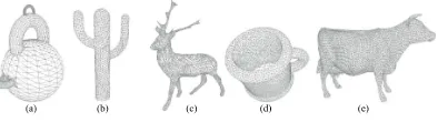
the elongated parts (in the cactus, the deer and the cup models). The results in Table 1 report the number of edges when sparsification is performed and how they vary when the value of theǫparameter increases1.
[image:9.595.161.449.325.398.2]Fig. 2.Examples of triangulations used in our experiments.
Table 1. Statistics on the number of edges of the 1-skeleton of some triangulations when the parameterǫincreases.
Triangulation ǫ= 0 ǫ= 0.25ǫ= 0.75ǫ= 1.25ǫ= 1.75ǫ= 2.25
Model in Fig. 2(a) 3906 3905 3837 3090 2098 1438 Model in Fig. 2(b) 4623 4622 4550 3643 2543 1782 Model in Fig. 2(c) 15012 15011 14757 11871 80623 5506 Model in Fig. 2(d) 18837 18836 18504 17146 10392 7290 Model in Fig. 2(e) 21759 21757 21415 17201 11677 7989
Similarly Fig. 3 shows the 1-skeletons of five alpha shapes that were con-structed over various point clouds, also varying the αvalue. These correspond to two different versions of the abstract shape already shown in 2(a), two alpha shapes of the deer model in 2(c) and an alpha shape from the cow point set that correspond to 2(e). The choice of these alpha shapes is motivated by the presence of small and larger handles and features that alpha shapes have diffi-culty capturing with a single choice of the parameterα, as previously discussed. The results in Table 2 report the number of edges of the 1-skeleton of the alpha shape when the value of the ǫparameter increases. From these experiment, we think that with sparsification would be possible to overcome the limitations of alpha shapes in the sense that we hope that it will be possible to commence from a quite large value of the parameters α and then to remove the redun-dant edges by using sparsification, thus implementing a connected, progressive, geometrical-topological peeling of the shape.
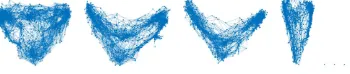
Finally, Fig. 4 shows the potential degradation of the topological properties of the simplified shape as ǫ increases. For the abstract shape (models (a),(b) in Fig. 3) we observe that the shape of the graph is preserved up to ǫ = 1.2. However, for ǫ= 1.25 the representation collapses to the most important
con-1 In this paper, the parameterǫcontrols the number of samples needed by the process,
Shape and Sparsification 9
Fig. 3.Examples of alpha shapes used in our experiments.
nected component. This is partially due to the fact that the link between the original resistances Re (ǫ= 0) and their sampled counterparts R′e is governed by R′
e = (1±ǫ)2Re according to the JL lemma, if we do not compute them by spectral means. In addition, as ǫincreases we reduce the number of samples q = 9C2nlogn/ǫ2 (C = 1 in this paper). This leads to an increment of
[image:10.595.220.395.352.389.2]en-tropy, which in turn flattens the importance of certain key edges. Therefore, the critical value of ǫ is larger for shapes with an increasing number of nodes. For instance, for the deer alpha shapes we have that the critical value ofǫis in the range [1.4,1.45] whereas for the cow alpha shape we have that it is in the range [1.4,1.5]. For triangulations the values are similar but larger. For the blob the critical value is close to 1.4, and for the remaining ones is the range [1.4,1.5].
Fig. 4.Degradation of topological properties asǫincreases. 2D projections of the blob
alpha shape. From left to right:ǫ= 0,ǫ= 0.75,ǫ= 1.0 andǫ= 1.25.
Table 2. Statistics on the number of edges of the 1-skeleton of some alpha shapes when the parameterǫincreases.
Alpha-shape α ǫ= 0 ǫ= 0.25ǫ= 0.75ǫ= 1.25ǫ= 1.75ǫ= 2.25
Model in Fig. 3(a) 3 8492 8491 6960 4167 2453 1621 Model in Fig. 3(b) 10 9526 9525 7643 4316 2563 1663 Model in Fig. 3(c) 1 39224 39223 33083 19476 11596 7531 Model in Fig. 3(d) 10 39707 39705 33416 19440 11664 7502 Model in Fig. 3(e) 10 55598 55596 48044 28769 17304 11235
4
Conclusions
[image:10.595.152.457.493.566.2]therefore a priority queue) of the edge strength. It is relevant for shape analysis and interpretation. We plan to further develop these ideas, in particular, in relation to the filtrations induced by the theory of topological persistence [?,?].
Acknowledgments. F. Escolano and M. Curado are funded by Project TIN2015-69077-P of the Spanish Government. E. Hancock is
References
1. Achlioptas, D.: Database-friendly random projections. In Buneman, P., ed.: Pro-ceedings of the Twentieth ACM SIGACT-SIGMOD-SIGART Symposium on Prin-ciples of Database Systems, PODS, May 21-23, 2001, Santa Barbara, California, USA, ACM (2001)
2. Batson, J.D., Spielman, D.A., Srivastava, N.: Twice-ramanujan sparsifiers. SIAM J. Comput.41(6) (2012) 1704–1721
3. Batson, J.D., Spielman, D.A., Srivastava, N., Teng, S.: Spectral sparsification of graphs: theory and algorithms. Commun. ACM56(8) (2013) 87–94
4. Bencz´ur, A.A., Karger, D.R.: Approximating s-t minimum cuts inO˜(n2) time. In: Proceedings of the Twenty-Eighth Annual ACM Symposium on the Theory of Computing, STOC, Philadelphia, Pennsylvania, USA, May 22-24, 1996. (1996) 47–55
5. Berger, M., Tagliasacchi, A., Seversky, L.M., Alliez, P., Guennebaud, G., Levine, J.A., Sharf, A., Silva, C.T.: A survey of surface reconstruction from point clouds. Computer Graphics Forum (2016) n/a–n/a
6. Edelsbrunner, H.: Alpha shapes - aurvey. In: Tessellations in the Sciences: Virtues, Techniques and Applications of Geometric Tilings. Springer Verlag (2011) 7. Edelsbrunner, H., Harer, J.: Computational Topology: An Introduction. American
Mathematical Society (2010)
8. Edelsbrunner, H., Kirkpatrick, D., Seidel, R.: On the shape of a set of points in the plane. IEEE Transactions on Information Theory29(4) (Jul 1983) 551–559 9. Edelsbrunner, H., Letscher, D., Zomorodian, A.: Topological persistence and
sim-plification. Discrete Comput. Geom.28(2002) 511–533
10. Edelsbrunner, H., M¨ucke, E.P.: Three-dimensional alpha shapes. ACM Trans. Graph.13(1) (January 1994) 43–72
11. Naylor, B., Bajaj, C., Edelsbrunner, H., Kaufman, A., Rossignac, J.: Computa-tional representations of geometry. SIGGRAPH’96 course notes. (1996)
12. Paoluzzi, A., Bernardini, F., Cattani, C., Ferrucci, V.: Dimension-independent modeling with simplicial complexes. ACM Trans. Graph. 12(1) (January 1993) 56–102
13. Qiu, H., Hancock, E.R.: Clustering and embedding using commute times. IEEE Trans. Pattern Anal. Mach. Intell.29(11) (2007) 1873–1890
14. Rudelson, M., Vershynin, R.: Sampling from large matrices: An approach through geometric functional analysis. J. ACM54(4) (July 2007)
15. Spielman, D.A., Srivastava, N.: Graph sparsification by effective resistances. SIAM J. Comput.40(6) (2011) 1913–1926
16. Spielman, D.A., Teng, S.: Spectral sparsification of graphs. SIAM J. Comput.