This is a repository copy of
Identifying the most informative features using a structurally
interacting elastic net
.
White Rose Research Online URL for this paper:
http://eprints.whiterose.ac.uk/132582/
Version: Accepted Version
Article:
Cui, Lixin, Bai, Lu, Zhang, Zhihong et al. (2 more authors) (2018) Identifying the most
informative features using a structurally interacting elastic net. Neurocomputing. pp. 1-14.
ISSN 0925-2312
https://doi.org/10.1016/j.neucom.2018.06.081
Reuse
This article is distributed under the terms of the Creative Commons Attribution-NonCommercial-NoDerivs (CC BY-NC-ND) licence. This licence only allows you to download this work and share it with others as long as you credit the authors, but you can’t change the article in any way or use it commercially. More
information and the full terms of the licence here: https://creativecommons.org/licenses/
Takedown
If you consider content in White Rose Research Online to be in breach of UK law, please notify us by
Identifying The Most Informative Features Using A
Structurally Interacting Elastic Net
Lixin Cui1∗, Lu Bai1∗, Zhihong Zhang2, Yue Wang2, Edwin R. Hancock3
1Central University of Finance and Economics, Beijing, China. 2Xiamen University, Xiamen, Fujian, China.
3University of York, York, UK.
Abstract
Feature selection can efficiently identify the most informative features with respect to
the target feature used in training. However, state-of-the-art vector-based methods are
unable to encapsulate the relationships between feature samples into the feature
selec-tion process, thus leading to significant informaselec-tion loss. To address this problem, we
propose a new graph-based structurally interacting elastic net method for feature
selec-tion. Specifically, we commence by constructing feature graphs that can incorporate
pairwise relationship between samples. With the feature graphs to hand, we propose
a new information theoretic criterion to measure the joint relevance of different
pair-wise feature combinations with respect to the target feature graph representation. This
measure is used to obtain a structural interaction matrix where the elements represent
the proposed information theoretic measure between feature pairs. We then formulate
a new optimization model through the combination of the structural interaction matrix
and an elastic net regression model for the feature subset selection problem. This
al-lows us to a) preserve the information of the original vectorial space, b) remedy the
information loss of the original feature space caused by using graph representation,
and c) promote a sparse solution and also encourage correlated features to be
select-ed. Because the proposed optimization problem is non-convex, we develop an efficient
alternating direction multiplier method (ADMM) to locate the optimal solutions.
Ex-tensive experiments on various datasets demonstrate the effectiveness of the proposed
∗These authors contribute equally to this work and are co-first authors. Correspondence author: Lu Bai,
method.
Keywords: Feature Selection; Graph; Interacting Elastic Net; Sparse; ADMM
1. Introduction
There has recently been a rapid growth in both the size and dimension of the
da-ta encountered in many real world applications of pattern recognition including
im-age processing, bioinformatics, and financial analysis. Finding useful information and
building effective prediction models from such data presents new challenges for ma-5
chine learning and pattern recognition [1]. One way to overcome this problem is to
de-velop efficient spectral methods including stochastic neighbour embedding [2], elastic
embedding methods [3] and feature selection [4] methods to reduce the dimensionality
of the data.
Feature selection aims to identify an optimal subset of the most informative fea-10
tures by removing irrelevant and redundant features [4]. One of the main advantages is
that feature selection can improve the predictive accuracy and enhance
comprehensi-bility of learning tasks [5]. Unlike feature extraction, feature selection can maintain the
properties of the original features and has better interpretability. This is very important
for understanding which features are most informative with respect to the target feature 15
used in training. For instance, in Peer-to-Peer (P2P) lending analysis, it is important
to understand which features of the P2P lending platforms (e.g., operation time,
reg-istered capital, and management team) affect the investors’ decisions [6]. For medical
diagnosis, it is crucial to know which characteristics of the patients (e.g., age, gender,
and weight) affect the occurrence of a certain disease [7]. 20
Because of these advantages, many efficient feature selection methods have been
developed [5] [8]. Existing feature selection algorithms can be broadly categorized as
filter and wrapper methods depending on whether the learning algorithm is used in the
feature subset selection process [9]. Filter methods utilize the intrinsic properties of
the data to build quantitative evaluation criteria [10]. By contrast, wrapper methods 25
[11] evaluate the selected feature subsets based on the performance measures of the
better than filter methods, they require significantly higher computational costs. In
addition, in the presence of redundant features, wrappers tend to locate suboptimal
subsets, and the characteristics of the selected subset are inevitably biased depending 30
on the choice of the classifier [9]. Therefore, for high-dimensional data, filter methods
are often preferred [12].
To construct effective filter methods, a good evaluation criterion is necessary. To
date, many evaluation criteria have been used, including correlation [13],
consisten-cy [14], Fisher score [15], and mutual information (MI) [16]. For instance, MI 35
measures the mutual dependence of two variables [16] and has been shown to have
similar or better performance than other more sophisticated methods [17]. Due to its
excellent performance, MI has received considerable attention for developing various
information theoretic feature selection methods. Representative examples include 1)
the Mutual Information-Based Feature Selection (MIFS) [18], 2) the MIFS method 40
under the assumption of a uniform distribution of input variables (MIFS-U) [19], 3)
the Maximum-Relevance Minimum-Redundancy criterion (MRMR) [20], and 4) the
Normalized Feature-Feature Mutual Information method (NMIFS) [21]. Although the
performance of MI-based feature selection methods have been demonstrated in many
applications, they suffer from two widely acknowledged limitations. First, they require 45
the number of selected features to be predetermined. Second, they adopt greedy search
methods to identify the most informative feature subsets [22]. To overcome these
short-comings, Liu et al. [23] have proposed the adaptive MI-based feature selection method
that automatically determines the number of most informative features, by maximizing
the average pairwise informativeness. Zhang and Hancock [24] have developed a hy-50
pergraph based information theoretic feature selection method that can automatically
determine the size of the most informative feature subset through dominant hypergraph
clustering [25].
However, none of the aforementioned information theoretic feature selection
meth-ods can incorporate pairwise relationship between samples of each feature dimension. 55
More specifically, assume a dataset withNfeatures denoted asX ={f1, . . . ,fi, . . . ,fN},
and each featurefi hasM samples asfi = (fi1, . . . , fia, . . . , fib, . . . , fiM)T.
vec-tor, and thus ignore the relationship between pairwise samplesfiaandfib infi. This
deficiency restricts the precision of the information theoretic measure between pairs 60
of features. To address this drawback, Cui et al. [26] have recently developed a new
feature selection method using graph-based features. Specifically, they transform each
feature vector into a graph structure that encapsulates pairwise relationship between
samples. The most relevant vectorial features are located by selecting the graph-based
features that are most similar to the graph-based target feature, in terms of the Jensen-65
Shannon divergence measure between the graphs. To adaptively determine the most
relevant feature subset, Cui et al. [27] have further developed a new information
theo-retic feature selection method which a) encapsulates the relationship between sample
pairs for each feature dimension and b) automatically identifies the subset containing
the most informative and least redundant features by solving a quadratic programming 70
problem.
However, the aforementioned graph-based feature selection methods may lead to
significant information loss concerning the relationships between samples from the
o-riginal vector space. To illustrate this point, assume that two pairs of samples from
the same feature dimensionfi are denoted as{fi1, fi3}and{fi3, fi5}, respectively.
75
Following Cui et al. [27], we transform the feature vectorfiinto a graph-based
repre-sentationGi, which is a complete weighted graph. Each vertexva ofGi represents
a corresponding samplefiainfi and each weighted edge(va, vb)represents the
rela-tionship between sample pairfiaandfib. If the Euclidean distances of the two pairs,
i.e.,{fi1, fi3} and{fi3, fi5} are the same, the weights associated with the two pairs
80
of samples are also the same in the feature graphGi. However, these two pairs of
samples are located differently in the original vector space. This means that the
graph-based feature representation may lead to information loss. One exception is that the
vertex label is the associated sample value of the original features, i.e., the vertex label
is continuous. However, in this case, we need to measure the affinity between a pair of 85
graphs associated with continuous vertex labels and this results in significantly higher
computational complexity [28].
To summarize the above, it is fair to say that it still remains a challenge to develop
pairwise relationship between samples of each feature dimension and avoid informa-90
tion loss from the original vector space.
On the other hand, sparse feature selection methods have received increasing
at-tention [29]. By formulating feature selection as a regression model with an ordinary
least square (OLS) term and a specifically designed sparsity inducing regularizer, the
regression model can be efficiently represented by a linear combination of a set of the 95
most active variables. The cardinality of the set of the selected variables is significantly
smaller than the entire number of variables [30]. In other words, the regression model
retains information concerning the original feature space and also allows us to
adap-tively select the most informative feature subset. Because of these advantages, many
efficient regularization techniques including Lasso [31], Elastic Net [32], and Group 100
Lasso [33] have been extensively studied for high-dimensional data feature selection.
For instance, Zheng and Liu [7] have developed a Lasso operator to identify the most
informative features for cancer classification, where Lasso enforces automatic feature
selection by forcing at least some features to zero. Panagakis et al. [34] have developed
a new similarity measure based on the matrix Elastic Net regularization to efficiently 105
deal with highly correlated audio feature vectors. Marafino et al. [35] have proposed
an efficient sparse feature selection method for biomedical text classification using the
Elastic Net. More recently, Zhang et al. [30] have devised a new regularization term in
the Lasso regression model to impose high order interactions between covariates and
responses. The high-order relations among covariates are represented by a feature hy-110
pergraph and then used as a regularizer on the covariate coefficients to automatically
select the most relevant features.
Although sparsity is desirable for designing effective feature selection algorithms,
it is worth noting that most of the existing sparse feature selection methods seldom
consider pairwise relationship between samples from each feature dimension. Intu-115
itively, such structural information is important for improving the efficiency of feature
selection methods. In addition, as opposed to the Elastic Net, the use of Lasso proves
to be problematic when at least some features are highly correlated. In this case, Lasso
selects one feature at random. As a result, givenntraining samples, Lasso can only
Motivated by the above discussion, we aim to overcome the limitations of
exist-ing feature selection methods by developexist-ing a novel structurally interactexist-ing elastic net
feature selection method. The proposed method not only considers the structural
re-lationships between feature samples but also remedies the information loss caused by
the graph-based representation of features. In addition, we also explore how to ensure 125
sparsity and promote a grouping effect among selected features via elastic net
regular-ization.
1.1. Related Work
Feature selection has been widely studied in machine learning and pattern analysis.
The topic of feature selection has been reviewed in a number of recent papers [36], [37] 130
and [38]. In this section, we briefly state-of-the-art MI-based and sparse feature
selec-tion methods, which are related to our proposed method.
MI is often considered as an evaluation criterion to measure the relevance between
features and the target labels due to its effectiveness at quantifying how much
informa-tion is shared by two random variables. Because of this, MI has been extensively used 135
for developing information theoretic feature selection methods. In the earlier reported
work, Battiti [18] introduced a first order incremental search algorithm based on MI
known as the MIFS criterion,
JM IF S =I(fi;C)−β ∑
fs∈S
I(fs;fi). (1)
For a given set of existing selected featuresS, at each step MIFS locates the
candi-date featurefiwhich maximizes the relevance to the classI(fi;C), instead of
calculat-ing the joint MI between the selected features and the class labelC. The proportional
termβI(fs;fi)measures the overlap information between the candidate feature and
existing features, and is used to regulate the feature selection process. The parameterβ
may significantly influence the features selected and needs to be carefully controlled.
It is worth noting that because MIFS only considers features that have maximum MI
with the output classes, it might treat features that have rich information about the
Kwak and Choi [19] improved MIFS by developing MIFS-U under the assumption of
a uniform distribution for selected features. This uniform criterion is defined as
JM IF S−U =I(fi;C)−β
∑
fs∈S
I(fs;C)
H(fs)
I(fi;fs), (2)
whereH(fs) = −∑
fs∈SP(fslogP(fs))is the entropy associated with the
proba-bility distribution forfs. Instead of calculatingI(C;fi|S)directly, onlyI(S;fi)and 140
I(C;fi)are computed. The conditional MI (denoted asI(C;fi|S)) between the class
labelCand the candidate featurefifor a given feature subsetScan be approximated
asI(C;fi|S) =I(C;fi)−I(S;fi)−I(S;fi|C).
Although MIFS-U gives better estimation than MIFS, the model parameters need to
be carefully controlled to avoid bad results. To overcome this problem, Peng et al. [20]
proposed a parameter-free method, referred to as MRMR, which is defined as
JM RM R=I(fi;C)− 1
|S|
∑
fs∈S
I(fi;fs), (3)
where|S|is the cardinality of the selected feature setS. MRMR uses the average of
the redundancy term to eliminate the difficulty of parameter selection ofβwith MIFS
and MIFS-U methods. However, as a first-order incremental method, that
sequential-ly selects one feature after another based on the evaluation function, MRMR presents
similar limitations as MIFS and MIFS-U in the presence of many irrelevant or
redun-dant features. This is because the conditional MII(C;fi|S)between the target class
Cand the candidate featurefifor a given subset of featuresSis ignored. To deal with
this problem, Estevez et al. [21] developed the normalized NMIFS method to achieve
a balance between the relevance and the redundancy term, defined as
JN M IF S=I(fi;C)−
1 |S|
∑
fs∈S
ˆ
I(fi;fs), (4)
whereIˆ(fi;fs) = I(fifs)
inf(H(fs),H(fi)) is the normalized MI.
On the other hand, sparse feature selection methods have recently attracted much
attention. Typically we have a set of training data{(xi, yi), i = 1, ..., N}, which is
used to estimate the regression coefficientsβ. Eachxi= (f1i, f2i, ..., fdi)T ∈Rd×1is a
model, the most popular ordinary least square (OLS) method is adopted. OLS selects
the coefficientsβ = (β1, ..., βd)T by minimizing the residual sum of squares denoted
as
min
β∈ℜd
N ∑
i=1
∥yi− d ∑
j=1
βjfji∥22= min
β∈ℜd∥y
T−βtX∥2 2
s.t. N ∑
i=1
∥β∥0=k, (5)
wherey∈ ℜN×1is the label (response) vector,X∈ ℜd×N is the training dataset,k
is a predetermined number of selected features. The minimisation of Eq.(5) has been
proved to be a NP-hard optimization problem and is very difficult to be solved. In
practice, we can relax the constraint equation by imposing a positive regularization
parameterλand adding it to the objective function, that is
min
β∈ℜd∥y
T−βtX∥2
2+λ∥β∥0. (6)
Unfortunately solving Eq.(6) is still challenging. Therefore, an alternative
formu-lation usingl1-norm regularization instead ofl0-norm has been proposed for practical
purposes. This corresponds to the regularized counterpart of the Lasso (least absolute
shrinkage and selection operator) problem in statistical learning [31]. Lasso imposes a
l1constraint on the regression coefficients, so that some of the regression coefficients
in the regression model will shrink to zeros. Thus it can automatically select a set of
the informative variables. Correspondingly, the feature selection problem with Lasso
penalty is defined as
min
β∈ℜd∥y
T−βtX∥2
2+λ∥β∥1, (7)
where∥β1∥is thel1-norm of vectorβ, that is,∥β1∥=∑dj=1|βj|. The parameterλ≥0 145
controls the amount of regularization applied to the estimate. The largerλ, the larger
the number of zeros inβ. The nonzero components give the selected variables. After
the optimal value ofβis obtained, one can choose the feature indices corresponding to
the topklargest values of the summation of the absolute values among each column.
Lasso requires the independence assumption of the input variables, however, in
correlated features, Lasso tends to select only one of these features at random, resulting
in suboptimal performance (37). Moreover, thel1minimization algorithm is not stable
when compared withl2 minimization (30). For this reason, the elastic net (5) adds
an additionall2 regularization term into the Lasso objective function, which can be
formulated as
min
β ∥y
T −βtX∥2
2+λ1∥β∥1+λ2∥β∥22, (8)
whereλ1, λ2≥0are the tuning parameters.
150
Elastic Net can be seen as a linear combination of the Lasso and Ridge penalty.
Whenλ1 = 0, it becomes simple Ridge regression, whenλ2 = 0, it is equivalent
to the Lasso penalty. Thus, Elastic Net enjoys a similar sparsity of representation of
Lasso and also allows groups of correlated features to be selected. In the literature, it
is reported that Elastic Net usually outperforms Lasso when the number of features is 155
much larger than the number of samples [32].
In summary, most of the exiting MI-based feature selection methods aim to develop
an efficient quantitative evaluation criterion that simultaneously maximizes relevancy
and minimizes redundancy. Unfortunately, it has been noted that such MI-based feature
selection methods have two common limitations. First, they tend to ignore pairwise 160
relationship between samples of each feature dimension, which leads to significant
information loss. Second, the majority of these methods cannot adaptively identify the
most informative feature subset. Alternatively, sparse feature selection methods like
Lasso and Elastic Net ensure parameter vector sparsity and allow the relevant features
to be adaptively selected. However, existing sparse feature selection methods also 165
fail to encapsulate pairwise relationship between samples for each feature dimension.
These drawbacks motivate us to develop a novel structurally interacting elastic net
feature selection method to adaptively locate the most informative feature subset.
1.2. Contributions
As previously stated, the aim of this paper is to overcome the limitations of exist-170
ing MI-based and sparse feature selection methods by developing a new structurally
this work are threefold. First, we transform each vector feature into a graph-based
ture representation, where each vertex represents a corresponding sample in each
fea-ture dimension and each weighted edge represents the pairwise relationship between 175
samples from each feature dimension. We use the Euclidean distance to measure the
pairwise relationship between samples. Similarly, we also construct a complete
fea-ture graph for the target feafea-ture. To measure the joint relevance of different pairwise
feature combinations with respect to the target feature, we propose a new information
theoretic criterion using the Jensen-Shannon divergence (JSD). Based on this criteria, 180
we obtain a new interaction matrix which characterizes the informative relationships
between feature pairs. Second, to a) incorporate the pairwise sample relationships in
each feature dimension, b) remedy information loss in the original feature space, and
c) adaptively select the most informative feature subset, we formulate the proposed
graph-based feature selection method as an elastic net regression model. Specifically, 185
the interaction matrix encapsulates high-dimensional structural relationships between
feature samples and thus provides richer representation of structural interaction
infor-mation between features. The ordinary least-square (OLS) term utilizes inforinfor-mation
from the original feature space, and thus remedies the information loss caused by
rep-resenting features as graphs. In addition, thel1-norm regularizer ensures sparsity in
190
the coefficients of variables and thel2-norm regularizer promotes a grouping effect to
select correlated features. Third, an efficient alternating direction multiplier method
(ADMM) is presented to solve the proposed elastic net optimization problem.
Com-prehensive experiments on eight standard machine learning datasets and two publically
available datasets demonstrate the effectiveness of the proposed method. 195
1.3. Paper Outline
The remainder of the paper is organized as follows. Section 2 discusses the
impor-tant concepts which will be used for the proposed feature selection method. Section 3
presents the proposed structurally interacting elastic net for feature selection. Section 4
2. Preliminary Concepts
In this section, we review some preliminary concepts that will be used in this work.
We commence by reviewing how to construct the feature graph to incorporate structural
information for feature samples. Then we introduce the concept of Jensen-Shannon
divergence, which will be used to calculate the similarity between feature graphs. 205
2.1. Construction of Feature Graphs
In this subsection, we introduce how to transform each vectorial feature into a
com-plete weighted graph. The advantages of using the graph-based representation are
t-wofold. First, graph structures have a stronger ability to encapsulate global topological
information than vectors. Second, graphs can incorporate the relationships between 210
samples of each original vector feature into the feature selection process, thus reducing
information loss.
Given a dataset ofN features denoted asX ={f1, . . . ,fi, . . . ,fN} ∈ RM×N,fi represents thei-th vectorial feature and hasMsamplesfi= (fi1, . . . , fia, . . . , fib, . . . , fiM)T.
We transform each feature fi into a graph-based feature representation Gi(Vi, Ei), 215
where the vertexvia∈Viindicates thea-th samplefiaoffi. Each pair of verticesvia
andvibare connected by a weighted edge(via, vib)∈Ei, and the dissimilarity weight
ω(via, vib)of(via, vib)is the Euclidean distance betweenfiaandfib, i.e.,
ω(via, vib) =
√
(fia−fib)2. (9)
Similarly, if the sample values of the target featureY= (y1, . . . , ya, . . . , yb, . . . , yM)T
are continuous, its graph-based feature representationGˆ( ˆV ,Eˆ)can be computed
us-ing Eq.(9) and the vertexvˆa represents thea-th sampleya. However, for
classifica-tion problems, the target featuresY are the class labels and thus takes the discrete
valuesc ∈ {1,2, . . . , C}, i.e., the samples of each feature fi are assigned to theC
different classes. In this case, we propose to compute the graph-based target feature
ˆ
Gi( ˆVi,Eiˆ )for each featurefi, where the dissimilarity weightω(ˆvia,vibˆ )of each edge
(ˆvia,ˆvib)∈Eiˆ is
ω(ˆvia,ˆvib) =
√
whereµiais the mean value of all samples infifrom the same classc.
2.2. The Jensen-Shannon Divergence
220
In information theory, the JSD is a dissimilarity measure between probability
dis-tributions. Let two (discrete) probability distributions beP = (p1, . . . , pa, . . . , pA)
andQ= (q1, . . . , qb, . . . , qB), then the JSD betweenP andQis defined as
JSD(P,Q) =HS(P+Q
2
)
−1
2HS(P)− 1
2HS(Q), (11)
whereHS(P) =∑Aa=1palogpais the Shannon entropy of the probability distribution
P. In [39], the JSD has been used as a means of measuring the information
theoret-ic dissimilarity between graphs associated with their probability distributions. In this
work, we are concerned with the similarity between graph-based feature
representa-tions. Therefore, we adopt the negative exponential ofJSD(P,Q)to compute the
similarity measureISbetween probability distributions, i.e.,
IS(P,Q) = exp{−JSD(P,Q)}. (12)
3. The Proposed Feature Selection Method
In this section, we introduce our proposed structurally interacting elastic net feature
selection method. We first detail the formulation of the structurally interacting elastic
net model. To solve the optimization model, the alternating direction method of
multi-plier (ADMM) algorithm [40] is used to identify the most informative feature subset. 225
Finally, we provide the convergence proof and complexity analysis for the method.
We propose to use the following information theoretic criterion to measure the joint
relevance of different pairwise feature combinations with respect to target labels. For a
set ofNfeaturesf1, . . . ,fi, . . . ,fj, . . . ,fNand the associated continuous target feature
Y, the relevance degree of the feature pair{fi,fj}is
Wfi,fj =
IS(Gi,Gˆ) +IS(Gj,Gˆ)
IS(Gi,Gj)
, (13)
whereGiandGˆare the graph-based feature representations offiandY,ISis the JSD
measure consists of three terms. The first and second termsIS(Gi,Gˆ)andIS(Gj,Gˆ)
are the relevance degrees of individual features fi andfj with respect to the target 230
featureY, respectively. The third termIS(Gi,Gj)measures the relevance between
the feature pair{fi,fi}. Therefore,Wfi,fj is large if and only if bothIS(Gi,Gˆ)and
IS(Gj,Gˆ)are large (i.e., bothfi andfj are informative themselves with respect to
the target feature representationY) andIS(Gi,Gj)is small (i.e., fi andfj are not
relevant). 235
For classification problems, the samples of the target featureY take the discrete
valuecandc ∈ {1,2, . . . , C}. In this case, we compute the individual graph-based
target feature representationGˆifor each featurefi, and the relevance measure defined
in Eq.(13) can be written as
Wfi,fj =
IS(Gi,Gˆi) +IS(Gj,Gˆj)
IS(Gi,Gj)
. (14)
Similarly to Eq.(13), the three terms of Eq.(14) have the same corresponding
theo-retical significance.
Furthermore, based on the graph-based feature representations, we construct a
fea-ture informativeness matrixW, where each elementWi,j ∈ Wrepresents the
infor-mation theoretic measure between a feature pair{fi,fj}based on Eq.(13) (for Yis
continuous) or Eq.(14) (forYis discrete). Given the informativeness matrixWand
the d-dimensional feature indicator vectorβ, whereβi represents the coefficient for
the i-th feature, we can identify the informative feature subset by solving the following
maximization problem
maxf(β) = max
β∈ℜdβ
TWβ,
(15)
subject toβ ∈RN,β≥0. The solution vectorβ = (β1, ..., βd)Tto the above
quadrat-ic program is anN-dimensional vector. Whenβi > 0, thei-th featurefibelongs to
the most informative feature subset i.e., featurefi is selected if and only if thei-th 240
component ofβis positive (i∈ {1,2, ..., d}).
3.1. The Proposed Structurally Interacting Elastic Net
The proposed feature subset selection algorithm aims to incorporate structural
be selected, as well as promote a sparse solution. Therefore, we combine Eq.(15) and
Eq.(8) to construct the associated structurally interacting elastic net for feature
selec-tion with the following mathematical form
min
β∈ℜd
1 2∥y
T−βTX∥2
2+λ1∥β∥1+λ2∥β∥22−λ3βTWβ, (16)
whereλ1andλ2are the tuning parameters in the elastic net regression model, andλ3
is the associated tuning parameter for the structural interaction matrixW.
It can be seen that the first term in Eq.(16) remedies the information loss from 245
the original feature space, while the second and third terms ensure the sparsity and
grouping among selected features. The fourth term incorporates structural
informa-tion concerning the relainforma-tionships between feature samples. BecauseβTWβ is a
non-convex constraint, the proposed method distinguishes itself from existing Lasso-type
methods using convex optimization methods, which may become trapped in subopti-250
mal solutions. Specifically, for the proposed model (16), we need to develop efficient
algorithms to obtain the optimal solutions (denoted asβ∗). A featurefiis selected if
and only ifβ∗i >0. Consequently, we can recover the number of features in the optimal
feature subset according to the number of positive components ofβ∗.
3.2. Optimization Algorithm
255
To solve the non-convex problem (16), we develop an optimization algorithm
us-ing ADMM [40]. The ADMM approach is a powerful algorithm that is well suited to
problems arising in machine learning. The basic principle of the ADMM approach is
to decompose a hard optimization problem into a series of smaller ones, each of which
is simpler to handle. It takes the form of a decomposition-coordination procedure, in 260
which the solutions to small local subproblems are coordinated to find a solution to a
large global problem. ADMM can be viewed as an attempt to blend the benefits of
dual decomposition and augmented Lagrangian methods for constrained optimization.
It turns out to be equivalent or closely related to many well known algorithms as well,
such as Douglas-Rachford splitting from numerical analysis [41], proximal method-265
In ADMM form, problem (16) can be re-written as
min
β∈ℜd
1 2∥y
T −βTX∥2
2+λ2∥β∥22−λ3βTWβ+λ1∥γ∥1
s.t. β−γ= 0, (17)
whereγis an auxiliary variable, which can be regarded as a proxy for vectorβ. By
doing so, the objective function can be split into two separate parts associated with two
different variables, i.e.,βandγ, indicating that the hard constrained problem can be
solved separately. As in the method of multipliers, we form the augmented Lagrangian
function associated with the constrained problem (16) as follows
Lρ(β, γ, z) =
1 2∥y
T−βTX∥2
2+λ2∥β∥22−λ3βTWβ+λ1∥γ∥1+< β−γ, z >+
ρ
2∥β−γ∥ 2 2,
(18)
where⟨·,·⟩is an Euclidean inner product,zis a dual variable (i.e.,the Lagrange
multi-plier) associated with the equality constraintβ =γ, andρis a positive penalty
param-eter (step size for dual variable update). By introducing an additional variableγand an
additional constraintβ−γ= 0, we have simplified the optimization problem (16) by 270
decoupling the objective function into two parts that depend on two different variables.
In other words, ADMM decomposes the minimization ofLρ(β, γ, z)into two simpler
subproblems. Specifically, ADMM solves the original problem (16) by seeking for a
saddle point of the augmented Lagrangian by iteratively minimizingLρ(β, γ, z)over
β,γ, andz. In ADMM, the variablesβ,γ, andzare updated in an alternating or se-275
quential fashion, which accounts for the term alternating direction. This updating rule
is shown below
(1)βk+1= arg min
β∈ℜdL(β, γk, zk), //β-minimization
(2)γk+1= arg min
β∈ℜdL(βk+1, γ, zk), //γ-minimization
(3)zk+1=zk+ρ(βk+1−γk+1), //z-update
280
Given the above updating rule, we need to resolve each sub-problem iteratively
until the termination criteria is satisfied. Using ADMM, we perform the following
calculation steps at each iteration.
(a)Updateβ
sub-problem, where the values ofγkandzkare fixed
min
β∈ℜd
1 2∥y
T−βTX∥2
2+λ2∥β∥22−λ3βTWβ+λ1∥γ∥1+< β−γk, zk>+
ρ
2∥β−γ
k∥2 2.
(19)
Let the partial derivative with respect toβbe equal to zero, we have
∂[minβ∈ℜd 1
2∥y
T −βTX∥2
2+λ2∥β∥22−λ3βTWβ+λ1∥γ∥1+< β−γk, zk>+ρ2∥β−γk∥22]
∂β = 0,
(20) because
∂(1 2∥y
T−
βTX∥2 2)
∂β =−Xy+XXTβ
∂(λ2∥β∥22)
∂β =λ2β
∂(−λ3βTWβ)
∂β =−2λ3Wβ
∂<β−γk,zk>
∂β =z
k
∂(ρ2∥β−γk∥2 2)
∂β =ρ(β−γ
k),
(21)
we have
−Xy+XXTβ+λ2β−2λ3Wβ+zk+ρ(β−γk) = 0, (22)
that is,
βk+1= (XXT +λ2I−2λ3W+ρI)−1(Xy−zk+ργk). (23)
(b)Updateγ 285
Based on the results, assumeβki+1andzk
i are fixed, fori = 1,2, ..., d, we update
γik+1by solving the following sub-optimization problem
min γi λ1 d ∑ i=1
∥γi∥1−
d ∑
i=1
< γi, zik >+
ρ
2
d ∑
i=1
∥βik+1−γi∥22, (24)
∂[minγiλ1
∑d
i=1∥γi∥1−∑id=1< γi, zik >+ρ2
∑d
i=1∥βk +1
i −γi∥22]
∂γi
= 0. (25)
We therefore have the following results
γki+1=
1
ρ(zik+ρβk
+1
i −λ1), ifzik+ρβk
+1
i > λ1
1
ρ(zik+ρβk
+1
i −λ1), ifzik+ρβk
+1
i <−λ1
0, ifzk
i +ρβk
+1
i ∈[−λ1, λ1]
(c)Update z
Then, assumeβki+1andγik+1are fixed, fori= 1,2, ..., d, we updatezik+1by using
the following equation
zik+1=zki +ρ(βik+1−γik+1). (27)
Based on procedures (a), (b), and (c), we summarize the optimization algorithm
below
Algorithm 1The proposed ADMM algorithm for structurally interacting Elastic Net.
Input:X,y, β0 , z0
, λ1, λ2, λ3, ρ
Step1: While(not converged),do Step2:Updateβk+1
according to Eq.(23)
Step3:Updateγik+1, i= 1,2, ..., daccording to Eq.(26) Step4:Updateβk+1
i , i= 1,2, ..., daccording to Eq.(27) End While
Output:β∗.
3.3. Complexity Analysis and Convergence Proof
290
In this subsection, we provide an analyses of the properties of the proposed
struc-turally interacting elastic net method. We commerce by presenting the computational
complexity which is followed by a convergence analysis.
3.3.1. Analysis of Computational Complexity
LetN be the number of features,M the number of samples, andK the required 295
number of iterations to converge. At each iteration, the computational complexity for
updatingβ according to Eq.(23) isO(N2M). Additionally, the computational costs
for updatingγin Eq.(26) andzin Eq.(27) are bothO(N). Therefore, the overall time
complexity of the ADMM algorithm is calculated asmax{O(N2M K), O(M K)}.
3.3.2. Convergence Proof
300
To theoretically prove the convergence of the proposed ADMM algorithm, we
Theorem 1. Assume the iterative sequences generated by the ADMM algorithm
are denoted as{βk},{γk},and{zk}, respectively. Suppose asktends to infinity, the
sequence{zk}converges to a pointz′, that is,lim
k→∞zk=z′. Following this, every
305
limit point(β′, γ′)of the iteration sequence {βk, γk}, together with z′, satisfy the
necessary first order conditions of the problem (16), that is
(1)Primal feasibility, i.e.,β′−γ′ = 0.
(2)Dual feasibility, i.e.,∇f(β′) +z′= 0and0∈∂g(γ′)−z′, where∂denotes the
sub-differential operator. 310
We can easily proveTheorem 1by following a proof similar to that of Proposition
3 in Magn´usson[43]. We can conveniently draw the conclusion fromTheorem 1that,
in general, the ADMM algorithm converges to a local optimum solution to problem
(16), that is,(β′, γ′, z′) = (β∗, γ∗, z∗).
4. Experimental Results and Discussion 315
In this section, we conduct a series of experiments to demonstrate the performance
of the proposed structurally interacting elastic net feature selection method
(InElas-ticNet). A comprehensive experimental study on two types of datasets is conducted
to validate its effectiveness and make comparison with several state-of-the-art feature
selection methods. 320
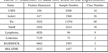
4.1. Experiments on Standard Machine Learning Datasets
Two categories of public datasets are used in our experiment, including eight
wide-ly used machine learning (ML) datasets and two public available datasets. The ML
datasets are the USPS handwritten digit data set [44], Isolet speech data set and Pie
data set from the UCI Machine Learning Repository [45], YaleB face data set [46], 325
Lymphoma and Leukemia datasets [47], BASEHOCK and RELATHE. Note that the
last two datasets are both large in feature dimension and sample size. Detailed
infor-mation for these data sets are summarized in Table 1.
To evaluate the discriminative capabilities of the information captured by our method,
Table 1: Statistics of data sets used in the experiments Name Feature Dimension Sample Number Class Number
USPS 256 9298 10
Isolet1 617 1560 26
Pie 1024 11554 68
YaleB 1024 2414 38
Lymphoma 4026 96 9
Leukemia 7129 73 2
BASEHOCK 4862 1993 2
RELATHE 4322 1427 2
posed method with several state-of-the-art feature selection methods including
Las-so [31], ULasLas-so [48], Fused LasLas-so [49], Elastic Net [32], Group LasLas-so [33],
InLas-so [30], and one graph-based feature selection methods, namely, GF-RW [27].
a) Lasso [31]: As a typical sparse feature selection method, Lasso performs feature
selection through thel1-norm, where features corresponding to zero coefficients in the
335
parameter vector will be discarded.
b) ULasso [48]: The uncorrelated Lasso (ULasso) aims to conduct variable
de-correlation and variable selection simultaneously, so that the variables selected are
un-correlated as much as possible.
c) Fused Lasso [49]: The fused lasso enforces sparsity in both the coefficients and 340
their successive differences. It is desirable for applications with features ordered in
some meaningful way.
d) Group Lasso [33]: The group Lasso is known to enforce the sparsity on variables
at an inter-group level, where variables from different groups are competing to survive.
e) Elastic Net [32]: In statistics, the elastic net is a regularized regression method 345
that linearly combines thel1 andl2penalties of the Lasso and Ridge methods. This
ensures democracy among groups of correlated groups and allows selection of the
rel-evant groups while simultaneously promoting sparse solutions for feature selection.
f) InLasso [30]: Is a Lasso-type regression model which incorporates high-order
feature interactions, InLasso can effectively evaluate whether a feature is redundant 350
or interactive based on a neighborhood dependency measure. This method can avoid
discarding some valuable features arising in individual feature combinations.
g) GF-RW [27]: Is a graph-based feature selection method which incorporates
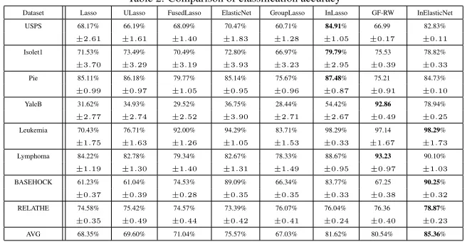
Table 2: Comparison of classification accuracy
Dataset Lasso ULasso FusedLasso ElasticNet GroupLasso InLasso GF-RW InElasticNet
USPS 68.17% 66.19% 68.09% 70.47% 60.71% 84.91% 66.99 82.83%
±2.61 ±1.61 ±1.40 ±1.83 ±1.28 ±1.05 ±0.17 ±0.11
Isolet1 71.53% 73.49% 70.49% 72.80% 66.97% 79.79% 75.53 78.82%
±3.70 ±3.29 ±3.19 ±3.93 ±3.23 ±2.95 ±0.39 ±0.33
Pie 85.11% 86.18% 79.77% 85.14% 75.67% 87.48% 75.21 84.73%
±0.99 ±0.97 ±1.05 ±0.95 ±0.96 ±0.87 ±0.91 ±0.10
YaleB 31.62% 34.93% 29.52% 36.75% 28.44% 54.42% 92.86 78.94%
±2.77 ±2.74 ±2.52 ±3.90 ±2.71 ±2.67 ±0.49 ±0.25
Leukemia 70.43% 76.71% 92.00% 94.29% 83.71% 98.29% 97.14 98.29%
±1.75 ±1.63 ±1.26 ±1.05 ±1.53 ±0.33 ±1.67 ±1.73
Lymphoma 84.22% 82.78% 79.34% 82.67% 78.33% 88.67% 93.23 90.10%
±1.19 ±1.30 ±1.40 ±1.31 ±1.49 ±0.95 ±0.97 ±1.03
BASEHOCK 61.23% 61.04% 74.53% 89.09% 66.34% 83.77% 67.25 90.25%
±0.37 ±0.39 ±0.28 ±0.35 ±0.35 ±0.33 ±0.38 ±0.32
RELATHE 74.58% 75.42% 74.57% 73.39% 76.07% 76.04% 76.36 78.87%
±0.35 ±0.49 ±0.44 ±0.42 ±0.41 ±0.24 ±0.40 ±0.23
AVG 68.35% 69.60% 71.04% 75.57% 67.03% 81.62% 80.54% 85.36%
Generally, we adopt a 10-fold cross-validation method associated with C-SVM to 355
evaluate the classification accuracy. To be specific, we first partition the entire sample
randomly into 10 subsets (each subset with roughly equal size) and then we choose one
subset for testing and use the remaining 9 subsets for training. We repeat this procedure
for 10 times. The final accuracy is computed by averaging of the accuracies from all
10 experiments and we also compute the associated standard error. 360
Fig. 1 shows the classification accuracy versus the number of selected features on
the datasets for different methods. It is clear from the figure that the proposed method
InElasticNet is, by and large, superior to the following alternative feature selection
methods including Lasso, ULasso, Elastic Net, Fused Lasso, and Group Lasso on all
datasets. When compared with InLasso, it is clear that our method significantly outper-365
forms InLasso on the YaleB dataset and also outperforms InLasso for BASEHOCK and
RELATHE, which are challenging datasets both large in feature dimension and sample
size. For the remaining datasets, our method is competitive to InLasso. In addition,
our method significantly outperforms GF-RW method on USPS, Pie and BASEHOCK,
and is superior than GF-RW on Isolet1, Leukemia, and RELATHE datasets. As Fig. 1 370
shows, when the number of selected features is too small, the advantage of our method
is not clear. However, when the number of total features in the selected subset increases
alterna-0 5 10 15 20 25 30 35 40 45 50 Number of features
0 0.1 0.2 0.3 0.4 0.5 0.6 0.7 0.8 0.9 1 Classification accuracy YaleB GF-RW Lasso ULasso FusedLasso ElasticNet GroupLasso InLasso InElasticNet
(a) YaleB dataset
0 5 10 15 20 25 30 35 40 45 50 Number of features
0 0.1 0.2 0.3 0.4 0.5 0.6 0.7 0.8 0.9 1 Classification accuracy USPS GF-RW Lasso ULasso FusedLasso ElasticNet GroupLasso InLasso InElasticNet
(b) USPS dataset
0 10 20 30 40 50 60 70 80 90 100 Number of features
0 0.1 0.2 0.3 0.4 0.5 0.6 0.7 0.8 0.9 1 Classification accuracy Isolet1 GF-RW Lasso ULasso FusedLasso ElasticNet GroupLasso InLasso InElasticNet
(c) Isolet1 dataset
0 20 40 60 80 100 120 140 160 180 200 Number of features
0 0.1 0.2 0.3 0.4 0.5 0.6 0.7 0.8 0.9 1 Classification accuracy lymphoma GF-RW Lasso ULasso FusedLasso ElasticNet GroupLasso InLasso InElasticNet
(d) Lymphoma dataset
0 10 20 30 40 50 60 70
Number of features 0 0.1 0.2 0.3 0.4 0.5 0.6 0.7 0.8 0.9 1 Classification accuracy Pie GF-RW Lasso ULasso FusedLasso ElasticNet GroupLasso InLasso InElasticNet
(e) Pie dataset
0 20 40 60 80 100 120 140 160 180 200 Number of features
0 0.1 0.2 0.3 0.4 0.5 0.6 0.7 0.8 0.9 1 Classification accuracy Leukemia GF-RW Lasso ULasso FusedLasso ElasticNet GroupLasso InLasso InElasticNet
(f) Leukemia dataset
0 20 40 60 80 100 120 140 160 180 200 Number of features
0 0.1 0.2 0.3 0.4 0.5 0.6 0.7 0.8 0.9 1 Classification accuracy BASEHOCK GF-RW Lasso ULasso FusedLasso ElasticNet GroupLasso InLasso InElasticNet
(g) BASEHOCK dataset
0 20 40 60 80 100 120 140 160 180 200 Number of features
0 0.1 0.2 0.3 0.4 0.5 0.6 0.7 0.8 0.9 Classification accuracy RELATHE GF-RW Lasso ULasso FusedLasso ElasticNet GroupLasso InLasso InElasticNet
(h) RELATHE dataset
[image:22.612.144.466.117.729.2]tive methods. The results verify that the proposed structurally interacting Elastic Net
can identify more informative feature subsets than the state-of-the-art feature selection 375
methods. Although the total numbers of features in the selected feature subsets are
on average slightly larger than those obtained via Lasso, it is still small as compared
to the total number of features in the datasets. This is because our method can select
correlated features and also encourage a sparse solution, whereas Lasso tends to select
only one feature from a group of correlated features, which may decrease its accuracy. 380
To make a detailed comparison, we report the mean classification accuracies and
corresponding variances (i.e.,MEAN±STD) obtained via various methods on each
da-ta set with different number of features selected by using the C-SVM classifier in
Ta-ble 2. The mean classification accuracy is obtained by averaging the accuracy achieved
via C-SVM using the largest number of features indicated in the corresponding sub-385
figures of Fig. 1 for each data set. For instance, for the YaleB dataset, we use the top
10, 20,...,50 features selected by each algorithm. The boldfaced value of each row
cor-responds to the highest accuracy obtained by the different methods for the underlying
dataset. Our proposed method, i.e., InElasticNet improves the classification accuracy
by 24.52% for the YaleB dataset and 1.43% for the Lymphoma dataset, respectively. 390
For the Leukemia dataset, InElasticNet performs equally to InLasso, and is better than
the alternative methods. As for Isolet1, USPS, and Pie, InElasticNet can obtain better
classification accuracy than Lasso, ULasso, FusedLasso, Elastic Net, and Group Lasso,
and is competitive to InLasso, which retains the highest classification accuracy.
Addi-tionally, for the two large datasets Basehock and Relathe, InElasticNet outperforms all 395
the competitors.
The bottom row of Table 2 displays the average classification accuracy for each
algorithm over the eight datasets. It shows that our proposed method, i.e., InElasticNet
improves the classification accuracy by 17.11%(Lasso), 15.57%(ULasso),
15.75%(Fus-edLasso), 11.93%(ElasticNet), 19.98%(GroupLasso), 3.36%(InLasso), and 4.82%(GF-400
RW), respectively, compared to the averaged classification accuracy of all alternative
methods on the eight datasets. In addition, it is worth noting that the standard errors for
the proposed InElasticNet method are smaller than the competing methods for almost
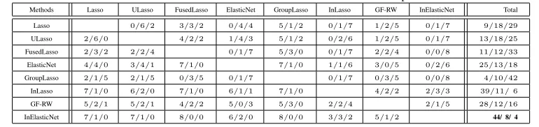
Table 3: Win/Tie/Lost matrix for the feature selection methods used in the experiments.
Methods Lasso ULasso FusedLasso ElasticNet GroupLasso InLasso GF-RW InElasticNet Total
Lasso 0/6/2 3/3/2 0/4/4 5/1/2 0/1/7 1/2/5 0/1/7 9/18/29
ULasso 2/6/0 4/2/2 1/4/3 5/1/2 0/2/6 1/2/5 0/1/7 13/18/25
FusedLasso 2/3/2 2/2/4 0/1/7 5/3/0 0/1/7 2/2/4 0/0/8 11/12/33
ElasticNet 4/4/0 3/4/1 7/1/0 7/1/0 1/1/6 3/0/5 0/2/6 25/13/18
GroupLasso 2/1/5 2/1/5 0/3/5 0/1/7 0/1/7 0/3/5 0/0/8 4/10/42
InLasso 7/1/0 6/2/0 7/1/0 6/1/1 7/1/0 4/2/2 2/3/3 39/11/6
GF-RW 5/2/1 5/2/1 4/2/2 5/0/3 5/3/0 2/2/4 2/1/5 28/12/16
[image:24.612.131.532.259.348.2]InElasticNet 7/1/0 7/1/0 8/0/0 6/2/0 8/0/0 3/3/2 5/1/2 44/ 8/ 4
Table 4: The best result of all methods and the corresponding size of selected feature subset
Dataset USPS Isolet1 Pie YaleB Leukemia Lymphoma BASEHOCK RELATHE
Lasso 86.30%(50) 91.67%(100) 94.48%(70) 46.64%(50) 82.86%(120) 94.44%(160) 66.33%(200) 86.00%(200)
ULasso 83.24%(50) 92.18%(100) 94.57%(70) 47.43%(50) 82.86%(200) 91.11%(200) 67.30%(200) 84.62%(200)
FusedLasso 87.40%(50) 88.08%(90) 93.53%(70) 55.89%(50) 98.57%(20) 94.44%(160) 84.62%(200) 86.50%(200)
ElasticNet 87.43%(50) 90.00%(100) 86.94%(70) 48.09%(50) 98.57%(180) 90.00%(120) 91.76%(200) 77.95%(180)
GroupLasso 83.93%(50) 83.53%(100) 92.35%(70) 45.02%(50) 91.43%(180) 91.11%(200) 73.33%(200) 74.16%(200)
InLasso 93.94%(50) 91.92%(100) 96.58%(70) 71.20%(50) 100%(80) 95.56%(140) 86.58%(200) 80.70%(180)
GF-RW 85.79%(50) 84.80%(100) 90.64%(70) 98.38%(50) 98.57%(20) 95.56%(160) 74.22%(200) 76.36%(180)
InElasticNet 94.10%(50) 92.23%(100) 96.81%(70) 94.62%(50) 100%(120) 95.56%(160) 92.75%(200) 83.66%(180)
the competing methods. 405
Table 3 presents the Win/Tie/Lost matrix for the feature selection methods used in
the experiments. The(i, j)th element of the matrix represents the number of datasets
where the method corresponding to theith row has won/tied/lost against the method
corresponding to thejth column. A tie is defined as a dataset on which difference in
classification accuracy between two methods is not statistically significant. The last 410
column of Table 3 shows the total number of wins/ties/lost for a given method, and
the best performing method is highlighted in bold. InElasticNet has the largest total
number of wins and the smallest total number of lost. This clearly indicates that the
proposed InElasticNet method performs significantly better than the alternative feature
selection methods. 415
Table 4 shows the best results for each competing method together with their
corre-sponding number of features in the selected subset. In the table, the best classification
accuracy is shown which is followed by the optimal number of features selected in
brackets. From this table, it is clear that the proposed method achieves the highest
classification accuracy using same number of features in the selected subset as the al-420
all the competing methods and has more discriminative power.
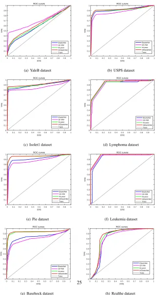
The ROC curves of the most competitive methods (ElasticNet, GF-RW, InLasso
and InElasticNet) on the eight datasets are plotted in Figure 2. From this figure, we
observe that except for the YaleB dataset, the proposed InElasticNet method achieves 425
superior performance to the competitors on all datasets. In summary, the
aforemen-tioned experimental results demonstrate that our proposed feature selection method
outperforms the alternative methods on the standard ML datasets.
4.2. Experiments on Two Real World Datasets
Apart from the ML datasets, two publically available datasets including i) a Peer-to-430
Peer (P2P) dataset collected from the P2P lending sector in China and ii) a healthcare
dataset collected from a well-known medical platform is used to validate the
effective-ness of the proposed feature selection approach.
Since the launch of the first P2P lending platform in 2007, the P2P lending
indus-try has developed rapidly and the market is enormous. Specifically, the total number of 435
operational P2P lending platforms nationwide has reached 2,448 with an accumulative
loan amount of 20 trillion yuan by the end of year 2016. Along with this rapid
de-velopment, the P2P lending industry has also experienced some serious problems with
rising defaults and weak risk control. Therefore, it is of great significance to develop
an effective decision aid for the credit risk analysis of P2P platforms. However, the 440
P2P lending data are often high-dimensional, highly correlated and unstable.
There-fore, it presents a challenge for traditional statistical pattern recognition and machine
learning techniques. The aim is to effectively analyze the data and identify which
fac-tors influence the performance of the lending platforms, or the default probability of
the borrowers, etc. To realize these goals, the sample relationships of the P2P data that 445
encapsulates significant information should be incorporated into the feature selection
process. However, the majority of existing feature selection methods ignore the sample
relationships and may cause significant information loss. By contrast, our proposed
structurally interacting feature selection approach is able to encapsulate the sample
0 0.1 0.2 0.3 0.4 0.5 0.6 0.7 0.8 0.9 1 FPR 0 0.1 0.2 0.3 0.4 0.5 0.6 0.7 0.8 0.9 1 TPR ROC curves ElasticNet GF-RW InLasso InElasticNet Trace
(a) YaleB dataset
0 0.1 0.2 0.3 0.4 0.5 0.6 0.7 0.8 0.9 1 FPR 0 0.1 0.2 0.3 0.4 0.5 0.6 0.7 0.8 0.9 1 TPR ROC curves ElasticNet GF-RW InLasso InElasticNet Trace
(b) USPS dataset
0 0.1 0.2 0.3 0.4 0.5 0.6 0.7 0.8 0.9 1 FPR 0 0.1 0.2 0.3 0.4 0.5 0.6 0.7 0.8 0.9 1 TPR ROC curves ElasticNet GF-RW InLasso InElasticNet Trace
(c) Isolet1 dataset
0 0.1 0.2 0.3 0.4 0.5 0.6 0.7 0.8 0.9 1 FPR 0 0.1 0.2 0.3 0.4 0.5 0.6 0.7 0.8 0.9 1 TPR ROC curves ElasticNet GF-RW InLasso InElasticNet Trace
(d) Lymphoma dataset
0 0.1 0.2 0.3 0.4 0.5 0.6 0.7 0.8 0.9 1 FPR 0 0.1 0.2 0.3 0.4 0.5 0.6 0.7 0.8 0.9 1 TPR ROC curves ElasticNet GF-RW InLasso InElasticNet Trace
(e) Pie dataset
0 0.1 0.2 0.3 0.4 0.5 0.6 0.7 0.8 0.9 1 FPR 0 0.1 0.2 0.3 0.4 0.5 0.6 0.7 0.8 0.9 1 TPR ROC curves ElasticNet GF-RW InLasso InElasticNet Trace
(f) Leukemia dataset
0 0.1 0.2 0.3 0.4 0.5 0.6 0.7 0.8 0.9 1 FPR 0 0.1 0.2 0.3 0.4 0.5 0.6 0.7 0.8 0.9 1 TPR ROC curves ElasticNet GF-RW InLasso InElasticNet Trace
(g) Basehock dataset
0 0.1 0.2 0.3 0.4 0.5 0.6 0.7 0.8 0.9 1 FPR 0 0.1 0.2 0.3 0.4 0.5 0.6 0.7 0.8 0.9 1 TPR ROC curves ElasticNet GF-RW InLasso InElasticNet Trace
(h) Realthe dataset
[image:26.612.143.465.123.725.2]The P2P dataset is collected from a reputable P2P lending portal in China1, which
tracks the industry. The dataset consists of the most popular 200 platforms (i.e., 200
samples) until Aug 2014. For each platform, we collect 19 features including 1)
trans-action volume, 2) total turnover, 3) average annualized interest rate, 4) the total number
of borrowers, 5) the total number of investors, 6) the online time, which refers to the 455
foundation year of the platform, 7) the operation time, i.e., number of months since the
foundation of the platform, 8) registered capital, 9) weighted turnover, 10) average
ter-m of loan, 11) average full ter-mark titer-me, i.e., tender period of a loan raised to the required
full capital, 12) average amount borrowed, i.e., average loan amount of each
success-ful borrower, 13) average amount invested, which is the average investment amount of 460
each successful investor, 14) loan dispersion, i.e., the ratio of the repayment amount
to the total capital, 15) investment dispersion, the ratio of the invested amount to the
total capital, 16) average times of borrowing, 17) average times of investment, 18) loan
balance, and 19) popularity.
We evaluate the performance of the proposed feature selection approach with re-465
spect to continuous target features. Specifically, we use the proposed method to
per-form credit risk evaluation of the P2P lending platper-forms. As it is difficult to obtain
sufficient data for the platforms which encountered a problem, we use the annualized
average interest rate as an indicator of the credit risk of the P2P lending platforms. In
finance, interest rate is the amount charged, expressed as a percentage of principal, by 470
a lender to a borrower for the use of assets. When the borrower is a low-risk party,
they will usually be charged a low interest rate. On the other hand, if the borrower
is considered high risk, the interest rate charged will be higher. Likewise, a higher
annualized average interest rate of the P2P lending platforms often indicates a greater
likelihood of default, i.e., higher credit risk of the platforms. Identifying the features 475
most relevant to the interest rate can help investors effectively manage the credit risks
involved in P2P lending. Therefore, in our experiment, we set the average annualized
interest rate as the target feature which takes continuous values. Our aim is to identify
the most informative subset of features for the credit risk of the P2P platforms by
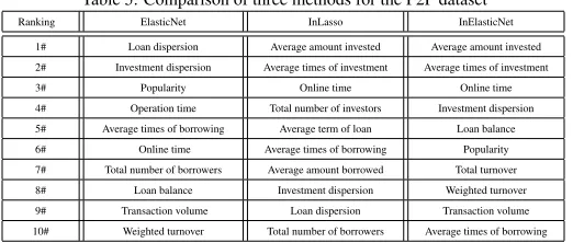
Table 5: Comparison of three methods for the P2P dataset Ranking ElasticNet InLasso InElasticNet
1# Loan dispersion Average amount invested Average amount invested
2# Investment dispersion Average times of investment Average times of investment
3# Popularity Online time Online time
4# Operation time Total number of investors Investment dispersion
5# Average times of borrowing Average term of loan Loan balance
6# Online time Average times of borrowing Popularity
7# Total number of borrowers Average amount borrowed Total turnover
8# Loan balance Investment dispersion Weighted turnover
9# Transaction volume Loan dispersion Transaction volume
10# Weighted turnover Total number of borrowers Average times of borrowing
ing the proposed feature selection method. To further strengthen our findings, we also 480
compare the proposed feature selection method with two alternative methods including
Elastic Net [32] and Interacted Lasso [30].
Table 5 presents a comparison of the results obtained using the competing methods.
For each method, we display the top 10 features in terms of relevance to the average
annualized interest rate. It is worth noting that all three methods can identify some 485
similar influential factors but differ from each other in the remaining factors. For
in-stance, both InLasso and InElasticNet rankthe average amount invested, average
times of investment, andonline timeas the top three most influential factors. This is
reasonable because a longer online time indicates that the P2P platform is in operation
for a relatively longer period of time, and is less risky. Moreover, a larger average 490
amount invested and a higher level of the average times of investment indicate a
high-er prefhigh-erence of the investors for the P2P lending platform due to a highhigh-er degree of
security. In addition, both methods considerinvestment dispersionas a relevant
fea-ture but with different rankings, i.e., the 4th for InElasticNet and the 8th for InLasso.
This is reasonable because investment dispersion is highly correlated with the average 495
amount invested and the average times of investment. Therefore, when InElasticNet
ranks these factors high, it also tends to rank investment dispersion high. This implies
that our proposed method can encourage a grouping effect for highly correlated
fea-tures. This is further demonstrated by the fact thatthe rankings of popularity (6th),
total turnover(7th), andweighted turnover (8th)are close to each other. Moreover,
500
these three factors are also correlated to each other. Whereas for InLasso, when groups
InLasso may fail to recognize some highly relevant features.
When compared to ElasticNet, it is worth noting that although both Elastic Net and
the proposed method (InElasticNet) can identifyonline time, popularity,weighted 505
turnover,transaction volume,average times of borrowing, andinvestment
disper-sionas influential factors, their rankings are quite different. This meets our
expecta-tions because both ElasticNet and InElasticNet can promote a grouping effect.
Howev-er, as InElasticNet utilizes the structural information between pairwise feature samples,
the results obtained are more encouraging. For instance, ElasticNet ranksloan disper-510
sion (1st)andinvestment dispersion (2nd)as the most influential factors whereas
InElasticNet ranksthe average amount investedas the highest andthe average times
of investmentas the second highest. Unfortunately, a higher level of loan dispersion
and investment dispersion does not necessarily correspond to a safer P2P platform with
a lower annualized interest rate. By contrast, a larger average amount invested and a 515
higher level of the average times of investment often indicate a higher preference of the
investors for the P2P lending platform due to a higher degree of security and a lower
level of annualized interest rate. These results demonstrate the effectiveness of the
pro-posed method for identifying the most influential factors for credit risk of P2P lending
platforms. 520
The healthcare dataset is collected from a well-known medical platform in China2,
which presents evaluation of doctors. The dataset consists of 2363 doctors (i.e., 2363
samples). For each doctor, we collect 13 features including 1) patients, i.e., total
num-ber of patients treated, 2) title, i.e., title of the doctor, 3) grade, i.e.,recommended grade
of the doctor provided by the website, 4) notes, i.e., total number of notes of thanks 525
posted by the patients, 5) gifts, i.e., total number of gifts received, 6) outpatients, i.e.,
total number of outpatients of the doctor, 7) city, i.e., city of the doctor, 8)appointments,
i.e., total number of appointments received from the patients, 9) visits, i.e., total
num-ber of visits of the doctor’s personal website, 10) contribution value, i.e., contribution
value of the doctor, 11) posts, total number of posts published by the patients about the 530
doctor, 12) votes, i.e., total number of votes received from the patients for a doctor, and
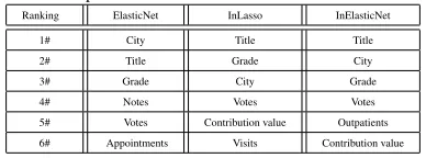
Table 6: Comparison of three methods for the healthcare dataset Ranking ElasticNet InLasso InElasticNet
1# City Title Title
2# Title Grade City
3# Grade City Grade
4# Notes Votes Votes
5# Votes Contribution value Outpatients
6# Appointments Visits Contribution value
13) registration fee for the doctor.
We use the proposed feature selection method to evaluate the doctors. The
regis-tration fee is treated as the continuous target and we aim to identify which features are
the most informative ones with respect to the target. Like for the P2P lending analysis, 535
we also compare the proposed feature selection method with two alternative methods
including Elastic Net [32] and Interacted Lasso [30].
Table 6 presents a comparison of the results obtained using the three methods. For
each method, we display the top 6 features in terms of relevance to the registration
fee. It is worth noting that all three methods can identifytitle of the doctor, city 540
locatedandgrade of the doctoras the top three most influential factors. However,
the rankings of these factors are different. For instance, both InLasso and InElasticNet
ranktitle of the doctorthe first, but ElasticNet ranks this factor as second. Compared
with InLasso, our method considerscityas the second most influential factor whereas
InLasso ranksGradeas the second. We believe the results obtained via our method 545
is more reasonable because a doctor with a higher title and in bigger cities are more
expensive. Although grade is also relevant to the registration fee of the doctor, it is not
an objective evaluation criteria. In addition, both InLasso and InElasticNet considerthe
number of votesas the fourth highest influential factor. This is also reasonable because
a greater number of votes received from the patients indicates a higher reputation of 550
the doctor. An interesting finding is that only our method can identifyoutpatientsas
the top ranking features whereas the two competing methods considerappointments
andvisits as the most influential features. We believe outpatients is a more relevant
feature to the registration fee of the doctor because a higher number of outpatients
often indicate that more patients are willing to pay more to be treated by the doctor. In 555
method can select the highly correlated features.
5. Conclusion
The main goal of feature selection is to automatically identify a subset of the most
informative features that is small in size but high in classification accuracy. To realize 560
this goal, in this paper, we have developed a new structurally interacting elastic net
feature selection method. The major contributions of this paper are threefold. First,
the proposed method can encapsulate structural relationships between feature samples
into the feature selection process by representing features as graphs and samples as
graph vertices. Accordingly, the informativeness matrix obtained is used to construct 565
an optimization model to identify the features with maximum relevancy and minimum
redundancy to the target feature. Second, to remedy the information loss caused by
using graph-based feature representations, we formulate the feature selection problem
using an elastic net regression model and solve this model using ADMM. This allows
us to a) incorporate information from the original feature space, b) reduce the number 570
of features to a small size and c) promote grouping effects. The experimental results on
real datasets show that our method outperforms several well-known feature selection
methods.
We plan to extend our method in a number of ways. First, in this paper, the
con-structed feature graphs are complete weighted graphs. However, in real world appli-575
cations, not all connections may be dominant and useful. In other words, the
com-plete weighted graphs may contain some noise. Therefore, one may want to define
a sparser graph. Second, in our previous work [50], we have developed a number
of quantum Jensen-Shannon kernels using both the continuous-time and discrete-time
quantum walks. It would be interesting to extend the proposed feature selection method 580
using the classical Jensen-Shannon divergence to that using its quantum counterpart.
Finally, the proposed feature selection method only considers the relationships between
pairwise features, i.e., it only evaluates the two-order relationships between features.
Our future work will extend the proposed method into a high-order feature selection