Three Essays on Corruption

(1)

2017

Three Essays on Corruption

Sumi Sharma

Follow this and additional works at: https://researchrepository.wvu.edu/etd

Recommended Citation Recommended Citation

Sharma, Sumi, "Three Essays on Corruption" (2017). Graduate Theses, Dissertations, and Problem Reports. 6620.

https://researchrepository.wvu.edu/etd/6620

This Dissertation is protected by copyright and/or related rights. It has been brought to you by the The Research Repository @ WVU with permission from the rights-holder(s). You are free to use this Dissertation in any way that is permitted by the copyright and related rights legislation that applies to your use. For other uses you must obtain permission from the rights-holder(s) directly, unless additional rights are indicated by a Creative Commons license in the record and/ or on the work itself. This Dissertation has been accepted for inclusion in WVU Graduate Theses, Dissertations, and Problem Reports collection by an authorized administrator of The Research Repository @ WVU. For more information, please contact [email protected].

(2)

Sumi Sharma

Dissertation submitted

to the College of Business and Economics at West Virginia University

in partial fulfillment of the requirements for the degree of

Doctor of Philosophy in Economics

Shuichiro Nishioka, Ph.D., Chair Brian Cushing, Ph.D. Stratford Douglas, Ph.D. Eugene Bempong Nyantakyi, Ph.D.

Daniel Berkowtiz, Ph.D. Department of Economics

Morgantown, West Virginia 2017

(3)

Three Essays on Corruption Sumi Sharma

This dissertation examines the link between market competition and corruption for devel-oping countries and top income inequality and corruption in the US. The first two chapters explore the link between firm-level markup and corruption for a global dataset. I test the hypothesis that high-markup firms are less likely to engage in corruption. To investigate this relationship, I use firm-level data from World Bank Enterprise Survey (WBES) for 95 developing countries from 10 manufacturing industries. I find that high markup firms that operate in less competitive environments are less likely to bribe. These results are robust across three other measures of competition and two measures of corruption. I also look at the response rate of these firms to bribe-related question from survey data. I find that higher markup firms are more likely to be in contact with public officials, less likely to engage in bribes, and more likely to not answer bribe-related questions. These results highlight the importance of sample selection bias on the measure of competition and reveals that high markup rms and government-owned enterprises can determine the likelihood of responses to corruption-related questions. The third chapter discusses the issue of top income inequality and corruption within the US. I find a positive correlation between top income inequality measured by the top 1% and the top 0.1% income share and state-level corruption. Further, the results are magnified and continue to hold when three instrumental variables are used to exploit the exogenous variation in income inequality. These results suggest a policy focused on redistributive income as a means to tackle political corruption in the US.

(4)

Dedication

(5)

Acknowledgements

I would like to thank my committee members for their guidance and support throughout the entire process of my Ph.D. career. I am thankful to Dr. Shuichiro Nishioka, my dissertation advisor and chair, for his continuous guidance, insightful comments, and encouragement at each step of my dissertation. His mentorship throughout this process was critical in shaping this dissertation. A very special thanks to Dr. Stratford Douglas, Dr. Brian Cushing, Dr. Daniel Berkowtiz, and Dr. Eugene Bempong Nyantakyi for serving on my committee and providing excellent comments and suggestions on my work. I am also grateful for Dr. Feng Yao for his helpful comments.

The Ph.D. in Economics community at WVU has played a critical role in bringing this dissertation to completion. I thank the economics department for providing financial support. Several faculty members, staff members, and fellow students have helped me on this journey. I am grateful to them for their advice, encouragement, and support. I want to specially thank my friends at the Darien library for guidance on my writing.

I am forever indebted to my parents, Dr. Shiva Sharma and Mira Sharma, for encouraging me to follow my dreams. Thank you for believing in me. I thank with love my husband, Prajwal Kharel, for his encouragement and support that helped me get through hard times in this journey. Special thanks to my daughter, Ariya Kharel, for understanding why her mother is stuck at the library all the time and bringing great happiness to my life. Thanks to my brother, Sumit Sharma, for always being there for me. Finally, special thanks to my parent in-laws, Dr. Mohan Kharel and Shyam kala Kharel, and brother in-laws family, Prasant Kharel, Bebina Kharel, and Ava Kharel for their love and support.

(6)

List of Figures

3.1 Income Share in the United States 1912-2013. Source: The World Wealth and Income Database . . . 77 3.2 Gini in the United States 1912-2013: Source: Frank (2009) . . . 77

(9)

List of Tables

1.1 Summary statistics for main variables . . . 27

1.2 Summary statistics for Production Variables . . . 28

1.3 Production Function Estimates By Industry with Fixed Effects . . . 29

1.4 Production Function Estimates with Fixed Effects . . . 30

1.5 Level Markups by Sector . . . 31

1.6 OLS regression: markup and the number of competitors . . . 32

1.7 Probit, Logit and OLS regression for markup and bribes . . . 33

1.8 Tobit model for markup and bribes . . . 34

1.9 Tobit model for competition and corruption (graft sales) . . . 35

2.1 Summary statistics for Corruption Variables . . . 52

2.2 Summary Statistics: Level Markups by Sector . . . 53

2.3 Summary Statistics: Level Markups and firm-level determinants . . . 54

2.4 Summary statistics for firm-level controls . . . 55

2.5 OLS regression of markup on firm-level determinants . . . 55

2.6 Probit model for Contact (Exposure) to Bribery . . . 56

2.7 Probit model for whether a gift or informal payment is expected or requested 57 2.8 Probit model for nonresponses to payment-related questions . . . 58

2.9 Definition of variables from WBES . . . 59

2.10 List of Countries in the sample . . . 60

3.1 Conviction Rates (average yearly convictions divided average pop from 1985-2005) . . . 78

3.2 Summary statistics . . . 79

3.4 OLS Regression of Corruption and Income Inequality from 1984-2002 . . . . 80

3.5 OLS Regression of STATE AVG and Income Inequality . . . 81

3.6 OLS Regression of STATE AVG and Income Inequality . . . 82

3.7 OLS Regression of PERCEPTION on Income Inequality from 1976-2002 . . 83

3.8 IV 2SLS of Corruption on Top Income Inequality 1984-2002 . . . 84

3.9 IV 2SLS of Corruption on Gini, top 10% . . . 85

3.10 IV 2SLS of Corruption on top income nequality 1984-2002 . . . 86

(10)

Chapter 1 Markup and Corruption: Evidence of

Firm-Level Data from Developing

Countries

1.1 Introduction

Corruption is one of the main obstacles to economic growth and development of devel-oping countries. The World Bank estimates the loss caused by corruption to be around 5% of global GDP, which amounts to $2.6 trillion, and over $1 trillion of that amount paid in bribes each year.1 Corruption can have a number of negative effects on a firm’s operation and relationship with government. Therefore, understanding ways to cure corruption is crit-ical to facilitate fair competition, increase foreign direct investments, and economic growth. Many economists and policy makers have related market competition as an approach to dealing with corruption, but the question on the direction and sign is far from settled. This paper clarifies this relation by investigating market competition by firm-level markup and exploring the link between corruption. The main findings show that the high-markup firms operating in less competitive environments tend to decrease the amount paid as bribery.

There are two broad categories of economic theory that suggest competition may be important for understanding and curing bribery. The first category of research emphasizes

(11)

competition at the government official level where the officials are responsible for providing goods and services to citizens or economic agents.2 _{These studies argue that competition at}

the government official level works similarly to a firm facing Bertrand competition, which eventually drives down prices. If no individual official has monopoly power, economic agents can freely choose an official to work with in obtaining permits or licenses. This drives the equilibrium price for bribes down to zero (Shleifer and Vishny, 1993). The other category of research focuses on competition at the level of economic agents who are seeking goods and services, such as licenses or permits, from the government official.3 These studies indicate that increased competition among economic agents drives profit to zero, which leaves little surplus for extortion by the corrupt official. This paper focuses on the second strand of literature by looking at whether a firm’s market power (or level of competition) has an effect on corruption.

Most of the empirical research at the cross-country level find a negative association be-tween the degree of competition and corruption. The most common approach is to use perception-based corruption indexes (e.g., Transparency International Corruption Index and Political Risk Service’s International Risk Guide Indicators) and indirect measures of com-petition (e.g., ratio of imports of GDP to total GDP and Economic Freedom indexes of the Heritage Foundation) (For instance, see Ades and Di Tella (1999), Bliss and Di Tella (1997), Emerson (2006), Treisman (2000a)). There are several limitations for these cross-country studies that rely on broad aggregate indicators. First, this type of data is not adequately suited for within country, industry, and firm-level analysis and has limited coverage. In particular, there are many economic differences across industries and firms that determine the incidence of bribes and level of competition, which cannot be controlled for with cross-country data. Second, the Corruption Perception Indexes are based on expert opinion that might not accurately portray the true corruption level. By contrast, data obtained through surveys reflect the firm’s actual experiences on corruption and provide valuable details on other firm-level determinants of corruption. It is, therefore, interesting to assess whether firm’s operating environment can shape the firm’s decision to bribe after these firm-level

2_{see Rose-Ackerman (1978), Shleifer and Vishny (1993)}

(12)

characteristics are controlled in the empirical model.

More recent studies using firm-level survey data find a positive association between mar-ket competition and the amount of bribes paid. My research shows only two other published papers on this topic by Alexeev and Song (2013) and Diaby and Sylwester (2015). Both papers measure market competition by several measures, including number of competitors and markup. My research is closely related to these papers but differs in the following ways. In contrast to these studies that use profit-to-sales markup (i.e., profit margin), this pa-per estimates firm-level markup as a ratio of the output elasticities of intermediate inputs to the intermediate input’s expenditure share. One of the more recent and leading paper by De Loecker and Warzynski (2012) shows the precise identification strategy to generate firm-specific markups for a cost-minimizing firm.

More specifically, markup can be identified following three basic steps (details section 3.2.2) which can be summarized as follows. First, this paper estimates several specifications of production functions and generates the beta coefficients (or output elasticities) for inter-mediate inputs. Second, the revenue shares of interinter-mediate inputs are calculated directly from the survey data.4 Third, markup is then estimated as a ratio of output elasticities in intermediate inputs (step 1) to revenue shares of the intermediate inputs (step 2). Thus, this markup ratio can be used to interpret the pricing power of the firm where a high markup means stronger market power or the firms faces less market competition.

An advantage to estimating markup this way is that, unlike the profit-to-sales markup that requires information on profitability and operating costs, this approach only needs information on at least one freely adjustable input which is readily available in the data. This, in turn, makes the markup ratio estimate less noisy because it is directly estimated and does not rely on price information (Cassiman and Vanormelingen (2013)). In addition, the assumption that firms are profit maximizers for profit-to-sales markup may not be valid because the sample covers developing countries where firms are less motivated to maximize profits and more likely to hire excess labor (Azmat et al. (2012)). The optimal input demand,

4_{De Loecker and Warzynski (2012) use the revenue share and the expenditure share interchangeably. This}

paper calculates expenditure share as the ratio of total cost of intermediate inputs to total revenue (or total sales).

(13)

therefore, as required by profit maximization condition may not be satisfied.

This paper uses a rich dataset from the World Bank’s Enterprise Survey (henceforth, WBES) that covers 10 main manufacturing sectors from 95 developing countries. Corrup-tion is measured by a sales-based bribe measure and a contract-based bribe measure. The sales-based bribe measure is defined as the firms payment of bribes to a government official in order “to get things done”, while the contract-based bribe measure is defined as the firms payment to obtain a government contract. To clearly understand the competition-corruption link at the firm-level, the models control for the firm’s age, ownership status, location (cap-ital), and export status. Since almost 75% of the firms report zero bribe payment for both variables, I use a tobit model for the main estimation. However, probit, logit, and linear probability models are also used for robustness. The main results can be summarized as fol-lows. Based on an unbalanced pooled cross-section of 22,000 observations from 2006-2016, the tobit models suggest there is a negative and statistically significant relationship be-tween low levels of market competition (high markups) and corruption. For the sales-based bribe measure, a 10 percent increase in markup decreases the amount of bribes paid by 0.5 percent. Similarly, for the contract-based bribe measure, a 10 percent increase in markup decreases the amount of bribes paid by 0.9 percent. The positive (negative) relationship between a stronger (weaker) product market competition and corruption continues to hold when alternative measures of competition are tested. Both the firm’s reported number of competitors and the firm’s informal competition status show a positive and statistically sig-nificant relationship with corruption. Overall, the results reconfirm the positive (negative) link between stronger (weaker) market competition and corruption that previous firm-level empirical research has shown.

The paper proceeds as follows. Section 2 discusses past theory and empirical research on the relationship between competition and corruption. Section 3 outlines the WBES data set with summary statistics. Section 3 also explores markup and the different bribe variables in detail. Section 4 provides an empirical analysis for the tobit, probit, and logit estimates. Section 5 presents the results and section 6 concludes with a brief policy implication.

(14)

1.2 Literature Review

1.2.1 Theory Background

Corruption is defined as the act whereby government officials extract rents from indi-viduals and businesses for service provided. Corruption increases transaction costs for firms (Rose-Ackerman, 1978) and becomes more expensive than a government tax due to the need for secrecy (Shleifer and Vishny, 1993). As a consequence, some firms are reluctant to invest in highly corrupt countries, which reduces foreign direct investments and economic growth in the long-run.5 _{Therefore, understanding the root causes of corruption are important to}

policy makers.

The theory between product market competition and corruption remains ambiguous with respect to its sign and direction. There are mainly two strands of literature that suggest that competition is in fact important for addressing corruption. The first strand models competition at the government official level who are responsible for providing goods and services to economic agents (Ackerman (1978), Shleifer and Vishny (1993)). Rose-Ackerman (1978) was the first to suggest competition at the official level as a way of reducing corruption. Subsequently, other models where the government official remains in-charge of providing access to the market, license, or permits etc., emerged (Shleifer and Vishny (1993)). The main idea of these models is that increasing the number of government officials who are in-charge of providing goods and services reduces the amount of bribes demanded. The models work similar to a firm facing competition that observes a reduction in prices. Shleifer and Vishny (1993) provide an example on how this works, which eventually eliminates bribe payments (p. 607):

“A citizen can obtain a U.S. passport without paying a bribe. The likely reason for this is that if an official asks him for a bribe, he will go to another window or another city. Because collusion between several agents is difficult, bribe competition between the providers will drive the level of bribes down to zero.”

Alternatively, Bliss and Di Tella (1997) argue that it is the corrupt officials who have an incentive to drive less efficient firms out of market, and therefore the official’s main problem

(15)

is to maximize the expected bribe revenue per firm. More specifically, the authors consider the number of firms endogenous to the model and show that greater competition increases corruption as firms seek to gain advantages over their competitors. They use lower overhead costs to proxy for one of the “deep competition” parameters and show a significant reduction in number of firms in equilibrium.

The other strand identifies competition faced by the economic agents who have to deal with corrupt government officials regularly. Economic agents might need to engage in cor-ruption (pay bribes) to obtaining a license, permit, etc (see, for instance, Ades and Di Tella (1999), Bliss and Di Tella (1997)). Increased competition for economic agents, in this case, eliminates excess profits which reduces corruption. In other words, perfect competition aids to control corruption since bribes are harder to extract when profits are zero. Alternatively, Ades and Di Tella (1999) provide a scenario where this relationship might be ambiguous since less competition, measured by the number of firms, increases the economic rent en-joyed by the firm. At the same time, the public is keener and more likely to spend resources to monitor the officials which, in turn, results in less corruption.

Emerson (2006) argues that a government agent acts alone to demand graft from firms in order to limit the number of firms in the market. However, the government official is subject to a “detection technology” that increases with number of firms and bribe payments. Emer-son obtains two stable equilibria: high corruption and low competition, and low corruption and high competition, and concludes that “competition is antithetical to corruption”. Other studies argue that officials can restrict entry to a market and extract rent accordingly (For instance, see Campos et al. (2010), Dutta and Mishra (2004),Aidt and Dutta (2008)). These models treat the number of competitors and degree of corruption as jointly determined and focus on the causality from corruption to competition.

1.2.2 Empirical Background

Most of the empirical research finds a negative relationship between competition and corruption, although the direction of causality is unclear. Ades and Di Tella (1999) use a cross-country study to show that level of rents and market structure determines the level of

(16)

corruption. They show that countries with less market competition (or higher rents) tend have higher corruption. They proxy for competition by share of imports to total GDP, share of fuel and mineral exports in total exports, and distance to the world’s major exporters in the 2SLS model to deal with endogeneity.

Alternatively, for a cross-country setting, Emerson (2006) show a negative link between corruption (measured by bribes) and industrial competition. The direction is from corruption to competition in this case. Competition is measured by two indexes: rankings based on business leaders collected by Economic Freedom indexes of the Heritage Foundation and an index based on trade policy, foreign direct investment, property rights, etc., obtained from the World Economic Forum’s Global Competitiveness rankings.

The aforementioned papers rely on a small country-level sample with perception-based corruption indexes. For example, Ades and Di Tella (1999) uses corruption data from Busi-ness International and World CompetitiveBusi-ness Reports and Emerson (2006) uses corruption data from Transparency International and World Audit Organization. By using a country-level indicator for corruption, these studies assume homogeneous country-levels of corruption for different firms and industries, which may or may not be accurate. In addition, these indexes assume only one type of corruption and it is impossible to identify the type of corruption, such as bribery by government officials, which the firm engages in. Corrupt officials may demand a bribe or the firm may pay for a bribe to get things done, both of which will not show up in the aggregate data. Likewise, country-level indicators for competition may not accurately portray the firm’s competitive environment in a given country or industry. There could be many firm-level differences across industries within the same country that determine the level of bribes and competition, which need to be controlled in analyzing the competition-corruption link.

This paper complements the more recent empirical development in this literature that relies on firm-level survey data. My research shows only two other published papers on this topic Alexeev and Song (2013) and Diaby and Sylwester (2015); both papers find a positive association between market competition and the amount of bribes paid. Alexeev and Song (2013) use five direct measures of competition: number of competitors; firm-level markup; an index to customer reaction of price increase; national and local market share; and the

(17)

Herfindahl-Heirschman Index (HHI). They instrument the degree of competition by U.S. capital-labor ratios to control for endogeneity.

Overall, they find a positive association between bribes and different measures of com-petition. However, the results mostly hold for number of competitors but are not robust to other measures of competition. For example, markup is only significant after controlling for endogeneity in the 2SLS model; other measures such as the local and national shares and the HHI are not significant at all, although show the correct signs.6

Alexeev and Song (2013) discuss drawbacks to using each measures of competition in their paper ; however, I briefly outline the reasons for markups. First, they estimate price markup as the “difference between total market value of production and the firm’s operating costs to the firm’s total market value of production” (p.163). This measure may be inconsistent as firms might not include the cost of bribes in total costs. Furthermore, the sample covers developing countries where firms are less motivated to maximize profits and more likely to hire excess labor as Azmat et al. (2012) point out in their paper. This raise questions about their approach for generating markups.

Recently, a closely related paper by Diaby and Sylwester (2015) also finds a positive re-lationship between market competition and corruption for post-communist countries. They include the local number of competitors as a proxy for competition in the main model. However, they also include other measures of market competition such as: national com-petitors; markup; competitive pressure from imports; and the hypothetical question:“what would happen to firm sale should the firm raise its price by 10%?”.7

Both these papers include markup as a measure of competition but are unable to find a statistically significant relationship between markup and bribes. An important difference in this paper is that markup is calculated as the ratio of the output elasticity of intermediate

6_{The authors deal with reverse causality with a 2SLS and second stage GMM model. For the 2SLS,}

only markup is significant at the 5% level and number of competitors is significant at the 15% level. For the second stage GMM model, only number of competitors is significant at the 5% level and markup is significant at the 15% level.

7_{Diaby and Sylwester (2015) instrument the number of competitors with: questions such as “what if}

suppliers raises the price, would firm still purchase from them?”; sources of attracting new customers; and whether the firm is a trade association. They also measure competition by anti-competitive trade practices, domestic competition in firm’s decision to innovate, competition from foreign firms, extent of domestic competition in firm’s decision to cut production, and competition from foreign firms.

(18)

inputs from the production function to share of expenditure of the intermediate inputs. This markup estimate is a good indicator of competition because it is not dependent on firm’s operating costs as used to calculate profitability. More importantly, the instrumental variable used by Alexeev and Song (2013), which is the U.S. industry capital- labor ratio, is considered the same across all countries. This assumption might not be accurate because firm-level fixed effects parameters can differ by country. In addition, the firms competitiveness can also be determined by institutions in a given country.

According to Sequeira and Djankov (2010), firms engage in two forms of corruption when seeking a service. First, the collusive (or cost-reducing) corruption that “emerges when pub-lic officials and private agents collude to share rents generated by the ilpub-licit transactions” (p.12). Second, coercive corruption (or cost-increasing) that emerges when a public bureau-crat demands a fee from a private agent to gain access to public services. Coercive corruption increases the price of goods and services (above the official price) as firms have to pay both a bribe and the cost.8 Alexeev and Song (2013) argue that cost-reducing corruption is more likely to happen with an increase in market competition, where firms are willing to pay a bribe to lower fixed or variable costs.

1.3 Data

The data used for this study comes from the Enterprise Surveys of the World Bank (WBES). The WBES contains general firm-level information on degree of competition, business-government relations, corruption, finance, labor, and productivity. The WBES uses a stratified sampling procedure and covers different sectors from various countries, sec-tors, and years. For the manufacturing industry, establishments with five or more employees located in major metropolitan areas of the country are surveyed.

The major advantage of the WBES data is that it provides specific information about representative firms that operate in a particular country. In other words, as opposed to

8_{Shleifer and Vishny (1993) define collusive corruption as corruption without theft and coercive corruption}

(also known as extortionary corruption) as corruption with theft. In the case of coercive corruption, citizens pay bribes on goods and services they entitled too, as compared to collusive corruption where bribes are paid on goods and services that are illegal.

(19)

the indexes based purely on expert perception, the surveys are administered face-to-face with managing directors, business owners, accountants, and other relevant staff members who have firsthand experience on issues such as corruption and competition. Although corruption data from the WBES have been extensively used in empirical literature, the measure still faces several criticisms. A major concern with the survey data is the reliability of self-reporting values and the amount of non-responses from firms. Both of these issues arise because corruption and business-government relationships remain a sensitive issue in many countries.

The World Bank acknowledges these issues and takes appropriate steps to ensure confi-dentiality and accuracy in the data. The government is not directly involved in gathering the data, but rather the World Bank coordinates with other private and local contractors to conduct the surveys.9 _{In addition, respondents are not required to provide any}

informa-tion that could identify them or the firm. Despite these criticisms, the micro-level data is clearly of interest since most firms interact with public officials at this level, which can tell us exactly how firms’ competitive environment affects the likelihood to bribe. The data also provides detailed information on various firm-level characteristics which aids in controlling for unobserved heterogeneity on the corruption measure. Furthermore, several papers attest the importance and accuracy of the WBES data. Fisman and Svensson (2007) cite “with appropriate survey methods and interview techniques” (p.68) firm managers are able to pro-vide a detail and accurate response to corruption related questions. Similarly, Olken and Pande (2012) cite “since survey-based data on bribes can be easily replicated, it is one of the only areas where consistent measurement is now being carried out across countries and over time” (p. 483).

The data covered in this study includes 95 developing countries and covers 10 main man-ufacturing industries from 2006 to 2016.10 _{For most cases, I report results based on 3,722 to}

22,482 observations. The difference arises because the sample varies according to the mea-surement of competition and bribe variables. For markup, the total observations is 22,482. The manufacturing industries have been classified according to the major 2 digit ISIC code.

9_{For more information on methodology visit www.enterprisesurveys.org/methodology} 10_{Sample updated September 2016.}

(20)

In particular, the industries are: food and beverages; textiles, leathers, garments; products, leather, and footwear; wood and furniture; chemicals and pharmaceuticals; non-metallic and plastics; metals, machinery and equipment; electronics; auto and auto components; retail; and other manufacturing.

Table 1.1 provides a summary statistics for key variables in the WBES 2006-2016 panel data. The average informal payment calculated from the sales-based bribe variable is 1.61. Almost 90 % of the firms have some kind of private ownership. The average age of the firm is 19 years and about 50 % of the firms are located in the capital city.

1.3.1 Bribes

Since the primary focus is on how firm-level markup affects corruption in developing countries, defining corruption variables are important. Corruption is measured by bribes as percentage of total sales (bribes sales) and bribes as percentage of a contract value (bribes contract). These measures approximate the firm’s behavior and government’s rent-seeking behavior where public officials expect informal payments “to get this done” with regards to custom, taxes, licenses, regulations, services, etc. Specifically, the data for these indexes comes from the two questions respectively, “on average, what percentage of total an-nual sales or total estimated value of bribe payment, do establishments like this one pay in informal payments and gifts to public officials for this purpose?” , and“when establishments like this one do business with government, what percent of the contract value would be paid in informal payments or gifts to secure the contract?”.

For the sales-based bribe variable, data can be obtained from two responses: the percent-age a firm pays as an informal gift and the total annual amount of bribes paid informally. If the respondent reports the annual amount rather than percentages, the LCU amount is divided by total sales (*100) to convert it to percentage. Two of these indexes are merged to create one sales-based bribe (bribes sales) index which reports the maximum value from these two responses. This increases the total observations from 18,741 to 22,482.11

I also construct two dummy variables: sales dummy and contract dummy. Both these

11_{In most cases, I use the merged value for sales-based bribe index but the results still hold for just the}

(21)

variables take a value one to represent firms who responded with a positive value for sales-based bribe and contract-sales-based bribe index, respectively, and zero otherwise. Answers that state “do not know” or “refuse to answer” are changed to missing values. Answers “does not apply” or “not applicable” is replaced with zero.

The average firm pays about 1.61% of their total sales as informal payments or gifts to government officials. Madagascar has the highest amount of bribe payment at 9.40 % of total sales while Israel has the lowest bribe payment at 0.20 % of total sales. Similarly, Israel has the lowest percentage of bribe of contract, valued at 0.41% while Philippines has the highest at 11.80%. The average firm pays about 2.94 % bribe as a percentage of contract value.

To validate the use of these measures of corruption, I consider a country-level measure of Control of Corruption(CC) from the World Governance Indicator (WGI). The WGI indexes are based on numerous individual data sources obtained from citizens, surveys from public and private non government organizations, and assessment of expert’s opinions.12 The indices capture experts opinions “on the extent to which public power is exercised for private gain, including both petty and grand forms of corruption, as well as capture of the state by elites and private interests.” This index ranges from -2.5 (more corruption) to 2.5 (less corruption) and for the countries sampled the average CC is -1.52. I generate a cross-country average for the WGI data from 2006 through 2016 and check its correlation with an average of bribes across all firms in each country. The correlation between average bribe sales and average WGI is -0.45 at 1% level of significance. The correlation betweenbribe contract and average WGI is - 0.42 at 10% level of significance. These results suggest that our data of firm-level responses is highly correlated with other cross country measures.

1.3.2 Markup

This section introduces the methodology used to calculate markups from production function and the survey data. The first step describes the process to obtain coefficients from the production function and the second step demonstrates the calculation for markups (µit).

(22)

Hall (1988) used data on total inputs and total output to calculate sector-level markups from production functions. In his seminal paper, Hall stated that under perfect competition input revenue share is equal to input cost share.13 _{The difference between the two can be}

identified as firm-level markup. However, this methodology faces problems with identifying total costs and marginal costs for the markup estimation (Cassiman and Vanormelingen (2013)).

The solution recently suggested by De Loecker and Warzynski (2012) is to include an assumption that firms are cost-minimizers and choose at least one freely adjustable input. They calculate markup as the ratio of output elasticity of an input(s) to the total expendi-ture share of the input(s) and relate these to firm level export status. An advantage to this approach is that is relatively easy to estimate firm specific markup without requiring any in-formation on the market structure and the firm’s input demand (De Loecker and Warzynski, 2012). One difficulty, however, with this approach is addressing the unobserved productiv-ity shocks of the production function. I do not investigate that in this paper because the WBES does not provide a dynamic panel data structure needed to calculate total factor productivities.

To estimate markups, I follow the recent work of De Loecker and Warzynski (2012). Consider the following cost minimization problem faced by firm i located in country c at time t: minimize Nit,Mit,Kit witNit+ritKit+pmitMit subject to Fit(Nit, Mit, Kit)≥Qit, (1.1)

where Nit, Mit, Kit represents labor, intermediate inputs, and capital for firm i in period t respectively andwit, pmit, rit denote the wage rate, the price of intermediate inputs, and the rental price of capital respectively. F(.) denotes the production function which is continuous and twice differentiable with respect to all of its arguments. Qit is the total output of the firm. The Lagrange function associated with equation (1.1) can be written as:

L(Nit, Kit, Mit, λit) = witNit+ritKit+pmitMit+λit[Qit−Fit(Nit, Mit, Kit)] (1.2)

13_{Input revenue share is calculated as the ratio of total cost of the input to the total revenue. The input}

cost share is calculated as the ratio of total cost of an input to the marginal cost times the total output. For details see Cassiman and Vanormelingen (2013)

(23)

The first order condition for intermediate inputs is denoted by: ∂L ∂Mit =pm_it −λit ∂Fit ∂Mit = 0 (1.3)

After rearranging equation (1.3) and multiplying both sides by Mit

Qit, the equation takes

the following form:

pm_it 1 λit Mit Qit = ∂FitM it ∂MitQit (1.4) The final step is to consider Pit as the price of the final product sold and λit = _∂Q∂L_it as the marginal cost (mcit) for a given level of output. Given markup is defined as the ratio of price over marginal cost, i.e. µit= _mcPit_it = P_λ_itit, we can rewrite equation (1.4) as:

Pit Pit pm_it 1 λit Mit Qit = ∂FitM it ∂MitQit (1.5) or markup (µit) can be denoted as:

µit =θmit(α m it) −1 (1.6) where θm_it = ∂Fit ∂Mit Mit

Qit is the output elasticity of intermediate input andα

m it =

pmitMit

PitQit is the

expenditure share of intermediate input in total sales.

The estimation of firm-level markup relies on two factors. First, it is important to consider a cost-minimizing firm and choose an input that is free of any adjustment cost. Therefore, it is critical to correctly estimate the output elasticities for intermediate inputs from the production function. Output elasticities can be calculated for both labor and capital; however, I choose to use intermediate inputs as labor is not freely adjusted in developing countries. This is mainly true in state-owned enterprises and in the presence of unions ((Azmat et al., 2012), Shleifer and Vishny (1994)). Firms in these countries flexibly optimize the purchase of intermediate inputs rather than labor and capital. In addition, depending on the country, the WBES provides at maximum 2-3 years of data and firms are not consistently linked across time through an unique firm id. This makes it difficult to

(24)

calculate output elasticities for capital which is considered a dynamic input in the literature. Second, it is important to collect data on expenditure share for intermediate inputs and the total sales (or revenue) for the firm. This is readily available at the WBES.

The econometric procedure to generate markups using production function consists of two steps which I outline in the following sections.

1.3.3 Identify output elasticities

I start by assuming a Cobb-Douglas production function of the following form:

Yit =AitN βn it K βk it M βm it (1.7)

whereYitis total real output (sales),Aitis total factor productivity, Nitis human capital, Kit is capital, and Mit is intermediate inputs for firm i at time t. The WBES defines total sales as the value of all annual sales, including manufactured goods and goods the establish-ment buys for trading. Capital is constructed from balance sheet information and defined as net book value, which is the sum of machinery and equipment (including transportation and installation costs) minus depreciation accumulated since the date of purchase. An alterna-tive estimator for capital-the answer from the manager’s evaluation for the firm’s equipment, land and building if sold on the market - is used when necessary. Labor or manpower costs is measured as labor adjusted by human capital and is defined as the total annual wages and all annual benefits, including food, transport, and social security (i.e. pensions, medical insurance, and unemployment insurance). Intermediate inputs are the sum of annual cost of electricity, communications services, raw materials, intermediate goods used in production, fuel, transportation of goods -excluding fuel, water, and other cost of production. Since the aforementioned variables are in local currency, all variables have been exchanged to U.S. Dollars using World Development Indicators.14 _{The data are then deflated using GDP price}

deflator for the United States with 2005 as the base year.15

Estimating equation (1.7) with OLS leads to biased results if the inputs in the production

14_{WDI indicator code: PA.NUS.FCRF} 15_{World Bank indicator}

(25)

function are endogenous to the model. Marschak and Andrews (1944) noted that inputs in the production function are not independently chosen, but are determined by the character-istics of firms. The endogeneity problem arises because of productive factor unobservable to the econometrician, but observable to the firm which affects the input demand. More recent literature suggests using control function approaches (see Ackerberg et al. (2015) for detail). These literatures suggest that under profit maximization, observed investment (Olley and Pakes (1992)) and intermediate materials (Levinsohn and Petrin (2003)) can be inverted and used as a proxy to solve for the correlation between unobserved productivity shock and input levels. However, due to the lack of good instrumental variables and dynamic panel, I rely on fixed effects to get consistent coefficients on labor, capital, and intermediate inputs. To obtain the estimates of output elasticities, I rely on Cobb-Douglas (CD), Constant Returns to Scale (CRTS), and Translog production functions. For each case I use a gross output (revenue) production function with two variable inputs without adjustment costs. Markup can be obtained from either labor or intermediate inputs. However, I use interme-diate inputs since there is evidence of excess employment and wages in state-owned firms for social stability (e.g., Shleifer and Vishny (1994)).

Based on the discussion above, I estimate the following production functions using Or-dinary Least Sqaures (OLS) for the full sample:

Model 1. Cobb-Douglas (CD) Production Function

yit=βnnit+βkkit+βmmit+δc+δj +δt+it (1.8)

where yit is the (log) real total sales for firm i at time t. nit, kit, and mit represent the (log) inputs of human capital adjusted for labor (wage bill), (log) real capital, and (log) real intermediate inputs respectively for firm i at time t. δc, δc, δt is the country, industry, and year fixed-effects that captures productivity and it accounts for random errors.

Model 2Constant Returns to Scale (CRTS) Production Function

With the CRTS production function, I examine whether a proportional change in input (constant factor increase) leads to a change in output. I impose the following restriction to

(26)

equation (1.8)

βnnit+βkkit+βmmit= 1 (1.9)

Model 3. Translog Production Function

I use a translog form for labor and capital which allows me to diverge from just having a linear term to having both a linear and a quadratic term.

yit =βnnit+βkkit+βmmit+βnnn2it+βkkkit2 +βnknitkit+δc+δj +δt+it (1.10)

where βn, βk, βm are the first derivatives; βnn, βkk are own second derivatives andβnk is the cross second derivatives. Other variables remain the same as in equation (1.8).

Table 1.2 provides summary statistics for the variables included in the production func-tion. Before estimating the production function, I have eliminated questionable outliers for the main production parameters: output, capital, intermediate inputs, and labor. Firms with large absolute values after the log transformations and observations that result in zero, negative, or missing values for the production parameters are eliminated from the sample. In addition, the top 1% and bottom 1% have been dropped from the sample.

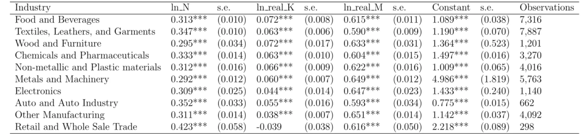
Table 1.3 shows the results of estimating the CRTS production function (Model 1) for 10 main manufacturing industries, including retail and wholesale trade, with country and year fixed-effects. The manufacturing industries have been classified according to the 2 digit ISIC code. To increase observations per group, smaller industries are merged with larger industries (for e.g., leather is merged with garments and textiles). To allow industry differences in the production parameters, I run regressions for each industry separately and include country and year fixed-effects. All of the estimated parameters are significant at a 1% level. The coefficients on intermediate inputs are mostly stable between industries and fluctuate from 0.65 for metals, machineries, and electronics to 0.59 for textiles, garments, and auto industry. Table 1.4 shows the coefficients of the production function for Model 1-3 with country

(27)

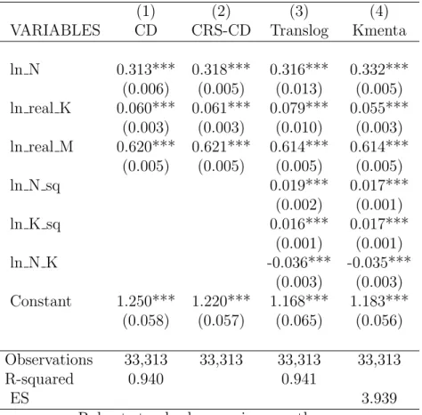
and year fixed- effects.16 _{All of the estimated parameters are significant at a 1% level and}

the estimated factor coefficients are close to the known input shares. The results confirm that the manufacturing industry is labor intensive in developing countries. For the whole sample, the output elasticity of labor (human capital) is 0.313 for CD production function and 0.318 for CRTS production function. The output elasticity of capital is 0.06 for both the CD and CRTS model. For the CD production function, a 10% increase in capital is associated with an increase of 0.6% in output. The output elasticity of intermediate inputs is 0.62 for CD and CRTS production function. This implies that, for the CD production function, an increase of 10% in intermediate inputs is associated with an increase of 6.2% in output. To sum, approximately 32% of the production output is allocated to human capital, 62% to intermediate inputs, and 6% to capital. The estimated parameters are similar in columns (3) and (4) which represent the results from estimating the Translog and Kmenta production function.

1.3.4 Identify markups

The next step is to calculate markup as µit = β_αm

it from the models estimated above. Bm

is the scalar coefficient for intermediate inputs obtained in Model 1-3 and αit is the share of expenditure for intermediate inputs in total sales. The interpretation of a high markup of firm is that the firm has high market power or faces a less market competition. It also suggests that the firm is able to charge a higher markup compared with a lower-markup firm that faces several competitors in the market. For statistical estimation of markups, I have eliminated high leverage points that is, for log markup, values below -0.39 and higher than 5 have been eliminated from the sample. In order to ensure the sample of the firms are representative of the true population, I re-estimated the sample by replacing values less than -0.39 with -0.39 and values higher than 5 with 5. The results are comparable. The mean markup is 2.03 from the 3 models and the median is around 1.27.

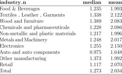
Table 1.5 shows the differences between the markup values across industries. Both the mean and the median values fall in the reasonable 1-2 range. The three industries with

(28)

higher markups are wood and furniture (1.38), textiles, garments, and leather (1.33), and electronics (1.24). Conversely, the three industries with lowest markups (at the level) are the auto and its components (0.97), non-metallic and plastic materials (1.21), and chemicals and pharmaceuticals (1.22). Note: for empirical analysis I use markup estimates from the industry-level CRTS model.

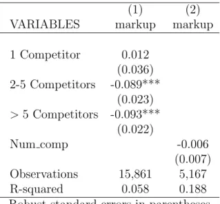
To ensure validity and robustness to the markup estimates, I regress the firm’s reported intervals for number of competitors on markup. Table 1.6 reports the results using an OLS regression with country, industry, and year fixed-effects. This regression will shed light on whether an increase in the number of competitors leads to lower markups. If the results hold, the markup estimate is consistent because higher markup indicates less competition in the market. The results confirm the hypothesis that firms facing competitors greater than two, but less than five, and greater than five see a decrease in markup. These findings are statistically significant at the 1% level.

1.3.5 Other Controls

Following previous firm-level studies, I control for various firm-level characteristics that can influence the relationship between competition and corruption. Batra et al. (2003) find that private firms are more likely to bribe, pay a higher revenue share as bribes, and more likely to consider bribe as an obstacle. Similarly, firms with large private, foreign, or government shares could face different bribe environments in dealing with public officials. Hence, I include a dummy variable equal to one for firms with more than 50% of percentage of ownership by private domestic individuals, companies or organizations (prishare), equal to two for percentage of firm owned by private foreign domestic individuals, companies or organizations (f orshare), and zero for more than 50% ownership by government or state (govshare). In my sample, 93% of the firms have some degree ofprishare, 12% of firms with some degree of forshare and 2% of firms with some degree of govshare.

Age is calculated as the logarithmic difference between the survey year and and the year in which the establishment started its operation. The suggested direction ofage is mixed in the literature. On the one hand, young firms could pay more bribes relative to older firms to

(29)

enter the market. Alternatively, older firms could pay more bribes compared to young firms to remain in the market.

I also include a variable on export status, whereexporter is a dummy variable representing a value one if the sum of indirect exports (sold domestically to third party that exports products) and direct exports is greater than 50%, with national sales as the benchmark. Studies have shown that firms that export internationally, as compared to domestic sales, might be more prone to the government rent extraction to avoid customs or taxes. Lastly, I control for the capital city since most government offices are located in the city center.

capital is a dummy variable with a value of one for firm’s located in the capital city. All else equal, I expect a positive relation between capital and bribes which indicates the firm’s influence on local government officials.

1.4 Methodology

The literature on the effects of competition on corruption has generated concerns as the cross-country studies do not address potential omitted biases. To overcome these problems, I estimate the following probit model using firm-level controls that could determine corruption. An advantage of using the firm-level data is that it sheds light on how a firm’s operating environment, within a specific industry or country, can effect the firm’s decision to bribe government official. The probit model is estimated with maximum likelihood methods and takes the following form:

P(Bribeit = 1) =P(β1markupit+β2Xit+δc+δt+δj +it>0) (1.11)

whereBribeitrepresents dummy variables for the two corruption indicators: sale-based bribe measure (bribe sales) and contract-based bribe measure (contract sales). More specifically, the dummy variable for the sales-based bribe measure (dummy sales) represent a value of one if firmiin countrycat timetreported a positive value for bribe indicated as percentage of total sales, while the dummy variable for the contract-based (dummy contract) measure represents a value of one if firmi in country c at timet reported a positive value for bribes

(30)

indicated as percentage of contract value. The main independent variable is markup which is estimated as the ratio of output elasticity of intermediate inputs to the total share of expenditure on intermediate inputs. The model also controls for firm-level characteristics (Xit) that could determine bribe incidences. These firm-level controls include firm’s age, export status, ownership status, and capital. In addition, the equations include country, industry, and year-fixed effects (denoted as δc, δj, and δt,respectively).

Since the sample includes 95 different countries from four continents, the inclusion of country-fixed effects controls for countrywide factors- country’s legal system, legal origin, rule of law, and regulation of various economic activities that could influence corruption (Treisman (2000a)). The inclusion of industry-fixed effects is to control for the exogenous variation in firm productivity that can influence the relationship between markups and bribe payments. In the same vein, the inclusion of time fixed-effects is to capture any macroeco-nomic trend or policies of a country that could potentially influence the firm’s intention to bribe. All three models use robust standard errors clustered at the country-industry level. This is to allow errors to be correlated within the same country and industry. Equation (1.11) is also estimated using logit and linear probability model for robustness.

Given that almost 75 % of the firms report zero informal payments for the corruption indexes, the Ordinary Least Squares (OLS) results can lead to biased estimates. Therefore, I also estimate the following Tobit mode with a lower bound set to zero:

bribeit =β1markupit+β2Xit+δc+δt+δj +it (1.12)

In equation 1.12, the dependent variable represents the percentage of total annual sales or total estimated value of bribe payment (sales based bribe) and the percent of the contract value paid in informal payments to secure the contract (contract based bribe). All other right hand side variables remain the same as in equation 1.11.

(31)

1.5 Results

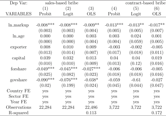
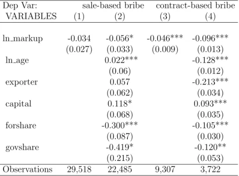
This section illustrates the econometric analysis of the relationship between firm-level markup and corruption, while controlling for firm’s age, location, ownership status, and export status. First, I estimate whether high markup firms operating in less competitive environments are less likely to engage in corruption using the probit, logit, and linear prob-ability model in table 1.7. If the firm’s competition determines the amount of bribes paid, high markup firms (less competition) should be negatively correlated with bribes. More specifically, the results of equation 1.11 are reported and include country, industry, and year fixed-effects. All of these estimations include standard errors clustered at country-industry levels. The dependent variable in columns 1-3 are a binary assigned a value of one if the firm responded with a positive value for the sales-based bribe measure, while the dependent variable in columns 4-6 is a binary with a value of one if the firm responded with a positive value for contract-based bribe measure. Columns 1 and 4 report the marginal effects of the probit model. Columns 2 and 5 report the point estimate of the logit model, while columns 3 and 6 represent the coefficient estimates of the linear probability model. As expected, the coefficients of markup are negative and statistically significant at the 5% levels in all columns. The results show that high markup firms, compared to less markup firms, are less likely to bribe as measured by both the sales-based bribe and contract-based bribe measure. Second, in table 1.8, I look at the results for the tobit model with country-industry clustered standard errors. Specifically, equation 1.12 is estimated with firm-level controls and fixed effects. The estimates in column 1 and 3 include markup as the only independent variable with country, industry, and year fixed-effects. Columns 2 and 4 add other firm-level controls. The dependent variable in columns 1-2 is bribes measured as percentages of total sales (bribe sales) and the dependent variable in column 3-4 is bribe measured as percentages of contract value. These variables are in logged terms. The results show that high markup firms decrease the incidence of bribes paid. For the sales-based bribe measure, a 10% increase in markup decreases the incidence to bribe by 0.5 percent, which is statistically significant at the 1% level. In other words, the elasticity of the sales-based bribe measure with respect to markup is -0.05. The results are similar for the contract-based bribe measure in columns

(32)

3-4. A 10% increase in markup decreases the incidence to bribe for the contract-based bribe measure by 0.9 percent. The result is statistically significant at 1 % level. As Beck and Maher (1986) explain, the model for contract-bribes can be compared to a competitive bidding model where the expected rent increases with the number of bidders. The results from the contract-based bribe measure, therefore, suggest that firms with high market power might (less bidders) likely already have established networks and are less likely to engage in bribes to get things done.

Next, I look at the firm-level characteristics in each model where several features are worth noting. Age enters the equation positively which supports the hypothesis that older firms, compared to younger firms, are more likely to bribe. Capital is positive and significant suggesting firm’s operating in the capital city are more likely to bribe. The positive sign may be due to most government offices also being located in capital cities. Likewise, the firm’s export status (=1 if exporter) enters the equation positively implying exporters are more likely to engage in bribes. Ownership variables are negative and significant. Compared to firms with private firm owners, foreign and government owners are less likely to bribe.

These results as consistent with previous literature in which stronger (weaker) market competition is associated with higher (lower) bribes. However, it should be noted that the markup results are different from the previous two studies. In this paper, markup is calcu-lated as the ratio of output elasticity of intermediate inputs to the revenue share of interme-diate inputs. Both previous papers are unable to find a statistically significant relationship between markup and bribes, although the signs are correct. Thus, the results suggest that the relationship between competition at the firm-level is economically meaningful and highly robust to various firm-level controls on corruption.

Finally, I provide a series of checks by replacing markup with other competition measures to see if the results continue to hold. The first measure is an indicator on whether the firm faces informal competition in the market. The WBES specifically asks “Does the firm face informal competition against informal or unregistered firms?” Based on responses to this question, a binary variable(informal comp)is created where responses “yes” are coded as one and zero otherwise. The level of competition a firm faces, based on whether there is informal competition in the market, is difficult to interpret as the exact number of competitors are

(33)

unknown. However, as La Porta and Shleifer (2014) show that informal firms can account to about 50 % of economic activity in developing countries, including this measure is important. The second measure is the logarithm of one plus the number of competitors reported by the firm (Num Comp). This is different from the interval range listed below because it asks the firm to provide a value for the exact number of competitors. This measure, however, has its concerns. A large firm potentially could have several small size firms as competitors which might not impact a large firm’s operation. On the other hand, a large firm could potentially have several large size firms as competitors which might have a big impact on a large firm’s operation. In addition, the sample size is relatively small (about 7,000 observations) for this measure and including country, industry, and year fixed effects could lead to a loss of degrees of freedom. The third measure is range of number of competitors that denotes the intensity for competition. More specifically, the survey question asks “for the main market in which this establishment sold its main product, how many competitors did this establishment’s main product/product line face?” The survey only provides four categories for a response and the data is coded as follows: no competition (coded 0, used as the benchmark); competitor=1 (coded 1); competitors between 2-5 (coded 2); Competitors >5 (coded 3).

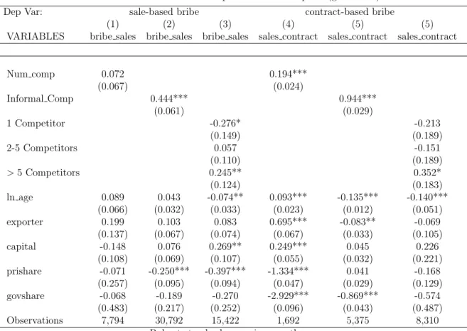
Table 1.9 reports the results of estimating a series of different measures of competition on corruption with the tobit model 1.12. Overall, the estimated result confirms that greater market competition increases the incidence to bribes. The dependent variable in columns 1-3 is the sales-based bribe measure and the dependent variable in columns 4-6 is the contract-based bribe measure. In column 1, the number of competitors is insignificant but has the correct sign. This could be due to less observations and the loss of degrees of freedom due to inclusion of fixed effects. Column 2 indicates that firms facing no informal competitors are less likely to bribe. The sales-based bribe measure increases by 0.44 units for firms facing informal competition, which is statistically significance at the 1% level. For the interval of competitors, firms facing one competitor (compared to none) are less likely to bribe. In other words, firms facing competition (with one firm) decreases the incidence of bribes for sales-based bribe measure by 0.276 units. This relationship is statistically significant at the 10% level. Similarly, firms that face competition with more than 5 firms (compared to

(34)

none), the incidence to bribes, measured by the sales-based bribe indicator, increases by 0.245 units. This result is statistically significant at the 5% level. For the contract-based measure in column 4, the coefficient on the number of competitors is significant at the 1 % level. In column 5, the coefficient of informal competition is positive and significant at the 1% level. The results indicate that there is about a 0.94 units increase in contract-based bribe measure for firms facing informal competition. The last column includes the intervals of number of competitors. Firms facing 5 or more competitors are more likely to engage in bribes as measured by the contract-based bribe measure.

Two points are noteworthy. First, the results presented in this paper are consistent with previous research that have utilized firm-level data to analyze the competition-corruption link. Despite differences in our data sample and measurement of market competition, this paper arrives at the same conclusion that higher (lower) market competition levels increases (decreases) the incidence to bribe. Second, the results are consistent across alternative measures of market competition when firm-level controls are employed in the models.

1.6 Conclusion and Limitations

This paper revisits the link between market competition and corruption using the WBES data for 95 developing countries from 2006-2016. For my analysis, I examine market compe-tition as firm-level markup which is calculated as the ratio of output elasticity of intermediate inputs to expenditure share of intermediate inputs. Previous empirical research at the firm-level have calculated markup as the profit-sales ratio; however, this method might not be accurate because the firms are less likely to maximize profits and more likely to hire excess labor in developing countries. In addition, these studies do not find a statistically signif-icant relationship between markup and corruption. This paper, therefore, contributes to the literature by finding a statistically significant negative correlation between markup and corruption. This result is consistent across other measures of competition including number of competitors and informal competition. Thus, I conclude that firm-level competition does indeed matter in determining the levels of corruption.

(35)

endogeneity associated in production function estimation is ignored. However, given the lack of dynamic panel data, the best alternative method to generate the input coefficients is with the inclusion of country, industry, and year fixed-effects. Another downside is the significant reduction in observations due to focus on the manufacturing sector. The future version of the paper will explore the service sector and find an appropriate instrument to test the exogenous variation in markup.

My findings have implications for designing policies related to fair competition in de-veloping countries. It should be noted that this paper does not recommend a decrease in market competition to decrease the level of corruption. But, it is of importance to figure out the extent to which a firm has market power and if there are any costs associated with the high market power. If the costs associated with the monopoly power are greater than the costs associated bribery, then it might be important to look deeper at any policies that lead to fairer competition. In addition, it is important to explore the extent to which firms cluster together for the positive relationship between competition and corruption to hold. Do the competitors have to be located in the same city or region? How much of monopoly power does the firm possess in a specific city or region? I hope to address these questions in future works.

(36)

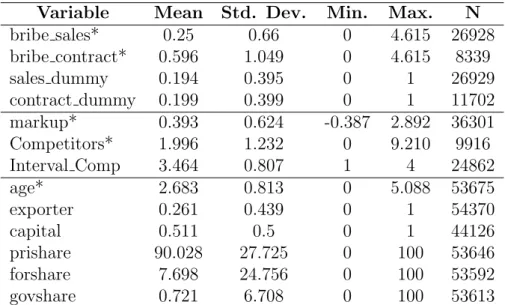
Table 1.1: Summary statistics for main variables

Variable Mean Std. Dev. Min. Max. N

bribe sales* 0.25 0.66 0 4.615 26928 bribe contract* 0.596 1.049 0 4.615 8339 sales dummy 0.194 0.395 0 1 26929 contract dummy 0.199 0.399 0 1 11702 markup* 0.393 0.624 -0.387 2.892 36301 Competitors* 1.996 1.232 0 9.210 9916 Interval Comp 3.464 0.807 1 4 24862 age* 2.683 0.813 0 5.088 53675 exporter 0.261 0.439 0 1 54370 capital 0.511 0.5 0 1 44126 prishare 90.028 27.725 0 100 53646 forshare 7.698 24.756 0 100 53592 govshare 0.721 6.708 0 100 53613

Notes: * denotes the variable is entered in log form. bribe sales is the log of one plus bribe measured as the percentage of total sales. bribe contract is the log of one plus bribe measured as per-centage of contract value. Markup is the log of ratio of the output elasticity from the production function to share of expenditure of on intermediate inputs. Competitors is logarithm of one plus the number of competitors reported by the firm. Interval comp is the intervals for number of competitors (0; Competitor=1; Com-petitors between 2-5; ComCom-petitors >5). Age is the log difference between the survey year and and the year in which the establish-ment started its operation. Exporter is a dummy variable where if indirect exports - sold domestically to third party that exports products- and direct exports > 5% is coded as one and zero oth-erwise. Capital is a dummy that takes on 1 if the firm is located in the capital city, 0 otherwise. For ownership, prishare, forshare, govshare represent the percentage of ownership by private, foreign, government parties.

(37)

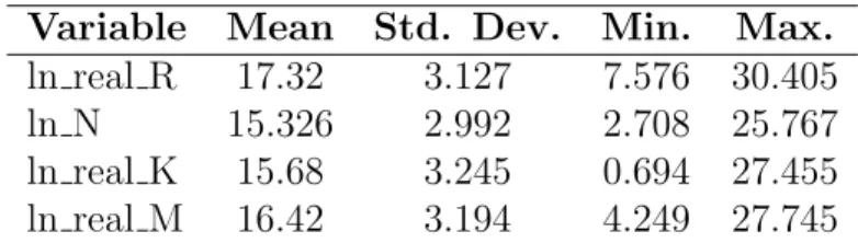
Table 1.2: Summary statistics for Production Variables

Variable Mean Std. Dev. Min. Max.

ln real R 17.32 3.127 7.576 30.405

ln N 15.326 2.992 2.708 25.767

ln real K 15.68 3.245 0.694 27.455 ln real M 16.42 3.194 4.249 27.745 Notes: All variables represent log transformation. R is total sales of the firm, K is the net book value, N is the wage bill, M is intermediate inputs. All values are in 2005 U.S. dollars.

(38)

Sharma

29

Table 1.3: Production Function Estimates By Industry with Fixed Effects

Industry ln N s.e. ln real K s.e. ln real M s.e. Constant s.e. Observations

Food and Beverages 0.313*** (0.010) 0.072*** (0.008) 0.615*** (0.011) 1.089*** (0.038) 7,316

Textiles, Leathers, and Garments 0.347*** (0.010) 0.063*** (0.006) 0.590*** (0.009) 1.190*** (0.070) 7,887

Wood and Furniture 0.295*** (0.034) 0.072*** (0.017) 0.633*** (0.031) 1.364*** (0.523) 1,201

Chemicals and Pharmaceuticals 0.333*** (0.014) 0.063*** (0.010) 0.604*** (0.015) 1.497*** (0.016) 3,270 Non-metallic and Plastic materials 0.312*** (0.016) 0.066*** (0.009) 0.622*** (0.016) 1.009*** (0.065) 4,016 Metals and Machinery 0.292*** (0.012) 0.060*** (0.007) 0.649*** (0.012) 4.986*** (1.819) 5,763

Electronics 0.309*** (0.025) 0.044*** (0.014) 0.647*** (0.023) 1.433*** (0.240) 1,140

Auto and Auto Industry 0.352*** (0.033) 0.055*** (0.016) 0.593*** (0.034) 0.775*** (0.015) 662

Other Manufacturing 0.311*** (0.014) 0.038*** (0.007) 0.651*** (0.014) 1.142*** (0.037) 4,092

Retail and Whole Sale Trade 0.423*** (0.058) -0.039 (0.038) 0.616*** (0.050) 2.218*** (0.089) 298

Notes: OLS regression for each industry is run separately with country and year fixed-effects. All variables represent log transformation ln(x+ 1).

R is total sales of the firm, K is the net book value, N is the wage bill, M is intermediate inputs. All values are in 2005 U.S. dollars.. Robust standard errors in brackets. *** p<0.01, ** p<0.05, * p<0.1

(39)

Table 1.4: Production Function Estimates with Fixed Effects

(1) (2) (3) (4)

VARIABLES CD CRS-CD Translog Kmenta

ln N 0.313*** 0.318*** 0.316*** 0.332*** (0.006) (0.005) (0.013) (0.005) ln real K 0.060*** 0.061*** 0.079*** 0.055*** (0.003) (0.003) (0.010) (0.003) ln real M 0.620*** 0.621*** 0.614*** 0.614*** (0.005) (0.005) (0.005) (0.005) ln N sq 0.019*** 0.017*** (0.002) (0.001) ln K sq 0.016*** 0.017*** (0.001) (0.001) ln N K -0.036*** -0.035*** (0.003) (0.003) Constant 1.250*** 1.220*** 1.168*** 1.183*** (0.058) (0.057) (0.065) (0.056) Observations 33,313 33,313 33,313 33,313 R-squared 0.940 0.941 ES 3.939

Robust standard errors in parentheses *** p<0.01, ** p<0.05, * p<0.1

Notes: OLS regression for each specification includes year and country fixed effects. Results are similar when industry fixed effects are used. All variables represent log transformation

ln(x+ 1). R is total sales of the firm, K is the net book value, N is the wage bill, M is intermediate inputs. All values are in 2005 U.S. dollars.. Robust standard errors in brackets. *** p<0.01, ** p<0.05, * p<0.1

(40)

Table 1.5: Level Markups by Sector

industry n median mean

Food & Beverages 1.235 1.993

Textiles , Leather , Garments 1.338 2.122

Wood and furniture 1.389 2.083

Chemicals and pharmaceuticals 1.228 2.086 Non-metallic and plastic materials 1.217 1.996

Metals and Machinery 1.248 2.017

Electronics 1.255 2.150

Auto and auto components 0.975 1.648

Other manufacturing 1.373 1.992

Retail 1.117 2.070