Gradient based sequential Markov chain Monte Carlo for multitarget tracking with correlated measurements

multitarget tracking with correlated measurements

.

White Rose Research Online URL for this paper:

http://eprints.whiterose.ac.uk/120920/

Version: Published Version

Article:

Lamberti, R., Septier, F., Salman, N. et al. (1 more author) (2018) Gradient based

sequential Markov chain Monte Carlo for multitarget tracking with correlated

measurements. IEEE Transactions on Signal and Information Processing over Networks, 4

(3). pp. 510-518. ISSN 2373-776X

https://doi.org/10.1109/TSIPN.2017.2756563

[email protected] https://eprints.whiterose.ac.uk/

Reuse

This article is distributed under the terms of the Creative Commons Attribution (CC BY) licence. This licence allows you to distribute, remix, tweak, and build upon the work, even commercially, as long as you credit the authors for the original work. More information and the full terms of the licence here:

https://creativecommons.org/licenses/

Takedown

If you consider content in White Rose Research Online to be in breach of UK law, please notify us by

Gradient-Based Sequential Markov Chain Monte

Carlo for Multitarget Tracking With

Correlated Measurements

Roland Lamberti

, Franc¸ois Septier, Naveed Salman, and Lyudmila Mihaylova

, Senior Member, IEEE

Abstract—Measurements in wireless sensor networks (WSNs) are often correlated both in space and in time. This paper focuses on tracking multiple targets in WSNs by taking into considera-tion these measurement correlaconsidera-tions. A sequential Markov Chain Monte Carlo (SMCMC) approach is proposed in which a Metropo-lis within Gibbs refinement step and a likelihood gradient proposal are introduced. This SMCMC filter is applied to case studies with cellular network received signal strength data in which the shad-owing component correlations in space and time are estimated. The efficiency of the SMCMC approach compared to particle fil-tering, as well as the gradient proposal compared to a basic prior proposal, are demonstrated through numerical simulations. The accuracy improvement with the gradient-based SMCMC is above 90%when using a low number of particles. Thanks to its sequen-tial nature, the proposed approach can be applied to various WSN applications, including traffic mobility monitoring and prediction.

Index Terms—Multiple target tracking, correlated shadowing, sequential Markov Chain Monte Carlo (SMCMC), gradient-based likelihood proposal.

I. INTRODUCTION

T

RACKING multiple mobile targets is a challenging task which has applications in a number of fields, including that of wireless cellular communication networks and mobility prediction for intelligent transportation systems. In this area, the main structure of a system will feature target nodes whose kinematic states are unknown and need to be estimated; and sensor nodes receiving some type of noisy information about the target nodes, from which an estimation of their states can be inferred.

A variety of methods have been developed in order to solve this localization problem. The more common range-based

Manuscript received September 22, 2016; revised May 2, 2017 and July 24, 2017; accepted September 5, 2017. Date of publication September 25, 2017; date of current version August 7, 2018.This work is supported by the UK Engineering and Physical Sciences Research Council (EPSRC) via the Bayesian Tracking and Reasoning over Time (BTaRoT) under Grant EP/K021516/1. The associate editor coordinating the review of this manuscript and approving it for publication was Dr. Marcelo Bruno.(Corresponding author: Roland Lamberti.)

R. Lamberti is with the IMT T´el´ecom Sudparis, Univ. Paris-Saclay, CNRS UMR 5157 - SAMOVAR, Evry 91011, France (e-mail: roland.lamberti@ telecom-sudparis.eu).

F. Septier is with the IMT Lille Douai, Univ. Lille, CNRS UMR 9189 -CRIStAL, Lille F-59000, France (e-mail: [email protected]).

N. Salman and L. Mihaylova are with the University of Sheffield, Sheffield S10 2TN, U.K. (e-mail: [email protected]; L.S.Mihaylova@sheffield. ac.uk).

Digital Object Identifier 10.1109/TSIPN.2017.2756563

methods (as opposed to range-free methods) depend on the dis-tances between nodes, through measurements of received signal strengths (RSS), signal time-of-arrivals (ToA) [1] or angle-of-arrivals (AoA) [2] originating from the targets. Both ToA and AoA approaches allow for accurate distance estimations lead-ing to good localization, however ToA requires synchronized clocks on the target nodes, while AoA requires an array of antennas and is still sensitive to errors due to multipath, mak-ing them costly solutions. The received signal strength tech-nique [3] is a much more direct and simple approach, with low implementation costs; as such, it is a recurrent subject of performance optimization attempts. Taking into account the shadowing correlation (Gudmunson’s model [4], [5]) between different nodes (targets or sensors), which capitalizes on the fact that in a given environment, closeby areas present more or less similar behaviors with regard to shadowing, and may thus be modeled as highly correlated, is one such way of im-proving this technique. A few examples of research include [6] which studies the combination of measurement correlation and shrinkage estimation of the covariance matrix for signif-icant performance improvements, but is limited to the static case. In [7]–[10] the measurement correlations are taken into account and refined particle filtering (or Sequential Importance Resampling - SIR) algorithms are implemented. This results in high localization accuracy, however these algorithms inherently suffer from the limitations of the particle filtering approach. Although this approach is known to be an effective way of solv-ing non-linear problems, it performs poorly in high-dimensional state-spaces [11].

In this paper, we present a novel Bayesian solution to tracking problems with correlated measurements based on an advanced Monte-Carlo algorithm. Firstly, we take into account the shad-owing correlations both spatially and in time, that is, between either current or past positions of any targets. This allows for performance improvements both due to the correlations in time between positions of a single target, and due to the correlations between trajectories of different targets which may cross at some point in time. Finally, in order to efficiently solve the Bayesian tracking problem, we propose to use a Sequential Markov Chain Monte Carlo (SMCMC) algorithm. This technique, which is still largely under-exploited in the signal processing literature, allows for more robust and overall better performance than the more classical particle filtering, especially in high-dimensional systems [12]–[14]. The combination of these two features thus

has a good potential for overall robustness in tracking perfor-mance in a wide range of scenarios. Preliminary results, includ-ing experimental analyses regardinclud-ing the benefits of takinclud-ing into account the spatio-temporal shadowing correlation, are already reported in our previous work [15]. We now detail and justify our choice of the SMCMC methodology and complete these results by replacing the prior proposal density of the Gibbs re-finement step with a likelihood gradient proposal. This allows to better capitalize on informative measurements and guides the particles towards high-likelihood zones, increasing the ef-ficiency of the algorithm. Finally, we present new simulation results demonstrating the benefits of this distribution over the prior and further justifying the superiority of SMCMC over SIR in our model, when both have similar sampling costs and use the same proposal densities.

The paper is structured as follows. Section II details the choice of the target and observation models. Section III-B explains the Bayesian framework used as well as the SMCMC solution, and Section IV details how to integrate the likelihood gradient in the proposal density of the Gibbs refinement step. Simulation results using synthetic data on the superiority of SMCMC with Gibbs refinement compared to SIR with resample-move, and the benefits of this gradient proposal compared to the prior, are pre-sented and analyzed in Section V, while Section VI highlights the main conclusions of this work.

II. TARGET ANDOBSERVATIONMODELS

A. Target State and Motion Models

In a 2-dimensional (2-D) network, the kinematic state of a single target at discrete time step t may be defined as a vector of positions and velocitiesxt= [xt,x, xt,y, xt,x˙, xt,y˙]T,

although it could also contain accelerations or other vari-ables of interest. Here, N∗ _{represents the set of all}

natu-ral numbers excluding 0; the kinematic state{xt,1:N}t∈N∗ =

{[(xt,1)T,(xt,2)T, . . . ,(xt,N)T]}t∈N∗ of a set ofN targets is considered to be a stochastic Markov process such that at any time step t, the transition probability density function (pdf)

p(xt,1:N|x1:t−1,1:N) =p(xt,1:N|xt−1,1:N)is known and can ei-ther be evaluated point-wise or sampled from.

B. Correlated Observation Model

Consider a set ofNtargets evolving from time 1 to timeT,

x1:T ,1:N, and a set ofM immobile sensorss= [s1,· · · ,sM] where si_{= [s}i

x, siy]T is the position of thei-th sensor fori∈

{1, . . . , M}. We suppose that both N and M are fixed and known in this model. Throughout the paper, with the exception of square functions, superscripts will be used to denote a sensor

i, a particlenor a Monte Carlo runl(in the simulations section), and subscripts will mostly be used to denote a time stept, a target

jor a component{x, y,x,˙ y˙}. At timet∈ {1,· · · , T}, a target

j∈ {1,· · ·, N}transmitting a signal with powerPt,j causes a

sensorito receive a signal with powerPi

t,j (the data association problem is assumed to be resolved, for example it could be assumed that the targets emit during preassigned epochs). The corresponding path-loss can be expressed as

Li

t,j = 10 log10 Pt,j −10 log10 Pt,ji (1)

The observed path-loss signalyi

t,j at the sensor can empiri-cally be modeled [16]–[19] as

yt,ji =Lit,j − L0 = 10αlog10 d(xt,j,si) +wit,j (2)

where

d(xt,j,si) =

(xt,j,x−six)2+ (xt,j,y−siy)2 (3)

corresponds to the Euclidean distance between the position of thej-th target at timetand thei-th sensor.L0is the path-loss

sig-nal at a reference distance of usually 1 meter away from the sen-sor;αis the path-loss exponent (PLE) assumed known (or accu-rately estimated in a real application); andwi

t,j ∼ N(0,(σt,ji )2) is the realization of a random variable modeling the log-normal shadowing effect, with σt,ji the shadowing standard deviation associated with the link between the i-th sensor and the j-th target. Thus, the shadowing effect introduces a multiplicative factor in terms of distance which means the corresponding er-ror induced is proportional to the distance itself. Therefore, this error will remain significant should the distance increase con-siderably. The standard deviationσi

t,j is assumed to be constant over time, and we also consider the region of surveillance to be limited enough not to challenge the sensivity of the sensors.

In order to account for the spatio-temporal shadowing correla-tions between two posicorrela-tions within the network, we use the Gud-munson model [4]. Thus the correlation between thej-th target at timerand thek-th target at timet, for(j, k)∈ {1, . . . , N} and(r, t)∈ {1, . . . , T}, is

Corr(xr,j,xt,k) = exp

−d(xr,j,xt,k)

Dc

(4)

whereDcis the decorrelation distance used in the Gudmundson model, which depends on the environment (field measurements in [20] suggest values forDcfor different environments) and is assumed to be known or previously estimated.

By defining:

– fi_(x

t,j) = 10αlog10(d(xt,j,si))the exact path-loss sig-nal between the position ofxt,j and that ofsi;

– ρi_(x

r,1:N,xt,1:N) a N×N matrix whose (j, k) term [ρi_(x

r,1:N, xt,1:N)]j,k =σir,jσt,ki exp

−d(xr , j,xt , k) Dc

represents the covariance between the measurements at theith_{sensor corresponding tox}

r,j andxt,k;

the collection of all the path-loss measurements observed at thei-th sensor until timetis then distributed according to the following multivariate Gaussian densityp(yi

1:t,1:N|x1:t,1:N):

yi_1:t,1:N =

⎡ ⎢ ⎢ ⎢ ⎢ ⎢ ⎢ ⎢ ⎢ ⎢ ⎢ ⎢ ⎢ ⎢ ⎢ ⎣ yi

1,1

.. . yi 1,N .. . yi t,1 .. . yi t,N ⎤ ⎥ ⎥ ⎥ ⎥ ⎥ ⎥ ⎥ ⎥ ⎥ ⎥ ⎥ ⎥ ⎥ ⎥ ⎦ ∼ N ⎛ ⎜ ⎜ ⎜ ⎜ ⎜ ⎜ ⎜ ⎜ ⎜ ⎜ ⎜ ⎜ ⎜ ⎜ ⎝ ⎡ ⎢ ⎢ ⎢ ⎢ ⎢ ⎢ ⎢ ⎢ ⎢ ⎢ ⎢ ⎢ ⎢ ⎢ ⎣

fi_(x

1,1)

.. .

fi_(x

1,N) .. .

fi_(x t,1)

.. .

fi_(x t,N) ⎤ ⎥ ⎥ ⎥ ⎥ ⎥ ⎥ ⎥ ⎥ ⎥ ⎥ ⎥ ⎥ ⎥ ⎥ ⎦

with Ri

t the (N×t, N×t) observation covariance matrix which includes correlations in the measurements due to the close proximity of target positions, both “spatially” at a given time step and “spatio-temporally” between positions of different targets from different time steps, and can be expressed in blocks as:

Ri_t=

⎡

⎢ ⎢ ⎢ ⎣

ρi_(x

1,1:N,x1,1:N) · · · ρi(x1,1:N,xt,1:N)

..

. . .. ...

ρi_(x

t,1:N,x1,1:N) · · · ρi(xt,1:N,xt,1:N)

⎤

⎥ ⎥ ⎥ ⎦

. (6)

Finally, measurements at each sensor are supposed to be inde-pendent from measurements at all other sensors - this is justified by considering scenarios where the sensor positions are immo-bile and sufficiently far apart from each other thus inducing little to no correlation. Thus the joint pdf of the measurements from several sensors can be calculated as the product of the pdfs of the measurements from each one of these sensors:

p(y1:M

1:t,1:N|x1:t,1:N) = M

i= 1 p(yi

1:t,1:N|x1:t,1:N). (7)

III. PROPOSEDBAYESIANSOLUTION

A. Recursive Inference

The aim of the Bayesian inference is to recursively estimate the states of the sequence of targets by computing the expecta-tion of its joint posterior density. At timet, this posterior density can be deduced recursively as a function of its expression from the previous time stept−1:

p(x1:t,1:N|y1:1:t,M1:N)∝

M

i= 1

p(yi_t,1:N|yi_1:t−1,1:N,x1:t,1:N)p(xt,1:N|xt−1,1:N)

×p(x1:t−1,1:N|y1:1:Mt−1,1:N). (8)

However, this density is intractable mainly due to the nonlinear relationship of the hidden states in the observations and there-fore needs to be approximated. In this posterior distribution of interest, the likelihood is obtained from (5) using classical conditional properties of the multivariate Gaussian distribution:

p(y_t,i_1:N|y_1:i_t−1,1:N,x1:t,1:N) =Nµi_t,Σi_t, (9)

where

µ_ti=µ₂+Σ2,1Σ1−,11(z−µ1),

Σi_t =Σ2,2−Σ2,1Σ−1,11Σ1,2, (10)

with

z=yi

1:t−1,1:N,

µ₁ = [fi(x1,1),· · · , fi(x1,N),· · ·, fi(xt−1,1),· · ·,

fi(xt−1,N)]T,

µ2 = [fi(xt,1),· · ·, fi(xt,N)]T,

Σ1,1 =Rit−1,

Σ2,1 = [ρi(xt,1:N,x1,1:N),· · · , ρi(xt,1:N,xt−1,1:N)],

Σ1,2 = [ρi(x1,1:N,xt,1:N),· · · , ρi(xt−1,1:N,xt,1:N)]T,

Σ2,2 =ρi(xt,1:N,xt,1:N). (11)

Given that any measurement is dependent on all of the other measurements at any time step, the sizes of the mean vector and covariance matrix of the observation defined in (5) grow with time. As a consequence, the cost of the computation of the likelihood in (9) that will be required in the filtering algorithm increases with time. In this paper, we therefore propose to use a strategy in order to have a constant computational cost by using a restriction of the size of the used history of positions, for instance through a sliding time window. One drawback of such an approximation is that it could imply the loss of interesting correlation information in cases where some targets approach past trajectories of some other targets (or themselves). Indeed, although the most significant correlations may often intuitively be the ones between positions of a same target at close time steps, simply due to their inherent proximity compared to the proximity of positions from different targets, this still depends on the chosen target motion model. It is likely to be the case if the targets move completely independently, which is clearly not always a correct assumption in real scenarios. However, the sliding time window approximation may also help in avoiding possible numerical problems in the evaluation of the likelihood (due to the inversion of a large covariance matrix). By defining the size of this sliding time window astwindow, the computation of the likelihood in (9) will involve a modified covariance matrix of size(N×(twindow+ 1), N×(twindow+ 1))since∀(j, k)∈

{1, . . . , N}, we will considerCorr(xr,j,xt,k) = 0if|r−t|>

twindow.

In a single target scenario, the authors in [10] propose to use a sequential Monte-Carlo method, known as particle fil-ter, in order to infer the single target characteristics given the observations. However, this method suffers from intrinsic limi-tations in high-dimensional systems ([11], [21]), as the number of samples needs to increase exponentially with the variance of the weights (which is typically a linear function of the state dimension) so as to ensure that not only a single weight will be non-null. In order to obtain a more efficient algorithm for multiple target tracking, we thus propose an alternative solution based on a more advanced methodology known as Sequential Markov Chain Monte Carlo (SMCMC) [12].

B. The Proposed SMCMC Algorithm

no theoretical proofs of this yet, SMCMC has experimentally proven to be much more efficient than particle filtering (includ-ing particle filter(includ-ing augmented with MCMC resample-moves [22]) at handling high-dimensional settings, because of the se-quential nature of the algorithm allowing local exploration of the state-space with a single Markov chain at a given time step, thus reaching more relevant regions of the state-space in terms of posterior. On the contrary, a particle filter augmented with MCMC resample-moves will still suffer from the limitations of the importance sampling and resampling steps (which SMCMC omits entirely), and attempt to remedy them by constructing several independent Markov chains which is much less efficient than the SMCMC approach.

More specifically, the sequential MCMC (SMCMC) is a pow-erful sequential methodology for filtering that targets the joint posterior distribution defined in our case by (8). At a given time step, we use a MCMC procedure to make inference from this complex distribution (which is fixed for this time step). How-ever, since we do not have a closed form representation of the posterior distributionp(x1:t−1,1:N|y1:1:Mt−1,1:N)at timet−1, it will be approximated by an empirical distribution based on the current particle set:

p(x1:t−1,1:N|y1:1:Mt−1,1:N)≈ 1

Np Np

j= 1 δ_x(j)

1 :t−1,1 :N(

x1:t−1,1:N) (12)

whereNp is the number of particles and(j)the particle index. Then, by plugging this particle approximation into (8), we obtain

π(x1:t,1:N)∝

1

Np Np

j= 1 M

i= 1

p(yi_t,1:N|yi_1:t−1,1:N,x(_1:j_t−) _1,1:N,xt,1:N)

×p(xt,1:N|x_t−(j)_1,1:N)δ_x(j) 1 :t−1,1 :N(

x1:t−1,1:N) (13)

whereπ(x1:t,1:N), an empirical approximation of the true pos-teriorp(x1:t,1:N|y1:1:Mt,1:N)based on the particle setx

(1:Np) 1:t−1,1:N, is the target distribution of the Markov chain at time stept. At a given iterationnof the Markov chain, the variablesx1:t−1,1:N are to be drawn according to a uniform discrete distribution (selected uniformly from the setx(1:Np)

1:t−1,1:N) whereasxt,1:N is then drawn from a continuous distribution conditional to this previous sample, hence the designation “Joint Draw” for this procedure.

Then, having made many joint draws from (13) using an appropriate MCMC scheme, the converged MCMC output for variablex1:t,1:N can be extracted to give an updated particle approximation ofp(x1:t,1:N|y1:1:Mt,1:N)to be used at the next time iteration. More specifically, after a burn-in period ofNbu r n, keep every MCMC outputx(_1:j_N) =xn

1:N as the new particle set for the posterior distribution (the notation(j)is meant to include only theNp particles that are considered to be after the burn-in period, whilenmay refer to any particle of the chain). In this way, sequential inference can be achieved.

In addition to this procedure, we choose to perform an ad-ditional refinement step in order to improve the quality of the

samples corresponding to timet. Several block sampling struc-tures could be considered [23], but in this paper, we opt to sample successively each of the individual targets using a series of Metropolis-within Gibbs steps, which consists in drawing new samples component-wise, that is in our application, target-wise, conditionally to all other targets, and choosing whether to accept them. This allows to carefully move each component of our particles towards more interesting regions of the state-space, using densities that are focused on each component as opposed to the joint density used in the previous step. It should be empha-sized that our block sampling Gibbs step is in fact target-wise and thus multivariate, rather than univariate coordinate-wise. This is much more efficient since in our setting there is a strong correlation between coordinates of a single target, which means sampling a single coordinate conditionally to other coordinates of the same target would be degenerated (close to deterministic). To further take advantage of this approach, we also use a Langevin-type gradient proposal density for sampling in the refinement (this aspect will be detailed in Section IV). It is in-teresting to note that performing both a MH Joint Draw and next a component-wise Gibbs refinement is complementary. Indeed, the Gibbs step improves upon the previous joint sampling. How-ever, if we were to omit the initial Joint Draw and only perform this refinement step, the sampling might become degenerated if there is high correlation between targets’ measurements since we use a density conditional on all targets other than the current component [12]. Additionally, while in our chosen algorithm we only perform a single MH Joint Draw step, several iterations could potentially help improve the mixing for the Markov Chain [24] (once again especially when there is strong correlation be-tween blocks, which in our case would correspond to targets in close proximity).

In short, at timetand at then-th MCMC iteration, the fol-lowing procedure is thus performed to obtain samples from

p(x1:t,1:N|y1:1:t,M1:N):

r

_{Make a joint draw for}x

1:t,1:N using a Metropolis-Hastings step,

r

_{Refine the hidden state at current time}t_,x

t,1:N, using a series of Metropolis-Hastings-within-Gibbs steps. The complete proposed algorithm is summarized in Algo-rithm 1 (which also includes the Langevin-type gradient pro-posal explained in Section IV).

Following the acquisition of this set of particles (selected after a burn-in period) asymptotically drawn according to the density

p(x1:t,1:N|y1:1:t,M1:N), the target state estimation at timetcan be performed using the minimum mean square error criterion as the mean of the particles, which corresponds to the empirical approximation of the expectation of the marginalized posterior densityp(xt,1:N|y1:1:Mt,1:N):

ˆ

xt,1:N =

xt,1:Np(xt,1:N|y1:1:Mt,1:N)dxt,1:N

≈ 1

Np Np

j= 1

Algorithm 1:Proposed SMCMC for Multi-Target Tracking. At timet, to compute then-th SMCMC particle trajectory

xn

1:t,1:N: Data:y1:M

1:t,1:N (all of the measurements available at timet),

x(1:Np)

1:t−1,1:N (the particle set constituting the empirical approximation of the posterior density from timet−1),

xn−1

1:t,1:N (the result of the previous stepn−1of the algorithm)

Joint Draw using Metropolis-Hastings

– Randomly select a joint particle trajectoryx˜1:t−1,1:N by sampling it from the empirical measure of

p(x1:t−1,1:N|y1:1:t−M1,1:N)obtained at the previous time iteration:

˜

x1:t−1,1:N ∼ 1

Np Np

j= 1 δ_x(j)

1 :t−1,1 :N(

x1:t−1,1:N) (15)

– Draw a random sample for the currentt-th time step:

˜

xt,1:N ∼p(·|x˜t−1,1:N) (16)

– Calculate the acceptance ratio which compares the likelihood given˜x1:t,1:N with the likelihood givenxn1:−t,11:N (which is the one from the previous iterationn−1):

α= min

1, M

i= 1p(yit,1:N|yi1:t−1,1:N,x˜1:t,1:N)

M

i= 1p(yit,1:N|yi1:t−1,1:N,xn−

1 1:t,1:N)

(17)

– Accept this proposed particle or reject it: drawa∼ U[0,1]

if(a < α)then

accept the particle, thusxn

1:t,1:N := ˜x1:t,1:N else

reject the particle, thusxn

1:t,1:N :=xn1:−t,11:N end

Refinement using Metropolis-within-Gibbs – Successively sample each target:

forb= 1toN do

– Definex˜1:t,1:N :=xn1:t,1:N

– Draw a new sample from the gradient-based proposal densityqin (19), for theb-th target at current timet:

˜

xt,b∼q(·|xnt,b) (18)

– Calculate the acceptance ratio asα= min (1, β) whereβis from (28), with the modified particle ˜

x1:t,1:N.

– Accept this proposal particle or reject it: drawa∼ U[0,1]

if(a < α)then

accept the particle,xn t,b= ˜xt,b else

reject the particle, do not update theb-th block inxn

t,1:N end

end

Output:Samplexn

1:t,1:N

IV. GRADIENT-BASEDPROPOSALDENSITY

The choice of a relevant proposal density to propagate the kinematic states in the Metropolis-within-Gibbs refinement steps is crucial for the algorithm to be able to “lock-on” to the targets. In our case, using the prior probability density may be prone to failure especially in scenarios where this density has a large covariance matrix. Therefore, we aim to overcome this problem using a proposal density that is dependent on the observations, so as to guide the particles towards regions of the state-space which harbor high likelihood.

We choose a Langevin-type ([25], [26]) proposal densityq(·) which is based on the gradient of the target density (which includes the likelihood). For a targetk, at then-th step of the Metropolis-Hastings algorithm, the Gibbs refinement sample will be drawn as follows:

˜

xt,k∼q(·|xnt,k) =N

xn_t,k+m,Σ

(19)

where xn

t,k results from the Metropolis-Hastings Joint Draw, and

m= h

2∇(log Π(xt,k))

xt , k=xnt , k

Σ=hI4×4, (20)

hbeing a step which needs to be chosen empirically so that the performance of the algorithm is optimal, andΠ(xt,k), pro-portional to the conditional posterior density p(xt,k|y1:1:t,M1:N,

xn

1:t−1,1:N,xnt,1:N\k)for the current target of interest, being the product of the corresponding likelihood and prior terms, derived from (8); thus

Π(xt,k)

= M

i= 1

p(yi_t,1:N|yi_1:t−1,1:N,xn_1:t−1,1:N,xn_t,1:N\k,xt,k)

×p(xt,k|xnt−1,1:N,xnt,1:N\k). (21)

Using (9) and (10),

log Π(xt,k) = M

i= 1

logN

yi_t,1:N;µi_t,Σi_t (22)

+ logp(xt,k|xnt−1,1:N,xnt,1:N\k). (23)

We need to calculate the gradient of

logN

yi_t,1:N;µi_t,Σi_t

=−1

2log 2π−log|Σ i t| −

1 2

yi_t,1:N −µi_tT

×Σi_t

yi_t,1:N −µi_t (24)

with respect toxt,k and evaluate it atxnt,k. In this expression, bothµi_t andΣi_t are dependent on xt,k (see (10) and (11)). In order to simplify this problem, we assume all terms related to covariances (thusΣi

tas well as the covariance terms inµit) to be constant for the derivative. Under this assumption, denotingA=

yi

t,1:N −µit

andS= Σi

ofxt,k = [xt,k ,x, xt,k ,y, xt,k ,x˙, xt,k ,y˙]T (thusc∈ {x, y,x,˙ y˙}):

∂AT_SA

∂xt,k ,c =

∂AT_SA

∂µi t

T ∂µi

t

∂xt,k ,c

(25)

with

∂ATSA ∂µi

t

=−2SA

∂µi t

∂xt,k ,c =

0,· · · ,0,∂f

i_(x t,k)

∂xt,k ,c

,0,· · ·,0, T

(k-th component)

(26)

because all terms dependent on targets other than thek-th target have derivatives equal to 0. Moreover, the only term derived in

µi_tisµ₂(from (11)), according to our assumption, since the only

other term inµi_t that depends onxt,k is a covariance (namely

Σ2,1). On the other hand,

∂fi(xt,k)

∂xt,k

= ⎡ ⎢ ⎢ ⎢ ⎢ ⎢ ⎢ ⎢ ⎢ ⎢ ⎢ ⎢ ⎢ ⎢ ⎣

∂fi_(x t,k)

∂xt,k ,x

∂fi_(x t,k)

∂xt,k ,y

∂fi_(x t,k)

∂xt,k ,x˙

∂fi_(x t,k)

∂xt,k ,y˙ ⎤ ⎥ ⎥ ⎥ ⎥ ⎥ ⎥ ⎥ ⎥ ⎥ ⎥ ⎥ ⎥ ⎥ ⎦ = ⎡ ⎢ ⎢ ⎢ ⎢ ⎢ ⎢ ⎢ ⎢ ⎢ ⎣

10α (xt , k , x−six) (xt , k , x−six)2+(xt , k , y−siy)

2

10α

xt,k ,y−siy

(xt,k ,x−six)

2₊

xt,k ,y −siy

2 0 0 ⎤ ⎥ ⎥ ⎥ ⎥ ⎥ ⎥ ⎥ ⎥ ⎥ ⎦ (27)

the derivatives with respect to velocities being zero since the ob-servations are only dependent on the distances between targets, thus only on target positions. Thus the propagation of velocity values is handled by the prior component alone. The derivative of this prior component is calculated in a similar way, except no assumptions are necessary.

Lastly, the expression of the acceptance ratio for the refine-ment step needs to be updated as it is dependent on the proposal densityq(with the same notations as Algorithm 1):

β=

M

i= 1p(yit,1:N|yi1:t−1,1:N,x˜1:t,1:N)

M

i= 1p(yit,1:N|yi1:t−1,1:N,xn1:t,1:N)

×p(˜xt,k|x

n

t−1,1:N,xnt,1:N\k)

p(xn

t,k|xnt−1,1:N,xnt,1:N\k)

q(xn t,k|x˜t,k)

q(˜xt,k|xn_t,k)

. (28)

V. SIMULATIONRESULTS

In order to illustrate the performance improvements induced by

– using a SMCMC approach compared to a classical particle filtering approach (Section V-A with a figure showing the superiority of SMCMC the higher the dimension of the state-space is),

[image:7.594.317.534.64.242.2] [image:7.594.38.289.70.204.2]

– replacing the prior proposal density with the gradient pro-posal density (Sections V-B and V-C with figures showing

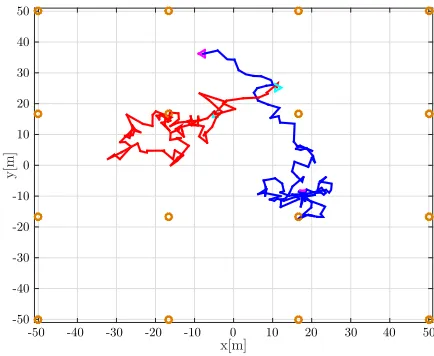
Fig. 1. Example of two chaotic trajectories withσ2

target=10 m2. The orange circles represent the sensors, the lines represent the trajectories and the_/△

symbols represent their starting/ending points, respectively.

the varying amounts of performance gains depending on shadowing noise variance and number of particles), we assume that each target evolves independently from the others in a field of 16 sensors as illustrated in Fig. 1, according to a nearly constant velocity model [27], [28] which is defined as follows for thej-th target:

xt,j =Ftxt−1,j+ut,j (29)

whereFt would be a4×4transition matrix andut,j a vector of independent realizations ofN(04,Qt)withQta4×4state noise covariance matrix, bothFtandQtdepending only on the time interval betweentandt−1. HereFtandQt are defined as:

Ft=

I2 τtI2

02 I2

,Qt =σtarget

(τ3

t/3)I2 (τt2/2)I2

(τ2

t/2)I2 τtI2

(30)

withτtthe time interval between two time steps, which is chosen constant and equal to 1 second, andσ2

target= 10m2.

Fig. 1 shows an example of two trajectories created with these parameters and chosen to be confined within a grid of sensors. Due toσ2target having a relatively large value, the trajectories

are chaotic, representing a difficult tracking scenario.

In order to assess the accuracy of the different algorithms when the measurements are randomly generated with standard deviationσ(for the shadowing noise) equal for all target-sensor links, we compute the root mean square error (RMSE) between the estimations and the real positions of the target (the estima-tions of other variables such as velocities or acceleraestima-tions are not taken into account), in time, averaged on a number of Monte Carlo (MC) runs:

RMSEt=

! ! "

1

NM CN N

j= 1

NM C

l= 1

ˆ

xl

t,j −xt,j 2 (31)

where xˆl

t,j is the estimated state of the j-th target from the

l-th MC run. Throughout this section, we chooseNM C =10,

[image:8.594.48.288.63.256.2]

Fig. 2. Log-scale performance of our SMCMC algorithm versus a SIR algo-rithm with the same Gibbs refinement step as resample-move. Low measurement noise (σ2 _{= (0.1)}2_{dB) and process noise (σ}2

target=0.01 m2).

of sensorsM = 16, a number of targetsN = 2and a number of time stepsT = 100. For reference, the experiments used Matlab software and a laptop featuring a 2.80 GHz Intel(R) Core(TM) i7-4810MQ CPU.

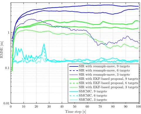
A. Performance Compared to Particle Filtering

First, we compare the proposed SMCMC algorithm with the particle filtering approach which was proposed in [10] in a sim-ilar context for single target tracking. More specifically, the particle filter used in this section is the Sequential Importance Resampling (SIR) [29] in which a resample-move strategy is em-ployed after the resampling stage in order to diversify the set of particles [22]. This strategy uses exactly the same step described as the refinement step in our proposed SMCMC, including the gradient-based proposal, thus allowing for a fair comparison between the two algorithms. For further comparison we also implement a SIR without resample-move but instead using a custom EKF-based proposal [30]. Fig. 2 shows the RMSE ob-tained with all three algorithms in whichNp = 200 particles are used to do the inference, and the actual target trajectories are generated withσ2

target =0.01 m

2_{thus much smoother than}

those from Fig. 1 (Section V-B below studies this more chal-lenging case). In this simulation, the shadowing variance is

σ2 _=(0.1)2_{dB which is a low noise in the context of our}

[image:8.594.312.551.66.247.2]

exper-iment, and different numbers of targets are used (N = 3,6,9). Indeed, the SIR algorithm’s main weakness comes from the degeneration of the importance weights in situations where ei-ther the likelihood becomes too informative (with a too small variance) and no longer covers regions where the proposal distri-bution is high, or more interestingly in difficult situations where the state-space is high-dimensional. In such a multi-dimensional scenario, the results show the significant superiority of the pro-posed SMCMC against the SIR, with computational times of the same order; additionally, the average RMSE per target remains about the same for SMCMC as the total number of targets in-creases, while it deteriorates in the case of SIR. For reference, the

Fig. 3. Log-scale performance of the SMCMC algorithm using the gradient-based proposal density versus the prior density, for high measurement noise values on the chaotic trajectory set from Fig. 1 (difficult scenario).

computational time of this experiment with 3 targets, averaged over the MC runs and the time steps, is approximately 3.4144 seconds for SIR with resample-move, 1.6141 seconds for SIR with EKF-based proposal and 3.8601 seconds for SMCMC. The difference between SIR with resample-move and SMCMC corresponds almost exactly to an increase of10%in the com-putational time, while the SMCMC method uses an additional burn-in period of precisely10% of the total number of parti-cles (in this case, 222 partiparti-cles including the burn-in, compared to 200 for SIR with resample-move and for SMCMC without burn-in). Thus, SIR with resample-move and SMCMC have a similar computational time for a single particle (and the same remarks still apply with higher numbers of targets).

B. Performance in Difficult, Noisy Scenarios

We now demonstrate the benefits of using the gradient pro-posal distribution presented in Section IV instead of the basic prior proposal in our Gibbs refinement moves, in difficult sce-narios. Given the chaotic hidden state trajectories from Fig. 1 (thusN = 2), and eitherσ2= 12dB (average-to-high measure-ment noise) orσ2_{= 4}2 _{dB (high measurement noise), we run}

our algorithm with either the prior proposal density or the gradi-ent proposal density from Section IV. Fig. 3 shows the resulting RMSE performance with respect to the time step, forNp = 500. As expected, the estimator using the gradient proposal performs better. For reference, the computational time of this experiment, averaged over the MC runs and the time steps, is approximately 1.5205 second with the prior proposal and 3.2878 seconds with the gradient proposal, when σ2_{= 1}2 _{dB. When σ}2 _{= 4}2 _dB,

the computational times are 1.8128 second and 3.8967 seconds, respectively.

TABLE I

ACCEPTANCERATIOS IN THEGIBBSREFINEMENTSTEPWHENUSINGEITHER THEPRIORPROPOSALDENSITY OR THEGRADIENT-BASEDONE, WITH

VARYINGMEASUREMENTNOISE

Prior Gradient

σ2 _{= (0.1)}2 _{0.0066 0.0392}

σ2 _{= (0.3)}2 _{0.0075 0.2669}

σ2 _{= (1)}2 _{0.0377 0.8198}

σ2 = (2)2 0.1940 0.9117

σ2 _{= (4)}2 _{0.4860 0.9500}

Fig. 4. Log-scale performance of the algorithm using the gradient-based pro-posal density versus the prior density, with low measurement noise (σ2 ₌

(0.1)2dB) and average process noise (σtarget2 =1m2).

propagated is able to reach regions of the state-space featuring much higher likelihood than with the prior proposal. Moreover, from a theoretical point of view, the gain of performance due to using the gradient proposal should decrease when the measure-ment noise increases, since this density aims to guide the sam-pled particles towards these regions of high likelihood, because then such regions become very wide and inaccurate. Table I con-firms that the gain in acceptance ratio indeed decreases when the measurement noise increases. Fig. 4 from Section V-C also confirms this by showing much larger performance gain with lower noise (and also less chaotic trajectories) than in Fig. 3’s difficult scenario.

C. Performance in Easier Scenarios With Varying Number of Particles

Another benefit of using this gradient-based density can be demonstrated when reducing the number of particles used for the filter. Indeed, using the Gaussian prior density implies that in order to draw only a few particles which will be located in regions of interest where the likelihood function is high, it is required to draw a very large number of particles in total, whereas the gradient-based density has no such drawback (as the acceptance ratios from Table I also demonstrate). Fig. 4 shows RMSE values in time for different numbers of particles, displaying how the linear gap of performance between the two

proposal densities increases when the number of particles used decreases. For reference, the computational time of this experi-ment, averaged over the MC runs and the time steps, is approx-imately 0.24 second when using 25 particles and 1.66 second when using 200 particles.

VI. CONCLUSIONS

This paper proposes a sequential MCMC solution to multi-target tracking with RSS measurements, taking into ac-count spatio-temporal correlations between targets and using a gradient-based proposal density for drawing particles in the Gibbs refinement moves. The simulation results show a perfor-mance improvement (about50% increase in accuracy) in any scenario compared to using the prior density as a proposal, and the gain is especially large (above90%) when using low number of particles or when the model considered features informative measurements. The SMCMC approach is also shown to be su-perior to particle filtering in this setting when both use the same Gibbs refinement moves.

REFERENCES

[1] I. Guvenc and C.-C. Chong, “A survey on TOA based wireless localization and NLOS mitigation techniques,”IEEE Commun.. Surveys Tut., vol. 11, no. 3, pp. 107–124, Jul.–Sep. 2009.

[2] B. Van Veen and K. Buckley, “Beamforming: A versatile approach to spatial filtering,”IEEE Acoust., Speech, Signal Process. Mag., vol. 5, no. 2, pp. 4–24, Apr. 1988.

[3] N. Patwari, A. Hero, M. Perkins, N. Correal, and R. O’Dea, “Relative loca-tion estimaloca-tion in wireless sensor networks,”IEEE Trans. Signal Process., vol. 51, no. 8, pp. 2137–2148, Aug. 2003.

[4] M. Gudmundson, “Correlation model for shadow fading in mobile radio systems,”Electron. Lett., vol. 27, no. 23, pp. 2145–2146, Nov. 1991. [5] P. Agrawal and N. Patwari, “Correlated link shadow fading in

multi-hop wireless networks,”IEEE Trans. Wireless Commun., vol. 8, no. 8, pp. 4024–4036, Aug. 2009.

[6] N. Salman, L. Mihaylova, and A. Kemp, “Localization of multiple nodes based on correlated measurements and shrinkage estimation,” inProc. Sensor Data Fusion: Trends, Solutions, Appl., Oct. 2014, pp. 1–6. [7] L. Mihaylova, D. Angelova, D. Bull, and N. Canagarajah, “Localization

of mobile nodes in wireless networks with correlated in time measurement noise,”IEEE Trans. Mobile Comput., vol. 10, no. 1, pp. 44–53, Jan. 2011. [8] L. Mihaylova, D. Angelova, S. Honary, D. Bull, C. Canagarajah, and B. Ristic, “Mobility tracking in cellular networks using particle filtering,”

IEEE Trans. Wireless Commun., vol. 6, no. 10, pp. 3589–3599, Oct. 2007. [9] B. Ferris, D. H¨ahnel, and D. Fox, “Gaussian processes for signal

strength-based location estimation,” inProc. Robot., Sci. Syst., 2006, pp. 1–8. [10] H. Noureddine, N. Gresset, D. Castelain, and R. Pyndiah, “Auto-regressive

modeling of the shadowing for RSS mobile tracking,” inProc. IEEE Int. Conf. Commun., Jun. 2011, pp. 1–5.

[11] C. Snyder, T. Bengtsson, P. Bickel, and J. Anderson, “Obstacles to high-dimensional particle filtering,”Monthly Weather Rev., Special Collection, Math. Advances Data Assimilation, vol. 136, no. 12, pp. 4629–4640, 2008. [12] F. Septier, S. K. Pang, A. Carmi, and S. Godsill, “On MCMC-based particle methods for bayesian filtering: Application to multitarget tracking,” in

Proc. 3rd IEEE Int. Workshop Comput. Advances Multi-Sensor Adaptive Process, Dec. 2009, pp. 360–363.

[13] A. Brockwell, P. Del Moral, and A. Doucet, “Sequentially inter-acting Markov chain Monte Carlo methods,” Ann. Statist., vol. 38, no. 6, pp. 3387–3411, Dec. 2010. [Online]. Available: http://dx.doi.org/ 10.1214/09-AOS747

[15] R. Lamberti, F. Septier, N. Salman, and L. Mihaylova, “Sequential Markov Chain Monte Carlo for multi-target tracking with correlated RSS mea-surements,” inProc. IEEE 10th Int. Conf, Intell. Sensors, Sensor Netw Inf. Process., Apr. 2015, pp. 1–6.

[16] K. Pahlavan and A. H. Levesque,Wireless Information Networks. New York, NY, USA: Wiley, 1995, vol. 95.

[17] T. Rappaport,Wireless Communications: Principles and Practice (Electri-cal Engineering). Englewood Cliffs, NJ, USA: Prentice-Hall, 1996. [On-line]. Available: https://books.google.fr/books?id=C_pSAAAAMAAJ [18] I. Nevat, G. W. Peters, K. Avnit, F. Septier, and L. Clavier, “Location

of things: Geospatial tagging for IoT using time-of-arrival,”IEEE Trans. Signal Inf. Process. over Netw., vol. 2, no. 2, pp. 174–185, Jun. 2016. [19] N. Patwari, J. N. Ash, S. Kyperountas, A. O. Hero, R. L. Moses, and

N. S. Correal, “Locating the nodes: Cooperative localization in wireless sensor networks,”IEEE Signal Process. Mag., vol. 22, no. 4, pp. 54–69, Jul. 2005.

[20] D. S. Baum, J. Hansen, and J. Salo, “An interim channel model for beyond-3G systems: Extending the beyond-3GPP spatial channel model (SCM),” inProc. 61st IEEE Veh. Technol. Conf., vol. 5, May 2005, vol. 5, pp. 3132–3136. [21] C. Snyder, “Particle filters, the optimal proposal and high-dimensional

sys-tems,” inProc. Seminar Data Assimilation Atmosphere Ocean. Shinfield Park, Reading, MA, USA: ECMWF, 2012, pp. 161–170.

[22] W. R. Gilks and C. Berzuini, “Following a moving target-Monte Carlo inference for dynamic Bayesian models,”J. Roy.l Statist. Soc. B (Statist. Methodology), vol. 63, pp. 127–146, 2001.

[23] G. O. Roberts and S. K. Sahu, “Updating schemes, correlation structure, blocking and parameterization for the Gibbs sampler,”J. Roy. Statist. Soc. B (Statist. Methodology), vol. 59, no. 2, pp. 291–317, 1997. [Online]. Available: http://dx.doi.org/10.1111/1467–9868.00070

[24] L. Martino, V. Elvira, and G. Camps-Valls, “The recycling gibbs sampler for efficient learning,” arXiv:1611.07056, 2016.

[25] F. Septier and G. W. Peters, “Langevin and Hamiltonian based sequential MCMC for efficient Bayesian filtering in high-dimensional spaces,”IEEE J. Sel. Topics Signal Process., vol. 10, no. 2, pp. 312–327, Mar. 2016. [26] M. Girolami and B. Calderhead, “Riemann manifold Langevin and

Hamiltonian Monte Carlo methods,” J. Roy. Statist. Soc. B (Statist. Methodology), vol. 73, no. 2, pp. 123–214, 2011. [Online]. Available: http://dx.doi.org/10.1111/j.1467–9868.2010.00765.x

[27] X. Li and V. Jilkov, “Survey of maneuvering target tracking. Part I. Dynamic models,”IEEE Trans. Aerosp. Electron. Syst., vol. 39, no. 4, pp. 1333–1364, Oct. 2003.

[28] W. Blair, “Design of nearly constant velocity track filters for tracking maneuvering targets,” inProc. 11th Int. Conf. Inf. Fusion, Jun. 2008, pp. 1–7.

[29] A. Doucet, N. De Freitas, and N. Gordon, Eds.,Sequential Monte Carlo Methods in Practice. Berlin, Germany: Springer-Verlag, 2001.

[30] A. Doucet, S. Godsill, and C. Andrieu, “On sequential Monte Carlo sampling methods for Bayesian filtering,” Statist. Comput., vol. 10, no. 3, pp. 197–208, Jul. 2000. [Online]. Available: http://dx.doi.org/ 10.1023/A:1008935410038

Roland Lamberti received the M.Sc. degree in telecom engineering from Telecom SudParis, Evry, France, in 2015. He is currently working toward the Ph.D. degree in the Department of Communications, Images and Information Processing, Telecom Sud-Paris, on the subject of high-dimensional Bayesian inference.

Franc¸ois Septier received the Engineer degree in electrical engineering and signal processing from T´el´ecom Lille, France, in 2004 and the Ph.D. de-gree in electrical engineering from the University of Valenciennes, Valenciennes, France, in 2008. From March 2008 to August 2009, he was a Research Associate in the Signal Processing and Communi-cations Laboratory, Engineering Department, Cam-bridge University, CamCam-bridge, U.K. Since August 2009, he is an Associate Professor with the IMT Lille Douai/CRIStAL UMR CNRS 9189, France. His re-search focuses on Bayesian computational methodology with a particular em-phasis on the development of Monte Carlo based approaches for complex and high-dimensional problems.

Naveed Salmanreceived the Bachelor’s degree with Honours in electrical and electronics engineering from NWFP University of Engineering and Tech-nology, Peshawar, Pakistan, in 2007 and the Master’s and PhD degrees from the University of Leeds, Leeds, U.K., in 2009 and 2014 respectively. From 2014 to 2016, he was a Research Associate in the Depart-ment of Automatic Control and Systems Engineer-ing, University of Sheffield, Sheffield, U.K. He is currently working in collaboration with Nestle U.K. Ltd., Gatwick, U.K., on the Innovate UK project “Ef-fective milk processing with variable composition” at the National Centre of Excellence for Food Engineering, Sheffield Hallam University, Sheffield, U.K. He is the author of a number of journal and conference papers and is the recipient of the 2012 GW Carter best paper award from Leeds University. He also serves as a Reviewer for several international journals and conferences including the IEEE TRANSACTION ONWIRELESSCOMMUNICATIONS, the IEEE TRANSACTION ONCOMMUNICATIONS, the IEEE WIRELESSCOMMUNICATIONSLETTERS, and IEEE COMMUNICATIONSLETTERS.

Lyudmila Mihaylova(SM’08) is a Professor of sig-nal processing and control in the Department of Auto-matic Control and Systems Engineering, University of Sheffield, Sheffield, U.K. Her research interests include machine learning and autonomous systems with various applications such as intelligent trans-portation systems, navigation, surveillance, and sen-sor network systems. She has given a number of talks and tutorials, including the plenary talk for the IEEE Sensor Data Fusion 2015 (Germany), invited talks University of California, Los Angeles, IPAMI Traf-fic Workshop 2015 (USA), IET ICWMMN 2013 in Beijing, China. She is an Associate Editor of the IEEE TRANSACTIONS ONAEROSPACE ANDELECTRONIC