J-Integral Calculation by Finite Element Processing of Measured Full-Field Surface Displacements

J-Integral Calculation by Finite Element Processing of Measured

Full-Field Surface Displacements

S.M. Barhli1&M. Mostafavi2&A.F. Cinar3&D. Hollis4&T.J. Marrow1

Received: 6 May 2016 / Accepted: 20 March 2017

#The Author(s) 2017. This article is published with open access at Springerlink.com

Abstract A novel method has been developed based on the conjoint use of digital image correlation to measure full field displacements and finite element simulations to extract the strain energy release rate of surface cracks. In this approach, a finite element model with imported full-field displacements measured by DIC is solved and the J-integral is calculated, without knowledge of the specimen geometry and applied loads. This can be done even in a specimen that develops crack tip plasticity, if the elastic and yield behaviour of the material are known. The application of the method is demon-strated in an analysis of a fatigue crack, introduced to an alu-minium alloy compact tension specimen (Al 2024, T351 heat condition).

Keywords J-integral . Digital image correlation . Finite element analysis . Stress-intensity factor

Introduction

A key requirement in fracture mechanics research is to quan-tify the conditions that will propagate a crack. Fracture is a thermodynamic problem, and the strain energy release rate describes the potential elastic energy that is available to prop-agate the crack by increasing its surface area. In linear elastic materials, or when the small scale yielding condition is satis-fied, the strain energy release rate can be represented by the stress intensity factor (SIF) that describes the crack’s stress field [1–3]. Even in cases where crack tip plasticity invalidates the small scale yielding condition, the strain energy release rate can be used as descriptor of the crack field [4]. Stress corrosion cracking and fatigue cracking also propagate under conditions that are controlled by such crack fields [5–8].

As the strain energy release rate or SIF are descriptors of the crack’s elastic strain or stress field, it is essential to quan-tify the crack field in fracture mechanics experiments. The strain energy release rate can be measured directly from the work done to propagate a sub-critical crack [9], and it has long been the practice to calculate the SIF from the applied loads using analytical solutions or finite element methods with knowledge of the specimen geometry and applied load or displacement boundary conditions [10,11]. Elastic-plastic fracture mechanics also enables the extraction of the SIF or strain energy release rate via measurements of the crack open-ing displacements [12–14]. However, in some cases these standard solutions can be inadequate or inaccurate. For in-stance, residual stresses from manufacturing or crack closure following fatigue overloads, which may not be well quanti-fied, can act against the applied loads that are the known

* S.M. Barhli

[email protected]

M. Mostafavi

[email protected]

A.F. Cinar

[email protected]

D. Hollis

[email protected]

T.J. Marrow

[email protected]

1

Department of Materials, University of Oxford, Oxford OX1 3PH, UK

2

Department of Mechanical Engineering, University of Bristol, Bristol BS8 1TR, UK

3

Department of Materials Science and Engineering, University of Sheffield, S1 3JD, Sheffield, UK

boundary conditions; these effects are particularly important in stress corrosion [15] and fatigue [16], but may also affect fracture propagation [17]. Uncertainties in the true boundary conditions acting on a crack, such as in a real engineering component or a small-scale mechanics test of non-standard geometry where factors such as friction and misalignment can be significant, may also prevent accurate calculation of the crack field [18].

Consequently, there is an interest in defining the crack field by direct measurement of the deformation surrounding the crack. Typically, this deformation is measured between two successive observations that show the change in the field with a change in the applied load. Various approaches have been proposed, but such measurements are not routinely used since the analysis methods are quite complex and can be sensitive to measurement uncertainties. The most general method is the field fitting approach, which fits a theoretical field to the mea-sured displacement field in order to retrieve the SIF. An early method by Chiang used speckle interferometry [19]; the SIF was estimated by relating the displacements at the Young’s fringes to the square root of their distance from the crack tip. Shortly afterwards, Huntley [20] determined the SIF from a full field displacement field, obtained by double exposure la-ser speckle photography, via a least square fit to the Williams’ series. Other techniques to obtain the displacement field, such as the grid method [21] that tracks a pattern drawn at the surface of the sample, have also been used to extract stress intensity factors.

Digital image correlation (DIC) is now widely used to mea-sure displacement fields, due to its ease of use in a wide range of materials. Digital image correlation (DIC) is a method based on tracking of recognizable patterns between two im-ages [22]; it thus allows full-field and precise measurement of displacements. An image of the surface is obtained in both original and deformed states, and a map of relative displace-ment vectors can be retrieved with a sub-pixel accuracy by considering subsets of the original image within the deformed image. This is typically done by maximization of a correlation coefficient (in the case where perfect correlation has unit co-efficient). The correlation coefficient for each subset is optimised using rigid body displacement of the subset and the first-order displacement gradients describing the local de-formation values of the subset [23]. The second-order dis-placement gradient can also be included in the correlation analysis and has been shown to improve DIC accuracy [24]. Image acquisition setups using one camera are able to deter-mine in-plane displacements, with a requirement of negligible out of plane displacements unless confocal optics are used; such an example is presented by Fazzalari [25]. With two-camera systems (stereo-DIC) [26], both in-plane and out-of-plane displacements can be retrieved.

Since the early study by Sutton [27], in which the crack opening displacement was measured to investigate the

cracking behaviour of friction stir welds, DIC has increasingly been used in fracture research. For instance, DIC can be used to detect crack initiation; examples include the effect of strain state on high cycle fatigue initiation [28] andin situstudies of stress corrosion crack initiation at ambient [29,30] and ele-vated temperatures [31]. Some early analyses used least-squares methods to fit the Williams’series to the DIC results, and obtained the mode I SIF [32]. The method has also been extended to mixed mode loading [33–37]. However, the least-squares technique is quite sensitive to accurate definition of the crack tip location, as highlighted by McNeill [32]. Recently, specific terms of the Williams’series (i.e. fields with r−3/2singularity) were used to provide information about the position of the crack tip [38], which improved the precision of the SIF calculation.

The J-integral, independently developed by Cherepanov [39] and Rice [40] can be used to calculate the strain energy release rate directly from the strain field of a crack. Its formu-lation is defined as a contour path integral, which has zero value if no crack is present in the contour. The J-integral is contour independent, and the contour to evaluate the strain energy release rate of a crack must start and end from a traction-free surface, such as the crack surface. Often imple-mented as a line integral, the J-integral can be formulated as a surface or area integral using Green’s theorem, and this is convenient to implement in finite element analyses. An exam-ple of the direct evaluation of the J-integral from the measured crack field is the JMAN method [41,42], which implements the area integral with DIC measurements, and the implemen-tation of other integrals with full-field displacement data can be found in the literature, such as [21]. Importantly, these methods do not rely on fitting a presumed field (e.g. the Williams’series). A further advantage of using the J-integral method to obtain the strain energy release rate is that its cal-culation is quite robust to uncertainty in the crack tip position. In the case of a linear elastic analysis with small scale yielding, selection of the integration contours to exclude the plastic zone [41,43] can obtain a result that is insensitive to the inelastic strains close to the crack tip. Alternative formulations of the J-integral that are compatible with inelastic and plastic models have also been presented [44].

description of the fields close to stress concentrations unless sufficiently refined, whereas the displacements measured by full-field methods such as digital image correlation (DIC) gen-erally lie on a relatively coarse regular grid, although it is possible for DIC analysis to be tailored to retrieve displace-ment vectors at specific locations [46] (interferometry methods typically measure displacements only at the locations of the fringes, for instance [47]).

Analysis of the displacement field requires knowledge of the deformation close to the crack. However, DIC can fail to determine the displacement vectors satisfactorily in the vicinity of edges or discontinuities in the displacement field, such as close to a crack [32], and several methods have been offered to alleviate this problem. For example, Réthoré proposed an al-gorithm based on enrichment of finite element-based DIC sub-sets [48], while Poissant and Barthelat [49] offered a modifi-cation of the DIC algorithm to allow the subsets to split along the crack path. These solutions are quite complex and are not yet generally applied, however, and it is quite common in DIC analysis to exclude those measurements in the vicinity of the crack (i.e. masking). Consequently, data are missing from the crack tip region where the highest strains (i.e. steepest displace-ment gradients) occur. In the context of the J-integral evalua-tion, data are also missing near to the traction-free surfaces of the crack. One solution to this problem has been proposed by Molteno [50] who used linear interpolation in the crack tip and crack flank region, whilst Yoneyama [51] proposed a finite element method to smooth the measured DIC displacement field using the measured boundary conditions; smoothing al-gorithms that are not based on FE approaches have also been used [52]. Full-field measurements of the boundary conditions as inputs to FE have previously been used to calculate strain and stress fields; for instance, one of the first applications was in 1990 when Morton et al. [53,54] uses FE to extract stresses from moiré interferometry measurements of the crack displace-ment field, and more recently, Caimmi [55] made use of FE to compute the stresses from DIC-measured strains, using a hy-perplastic material model.

In this paper, we demonstrate a robust and efficient method to obtain the crack’s strain energy field, as the J-integral, by using full-field measurements of the surface displacement field. The analysis method makes use of a finite element ap-proach, and is highly versatile and easy to implement, being also able to deal with noisy datasets and missing data close to the crack. The use of standardised FE software to perform the J-integral calculation alleviates the difficulties that may occur in efficient definition of integration contours. The method is benchmarked using synthetic datasets to assess the sensitivity to image noise and uncertainty in the crack tip position. A validation experiment is presented that compares the obtained J-integral with the conventional evaluation for a fatigue pre-crack in a standard compact tension specimen of an alumini-um alloy (Al 2024, T351 heat condition).

Method for Analysis of DIC-Measured Full Field

Displacements

Digital Image Correlation (DIC) Analysis

DIC analysis is used to both retrieve the displacements vectors (Fig.1, Step A) and to identify crack path and crack tip (Fig.1, Step B). In both steps a Zero Normalized Least Square Matching (ZN-LSM) algorithm [56] has been used through the use of the software Davis (version 8.3.0); this algorithm is efficient and has the advantage of being robust to intensity changes between images. The Step A analysis is performed with a subset size chosen to give a good compromise between low uncertainty in the calculated displacements and sufficient spatial resolution; a relatively large subset size tends to be used (such as 64 × 64 pixels to 128 × 128 pixels). The crack and its surroundings are masked from the results (i.e. box PQRS, Fig.1) as its discontinuity perturbs the DIC analysis. Displacement vectors with low correlation coefficient are also excluded, with typically, for a good quality image, a correla-tion coefficient threshold of 0.8.

The Step B analysis is performed using a small subset size, typically a square of 8 × 8 pixels that provides a less precise evaluation of the displacement field, but allows segmentation of the crack based on detecting those subsets with abnormally high displacement gradients (i.e. strain) and/or a low correla-tion coefficient. The method applied here has been chosen for its simplicity, but more sophisticated methods, e.g. based on edge detection algorithms such as the phase congruency meth-od [57], may also be used.

After completing both steps, the vectors of the displace-ments in the plane of the surface of the sample have been determined with good precision to define the crack field (Step A). The data lie on a regular grid, which is not fully populated due to censoring (i.e. masking) of low quality DIC results in the vicinity of the crack. The crack path has also been determined (Step B), and is described using a finer grid within the masked region.

Finite Element (FE) Treatment

A finite element approach is used to extract the J-integral from the DIC-measured displacement fields. The displacement field is imported as a set of full field boundary conditions into a finite element model of the crack. A software tool1coded in Python facilitates this, and runs inside the Abaqus software via its scripting capability. A FE model is created that is registered

1

with the DIC analysis results (Fig.1(a)) so that the Step A DIC dataset and the FE model share the same coordinate system. The spacing of the nodes of the FE mesh is chosen to be coincident with the Step A DIC result grid, using square ele-ments. The FE nodes are at the same positions as the DIC grid nodes, which make the two grids inherently registered. This avoids the requirement for interpolation when subsequently applying the DIC displacement field to the FE mesh. The FE mesh is then locally refined to insert the crack within the region where the Step A displacement vectors have been cen-sored using the Step B description of the path (Fig.1(b), (c)). The mesh density at the crack tip is aimed to be 3 times finer than the Step A mesh, as a good mesh quality cannot be achieved if the mesh density difference is too large between the two regions.

The results from Step A are injected onto the model by enforcing node displacements to the measured displacement vectors. These local boundary conditions are applied every-where except in a‘free’region that is free to deform in accor-dance with its surrounding boundary conditions and material

properties. (i.e. box P’Q’R’S′, Fig. 1(d)). This free region includes the remeshed region (PQRS) that surrounds the crack and can be extended to further censor the Step A DIC dataset. The FE software can then be used to assign a material law to the model and to choose if plane stress or plane strain elements are used. In this paper we have used the Abaqus FE software package (version 6.13), and have examined both linear elastic and inelastic (Ramberg-Osgood) material laws, which are both compatible with the J-integral calculation.

The Abaqus software implements the domain integral method to calculate the J-Integral. It uses the Virtual Crack Extension method, which applies a virtual displacement field (Q-field) to increase the crack length. The Q-field is defined through a Q-vector; this is normal to the crack front, and, if a 3D geometry is considered [44], also lies in the local plane of the crack. Here, the Q-vector is chosen to be collinear with the linear segment of the crack path that is closest to the crack tip. The J-integral calculation is performed over several contours to check for contour independency, and thus retrieves the po-tential elastic strain energy release rate of crack propagation Fig. 1 Steps of the J-integral

calculation process; DIC Analysis

that is due to the measured displacement field (Fig.1(e)). It would be possible for linear elastic materials to separate both the mode I and II stress intensity factors using the interaction integral method [43,58]; however, this will not be considered here. In the case of mixed-mode cracks, also not considered here, the Q-vector definition would require careful consider-ation [45].

Production of Synthetic Image Datasets

To examine the sensitivity of the J-integral calculation method to the input data quality, it is necessary to evaluate datasets with known image noise, crack geometry and deformation. Experimentally, these depend on the applied load and material properties such as elastic modulus. However, obtaining these in a controlled manner via experiments is challenging and it is of interest to be able to vary these factors independently. These constraints can be fulfilled using synthetic datasets, which allow comparison between an input J-integral and the output calculated via DIC analysis. The Williams’series [59,60] provide an analytical solution for the displacement field around a crack in an elastic material. However, they are only relevant to linear elastic materials. The Hutchinson-Rice-Rosengren (HRR) solutions [1, 61] for crack tip strain and displacement fields in power law hardening solids are also available and can be used to simulate elastic-plastic materials. However, for both methods the assumptions made (e.g. infi-nitely large solid) and their limitation to certain loading con-ditions restrict their versatility.

For this work, a Matlab-coded tool,2was developed to produce the synthetic images, which could then be evaluated to assess the accuracy of the DIC/FE analysis method. An input displacement field, obtained from a FE simulation, is used to deform digital images for subsequent DIC analysis. The details of the algorithm are not presented here for brevity, but are fully described in [62]. Synthetic images of a deformed sample can be created with any material law that can be im-plemented in the FE software, for any crack and model geometry.

Synthetic and Experimental Datasets

Synthetic Datasets

The examined case simulates a straight crack, normal to the edge of a 60 × 60 mm plate; the plane stress condition was assumed. The initial crack length was 15 mm, and it was loaded in pure mode I with tension applied to the two edges of the plate as fixed displacement boundary conditions to

achieve the desired stress intensity factor. The other edges were not constrained. A linear elastic model with the proper-ties of an austenitic stainless steel (Young’s modulus E = 170 GPa, Poisson’s ratioν= 0.33) was considered. A mesh with a square element size of 0.1 mm side length was used; agreement (less than 0.5% difference) was obtained be-tween the SIF obtained by the elastic FE solution (112.7 MPa m1/2) and the SIF obtained from the analytical solution (112.2 MPa m1/2) for this geometry [63].

The synthetic image (3600 × 3600 pixels) is a 16-bit un-compressed TIFF file with a well-defined speckle pattern that contains features of different sizes, has a good occupation of the levels of grey spectrum and presents low periodicity. It is therefore well suited for DIC analysis. The synthetic dataset represented a camera pixel size of 17μm, and an analysis of the effect of the camera pixel size relative to the displacement field can be found in [62]. The effect of image noise was studied using additive white Gaussian noise for signal-to-noise ratios (SNR) from 45 dB to −5 dB, applied to both reference and deformed images; the SNR was the same for both images and with different random distributions. The noise power was evaluated as its variance and the signal pow-er as a root mean square of the pixel intensity [64]. A good image quality in an experiment would be expected to have SNR values between 40 dB and 60 dB, hence the noise levels investigated represent the range from medium image quality (45 dB) to very poor quality (−5 dB).

Experimental Dataset

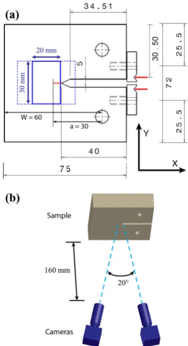
An experimental dataset was obtained using a fatigue pre-cracked Compact Tension (CT) specimen of an alu-minium (Al2024) alloy. The material was provided by Airbus Group as a 20 mm thickness plate in the T351 condition (i.e. solution heat treated and stress-relieved by stretching). The specimen dimensions, compliant with ASTM E399–09 [65], are specified on Fig. 2; the specimen thickness (B) is 20 mm and the orientation is LT. The Young’s modulus, E, of the tested material was measured to be 72.5 GPa ± 3 GPa using a resonance m e t h o d3 [6 6] w i t h a s a m p l e o f d i m e n s i o n s 71.7 × 20.0 × 3.67 mm; the value quoted in the litera-ture [67] for Al2024 is 73.1 GPa. The Vickers’hardness was determined at 146 ± 12 (standard deviation for 10 measurements); the literature value for the T351 heat treatment is 139 [67].

The specimen was fatigue pre-cracked at a frequency of 10 Hz at a load ratio (maximum/minimum load) of 0.1. Load shedding and optical observation on one surface

2_{ODIN–the MatLab code is available from the authors and can run with}

MatLab 2014a or higher.

maintained the maximum applied stress intensity factor below 15 MPa m0.5; this corresponds to 45% of the reported mode I plane strain fracture toughness,KIC, of 34 MPa m

0.5

for this alloy in the T351 heat treatment [67]. The pre-crack was prop-agated to an average depth of 4.95 mm from the notch tip (a range of ±0.25 mm was measured on either side of the sample after pre-cracking) to obtain a ratio a/W = 0.5 (i.e.

a/W= 0.499 ± 0.004 mm), whereais crack length andWis the specimen width (60 mm). The maximum load at the end of fatigue pre-cracking was 7.43 kN, which was applied over the final 1.5 mm of crack propagation. After pre-cracking, one surface of the sample was polished with grit-600 SiC paper and cleaned with ethanol. A non-reflective speckle pattern consisting of white and black spots was then applied using spray paint (Hammerite® smooth white & Rust-oleum® satin black) from a distance of ~1 m. A clip-gauge displacement transducer (Instron 2620–604 Extensometer, precision better than 0.1%) measured the crack mouth opening with load. The clip gauge was attached to knife-edges (thickness 7 mm) that

were mounted on the sample edge (Fig. 2(a)). The crack mouth opening displacement (CMOD) at the specimen sur-face was calculated from the clip gauge, using a correction coefficient obtained via a 3D linear elastic FE model of the test specimen for a crack depth a/W = 0.5. The simulated opening displacement at the location of the gauge for five different values of CMOD, with a least-squares linear fit (R2> 0.99), gave the clip gauge:CMOD ratio of 1:0.9752.

The stereo-DIC system comprised 2 CMOS Toshiba-Teli CSB4000CL-10A cameras, each capturing an image size of 2008 × 2047 pixels with a 10-bit depth. The cameras were positioned approximately 160 mm from the sample surface, on the same height with a 20° angle between cameras (Fig. 2(b)). With this set-up, the calibrat-ed pixel size was 15 μm on the re-projected images. Image acquisition was performed using an in-house LabVIEW code with 2 PCI-1428 acquisition cards, which allowed synchronized capture with timing accuracy better than 1 ms. Lighting was achieved using two 36-LED spotlights, with one placed above each camera. A 058–5 LaVision 3D calibration plate was placed on the surface of a test specimen that was positioned in the mechanical test frame (Instron 5982, with a 100 kN load cell). The DIC calibration, using the LaVision Davis 8.3.0 software, ap-plied the polynomial calibration algorithm and the obtain-ed re-projection error was less than 0.4 pixels for both cameras - the re-projection error is the mean difference between the positions of the calibration marks in the cal-ibration image and their known positions, after correction. The sample was loaded in a series of quasi-static cycles that progressively increased in magnitude up to 25 kN. A pre-load of 130 N was applied, and after each cycle the sample was unloaded to the same pre-load. Images were recorded at the maximum load and minimum load in each cycle. The DIC analysis of images was performed relative to both the pre-loaded reference state (‘extra-cycle’), and also to the min-imum loaded state at the end of the previous cycle (‘ intra-cycle’). In each case, the Step A analysis employed a square subset dimension of 32 pixels with an overlap be-tween subsets of 75%. A threshold correlation coefficient of 0.85 was used to censor the displacement vector re-sults; additionally, all vectors within 0.5 mm (equivalent to one subset size) of the crack path were censored. The step B analysis to detect the crack path used a square subset dimension of 9 pixels with 75% overlap. A straight crack was assumed and was fitted to the crack path, which was segmented from the step B strain data with a threshold that selected the top 1% of values of the max-imum normal strain histogram. The surface crack path and crack tip positions were subsequently verified by optical microscopy, and the crack front across the sample was examined by optical examination of the fracture surface after breaking open the sample at ambient temperature. Fig. 2 The experiment geometry: (a) CT specimen dimensions and

Results and Discussion

Synthetic Datasets

The relative error was evaluated between the J-integral obtained from the deformed images, and that calculated directly from the initial FE-model that had provided the input for the deformation of the images. As the position of the crack in the synthetic images is known precisely, the two-step DIC analysis was not required and it was sufficient to analyse the images with a single subset size to measure the displacement field. The effects on the J-integral of image noise and error in crack tip position were considered. In each case, the J-integral calculation was obtained for a set of different dimensions of the free region (P’Q’R’S′) in both horizontal and vertical direc-tions. A DIC analysis of the dataset was made using a subset of 64 × 64 pixels, with 75% overlap. As the crack tip position was known precisely, very good agreement was obtained between the J-integral that was calculated from the images and the original FE simulation; the rela-tive error varies from 0.06% to 0.3% when the SNR is infinite (i.e. no noise added). In the absence of added noise, varying the dimension of the free region in direc-tions both parallel and perpendicular to the crack has no significant effect on the J-integral error; in both cases free regions with dimensions of up to around 45 mm were examined. When the contours were taken within the free region, there was no measurable effect of applied image noise up to 15 dB, while the addition of extreme image noise (−5 dB) gave an uncertainty in the J-integral be-tween 0.8% and 2.7%. This analysis is for a crack loaded in pure mode I, and a greater sensitivity might be expect-ed with mixexpect-ed mode loading.

The J-integral analysis is therefore quite noise robust, so long as the contours remain within the free region where the fields are determined by the FE solution. The free region is mechanically connected to the surrounding full displacement field, so using contours that directly sample the DIC data, rather than those using displacements within the free region that is bounded by data, results in a loss of convergence if there is sufficient noise in the DIC data. This is illustrated in Fig.3, which considers the same free region size (P’Q’R’S′) and compares synthetic data with SNR of 96 dB and 45 dB. The distance of the outer contour from the crack tip is linearly proportional to the contour number, and the separation be-tween successive contours is 400μm; contours number 24 and above extend beyond the free region. The J-integral ob-tained for the contours beyond the free region for the 45 dB data does not converge, but for low levels of noise (i.e. SNR of 96 dB), the method performs well even for contours within the DIC data. A comparison with the JMAN method [41] that evaluates the J-integral directly from the DIC measurements

is also shown in Fig.3for a dataset with a SNR of 45 dB. The scatter is significantly reduced in the free region of the FE method, compared to the JMAN method.

The effect of uncertainty in the crack tip position is illus-trated using a DIC analysis with a subset of 64 × 64 pixels and an overlap of 75% for step A, with no noise added. Free regions with dimensions from around 20 to 45 mm were con-sidered, and the DIC results were injected into FE models in which the crack length was changed by up to ±50 pixels from its known position, equivalent to ±850μm or an error ina/W

of 1.4%. The obtained uncertainty is reported in Fig.4as the average error for the full range of free region sizes. There is no specific trend with the free region size, so the error bars are the standard deviation for all region sizes. The J-integral increases with the error in crack length, but remains low. In [34] the authors estimated a 7% average uncertainty in the determina-tion of the stress intensity factor by a field fitting method, for an uncertainty in crack tip position of 40 pixels. With the present method the error is of 3.8 ± 2.5% for a similar uncer-tainty in crack tip position.

Experimental Dataset

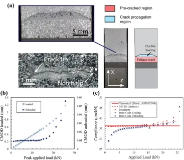
The surface trace of the crack and fracture surface are shown in Fig.5(a). The crack was straight and uniform within the ASTM E399–09 requirements [65]; the average crack surface length is 4.95 mm, measured on each side (±0.25 measure-ment precision) from the notch tip (a/W = 0.499), and the average crack length across the specimen was 5.19 mm (a/W= 0.503). The standard deviation of 5 evenly spaced measurements along the crack front was 0.12 mm, with a maximum length of 5.49 mm (a/W= 0.508). The crack mouth opening displacement (CMOD) is shown in Fig.5(b) for the loaded and unloaded condition as a function of the maximum applied load. The clip gauge was zeroed with the initially unloaded samples, before application of the 130 N pre-load. The loaded CMOD increases linearly with load until 20 kN load (i.e. applied K < 39 MPa.m1/2) and then rises more steep-ly. The unloaded CMOD, which is measured at 130 N, is approximately constant at 0.2 mm, but rises as the peak ap-plied load increases above approximately 15 kN (i.e. apap-plied K > 29 MPa.m1/2).

The specimen compliance data are shown in Fig.5(c) as a function of the maximum applied load. Several measures of compliance may be obtained from the data: the maximum complianceis calculated as the ratio of maximum CMOD to maximum applied load; theintra-cycle loading complianceis the ratio of the change in CMOD between the minimum and maximum load in each cycle to the applied load range; and the

standard [68] is 36.33μm/kN (±0.25). The uncertainty in the theoretical compliance is due mostly to uncertainty in the measured Young’s modulus; the measurement uncertainty in crack length make a negligible contribution. The maximum compliance is very close to the ASTM E399–09 theoretical compliance. Initially slightly lower (e.g. 1% difference at 2.5 kN), the maximum compliance increases gradually with in-creasing load up to about 15 kN, and then continues to rise at a rate that increases with increasing load. The intra-cycle load-ing and unloadload-ing compliances are almost identical and are initially lower than the maximum compliance. They approach the theoretical compliance as the maximum load increases, with the greatest changes occurring up to a maximum load of 7.5 kN and then above around 15 kN, where both increase significantly with applied load.

The DIC observations showed no measurable increase in crack length at the specimen surface, but ductile tearing and

blunting both occur sub-surface during the experiment, as indicated by the fracture surface (Fig.5(a)). An increasing in crack length by ductile tearing would increase both the intra-cycle unloading compliance and the maximum compliance, whereas crack blunting by plasticity would increase the load-ing compliance and the unloaded CMOD, with no significant effect on the intra-cycle unloading compliance. The reduced intra-cycle compliance below 7.5 kN may be attributed to plasticity-induced crack closure that was introduced by the fatigue pre-cracking. The effect of closure may also be appar-ent in the difference between the maximum compliance and the theoretical compliance at low loads. The increase in intra-cycle compliance above around 15 kN, accompanied by in-creased unloaded CMOD, can be attributed to crack tip plas-ticity. Above 24 kN, the difference between the unloading and loading intra-cycle compliance shows that plastic tearing to extend the average crack length has also occurred. Hence, the crack may be considered as fully open above approximately 7.5 kN, which was the maximum applied during fatigue-precracking. As the load increases above this, there is a pro-gressive increase in the crack tip plastic deformation, which becomes significant above 15 kN.

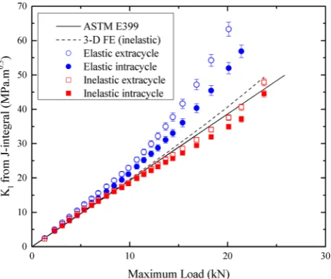
The ASTM E399 standard [65] was used to calculate the applied stress intensity factor, K, from the measured specimen dimensions, surface crack length and applied load. This is compared with a 3-D FE simulation for the same specimen dimensions, obtained using an inelastic Ramberg-Osgood model with the properties of Al2024-T351 (E= 73.1 GPa, ν= 0.33,σy= 325 MPa,n= 7.52,α= 1.31). The FE simula-tion assumed hard fricsimula-tionless contact between the loading pins and the sample, with displacement controlled boundary conditions at the loading pins to achieve the reaction forces Fig. 3 Illustration of the J-integral loss of contour independency that is caused by DIC noise when exiting the free region (around contour 25). The free region is included in the P’Q’R’S′box (a) Schematic representation of the contour numbers–contours 5, 20, and 30 are shown; contours 5 and 20 are included in the free region and contour 30 includes data out of the free region (b) Calculated J-integral value normalized by the theoretical value for different contours and different noise levels. Comparison is made with the JMAN method [41] for data with 45 dB SNR

equivalent to the applied load. The ASTM standard and FE simulation agree within 3% up to 15 kN applied load, above which the 3-D FE simulation increases non-linearly with in-creasing load due to plastic deformation. The FE simulation of the maximum CMOD agrees with the theoretical solution and also shows the effect of plasticity above 15 kN that is observed in the experimental data (Fig.5(c)). At higher loads, the mea-sured maximum compliance is greater than the inelastic FE simulation. This may be due to uncertainties in the FE model definition at large strains and also the development of tearing in the experimental data.

The DIC-measured surface displacement fields were used to calculate J-integral values (Fig.6(a)). A small subset anal-ysis (Fig.6(b)) was used to identify the crack position; the maximum normal strains values shown on the figure are un-filtered and their sole purpose is to determine the displacement discontinuity of the crack path by segmentation of the appar-ent strain field. The free region was fixed with dimensions of 6.4 × 3.1 mm. The J-integral calculation was performed with contours that were only within the free region. The experimen-tal noise from the image acquisition and 3D–DIC analysis prevented calculation of the J-integral for contours in the DIC data region, and the experimental data could not be analysed using the JMAN code [41] due to this noise.

For comparison with the ASTM standard calculation, the J-integral values were converted to stress intensity factors using

Equation 2, and are presented in Fig.7. Theextra-cycle anal-ysis used the displacement fields relative to the initial refer-ence 130 N preload, and the intra-cycle analysis used the relative displacement fields between the previous unload and the maximum load of each cycle. Each J-integral analysis was performed using linear elastic properties (plane stress, E = 73.1 GPa, ν = 0.3) and also the inelastic Ramberg-Osgood model for the Al2024-T351 alloy. The crack tip po-sition is known to within 15 pixels, and the maximum differ-ence between surface and average crack length was 240μm (i.e. 16 pixels), so the expected uncertainty in the evaluated J-integral for a correctly defined material law is approximately 1.5%. In the case of small scale yielding, where an elastic model is used instead of the correct inelastic model, an addi-tional bias of 5% is expected [62]. With the 4% uncertainty in Young’s modulus value, a propagation of error analysis gives an expected uncertainty in K of 2.2% when using the inelastic model and 3.2% when using an elastic model with the as-sumption of small scale yielding.

K¼

ffiffiffiffiffiffiffiffiffiffi

J*E0

p

Equation 2Mode I stress intensity factor calculation from J-integral result. E’= E for plane stress.

Fig. 5 (a) Optical microscopy of the surface crack and the fracture surface. The specimen surface in vicinity of the cracked region was cleaned with ethanol prior to taking the picture in order to remove the paint pattern applied for the DIC analysis. (b) The crack mouth opening

Figure7 shows that, with the assumption of small scale yielding (i.e. elastic behaviour), the extra-cycle DIC-based J-integral calculation obtains a higher stress intensity factor than the ASTM standard calculation. The standard analysis is rela-tive to a zero load rather than the 130 N preload, but the effect of this is vanishingly small, so the difference is largely due to the neglect of crack tip plasticity. Crack tip plasticity increases the displacements around the crack and so causes the strain energy close to the crack tip to be overestimated when the J-integral is calculated with the assumption of linear elasticity. This error increases at loads above 7.5 kN, since there is no significant development of crack tip plasticity below the fatigue pre-cracking maximum load. The intra-cycle elastic analysis shows a similar but smaller difference, as it is affected only by the plasticity that develops in individual cycles, rather than

the total plasticity. Crack closure, or the residual stress field associated with this, also has some effect, but it appears to quite complex; the difference between the extra-cycle and intra-cycle elastic J-integral analyses below 7.5 KN indicates that the dis-placement field around the crack is not simply linear elastic, despite the stability of the minimum CMOD that is observed in Fig.5(b). Incorporating the correct elastic-plastic material law into the J-integral analysis of the displacement field provides a better agreement between the applied and calculated stress in-tensity factor, particularly for the extra-cycle analysis that con-siders the total development of plasticity with increasing load. In this case, agreement to within 4.5% of the applied stress intensity factor is obtained, even when significant plasticity develops (i.e. above 15 kN load).

It is important to note that this J-integral analysis makes no use of the experimentally measured load, nor of the actual geometry of the test specimen. The analysis uses only the measured displacement field around the crack and an elastic or inelastic material law. The ASTM standard calculation re-quires knowledge of the specimen geometry, crack length and the applied load, and the assumption of small scale yielding. In the specimen geometry used here, the effects of crack tip plasticity on the ASTM standard calculation are not signifi-cant except at high loads, since the crack tip plastic zone is small compared to the specimen geometry and crack length. The image-based analyses show that the measured displace-ment field can be used to calculate the field applied to a crack, with good accuracy, without knowledge of the crack geometry and applied load. Significant errors arise only when crack tip plasticity is neglected.

The analysis uses the displacement field that is measured in the region surrounding the crack, but it is not immune to the effects of local effects close to the crack tip, such as the resid-ual stresses of crack closure that can influence the develop-ment of the displacedevelop-ment field. In principal, these local effects might be extracted by using displacements measured very Fig. 6 Example results of the

DIC analysis (at 15.5 kN); the origin of the x-y coordinates is at an arbitrary position; (a) y-displacement change measured for a large subset (64 × 64 pixels, overlap 75%) (b) maximum nor-mal strain obtained with snor-mall subsets (9 × 9 pixels, overlap 75%). The dashed boxes show the locations of the free region used in the J-integral analysis, and also the zoomed image of the crack. The position of the crack tip, ob-tained by segmentation of the strain data (small subset analysis) is also marked

local to the crack tip. However, convergence problems will occur due to noise in these data. Direct measurements of the crack tip field, such as via diffraction methods that record elastic strains, would be needed in this case. These can be analysed using a finite element-based methodology similar to that presented here, in order to characterise the local crack field that develops in response to an applied stress intensity factor (e.g. [69]).

Discussion

This paper has considered the means of obtaining the elastic strain energy release rate of a loaded crack either by direct calculation from the measured full-field displacements or indirect calculation from a FE-calculated field that is deter-mined by using the measured full-field displacements as a boundary condition. Both approaches calculate fields of strain and stress, which can then be analysed using the J-integral as presented herein or using field-fitting techniques.

The indirect-FE approach has the interest of being very robust to experimental noise, because the J-integral is calcu-lated over a region where the fields originate from the FE solution and are therefore essentially noise free. This is illus-trated in Fig.3(b), which shows no effect of image noise on the indirect-FE method for an applied noise of SNR 45 dB when the direct-FE approach (JMAN [41]) is seriously im-pacted by noise.

Direct field-fitting approaches, such as [32,34] have an insensitivity to noise as they calculate aBbest-fit^solution to the field, thus averaging the effects of noise over the dataset. In [34] it is demonstrated the dominant error in field-fitting comes from the unknown geometry of the crack (i.e. uncer-tainty in crack tip position), compared to displacement noise. This trend is demonstrated in Fig.4, where the J-integral error is constant for image noise lower than 15 dB SNR (very high noise level) but the crack tip position uncertainty induces more significant errors.

Direct-FE calculation of the J-integral, as exemplified by the JMAN approach or with the current method when the contours are taken out of theBfree^region, is per se theoret-ically insensitive to crack tip position as the integration con-tour does not need to contain the crack tip [40], but it is sen-sitive to experimental noise (Fig.3(b)), and so can only be successful with very good quality data. For instance, in Fig.3(b), the direct-FE evaluation is correct for an SNR of 96 dB but not feasible at 45 dB. A good image quality in an experiment would be expected to have SNR values between 40 dB and 60 dB.

It is possible to use smoothing of the data before field fitting in order to lower the field-fitting residuals [70], and a similar method could allow direct calculation of J-integral from smoothed experimental results, but this is less preferable

than using an indirect-FE calculation. This is because in the indirect approach, the smoothing of the effects of displace-ment noise is performed by the FE layer, so the calculation is informed by the material properties and continuum mechanics.

In the case of uncertainty or error in the material law, for instance when the measurements are made within the plastic zone, both direct and indirect techniques ex-perience issues. In the direct approach, measured strains are correct as they are derived from the displacement field but the calculated stresses would be erroneous. In the indirect-FE case, both strains and stresses in the FE regions are affected by the material law as they are determined from the displacement boundary conditions. However, they would be self-consistent with the im-posed material law and therefore would allow calcula-tion of a contour independent J-integral value. It is therefore important to correctly define the material law to obtain meaningful strain energy release rate values for indirect-FE calculation of the J-integral. Field fitting suffers the same problem, but with the additional draw-back that analytic solutions only exist for a limited number of material laws. The indirect-FE method dem-onstrated in this work can utilise any material law than can be described in the finite element simulation soft-ware Abaqus.

Conclusion

A method to determine the crack strain energy release rate from measured displacement fields has been presented, using digital image correlation (DIC) datasets. The method uses a Finite Element framework and is easy to imple-ment. The full-field DIC measurements are used to apply boundary conditions for finite element calculation of the J-integral. The method is insensitive to the specimen geom-etry, does not require prior knowledge of the loading and may be applied when DIC measurements in the vicinity of the crack are not trustworthy. The method has been benchmarked on synthetic datasets to assess the errors arising from uncertainty in crack tip position and image noise. Like any full field method, the choice of the mate-rial law must be considered carefully as it can be the major source of error. Application of the method to exper-imental data for an elastic-plastic material shows that the crack field (as a stress intensity factor) can be obtained with good accuracy, without knowledge of the specimen geometry and applied loads.

LaVision, Gmbh. SMB gratefully acknowledges the help and advice of Mr. Matthew S. L. Jordan, Mr. Matthew R. Molteno and Dr. L. Saucedo Mora. Data can be obtained from the corresponding author.

Compliance with Ethical Standards

Conflict of Interest Statement The authors certify that they have no affiliations with or involvement in any organization or entity with any financial interest, or non-financial interest in the subject matter or mate-rials discussed in this manuscript. They confirm that the paper consists of original, unpublished work, which is not under consideration for publi-cation elsewhere.

Open AccessThis article is distributed under the terms of the Creative C o m m o n s A t t r i b u t i o n 4 . 0 I n t e r n a t i o n a l L i c e n s e ( h t t p : / / creativecommons.org/licenses/by/4.0/), which permits unrestricted use, distribution, and reproduction in any medium, provided you give appro-priate credit to the original author(s) and the source, provide a link to the Creative Commons license, and indicate if changes were made.

References

1. Hutchinson JW (1968) Singular behaviour at the end of a tensile crack in a hardening material. J Mech Phys Solids 16:13–31 2. Rice JR (1972) Some remarks on elastic crack-tip stress fields. Int J

Solids Struct 8:751–758

3. Newman JC, Raju IS (1981) An empirical stress-intensity factor equation for the surface crack. Eng Fract Mech 15:185–192 4. Begley JA, Landes JD (1972) The J-integral as a fracture criterion.

Fract Toughness, ASTM STP 514:1–39

5. Wiederhorn SM, Boltz LH (1970) Stress corrosion and static fa-tigue of glass. J Am Ceram Soc 53:543–548

6. Brown BF, Beachem CD (1965) A study of the stress factor in corrosion cracking by use of the pre-cracked cantilever beam spec-imen. Corros Sci 5:745–748

7. Parkins RN (1980) Predictive approaches to stress corrosion crack-ing failure. Corros Sci 20:147–168

8. Newman JC, Wu XR, Swain MH et al (2000) Small-crack growth and fatigue life predictions for high-strength aluminium alloys. Part II : crack closure and fatigue analyses. Fatigue Fract Eng Mater Struct 23:59–72

9. Griffith AA (1921) The phenomena of rupture and flow in solids. Philos Trans R Soc London 221:163–198

10. Nishioka T, Atluri SN (1983) Analytical solution for embedded elliptical cracks, and finite element alternating method for elliptical surface cracks, subjected to arbitrary loadings. Eng Fract Mech 17: 247–268

11. Newman JC, Raju IS (1986) Stress-intensity factor equations for cracks in three-dimensional finite bodies subjected to tension and bending loads. In: Atluri SN (ed) Comput. Methods Mech. Fract. Elsevier Science Publisher, Amsterdam, pp 312–334

12. Irwin G (1962) Crack-extension force for a part-through crack in a plate. J Appl Mech 29:651–654

13. Luxmoore A, Light MF, Evans WT (1977) A comparison of energy release rates, the J-integral and crack tip displacements. Int J Fract 13:257–259

14. Zhu XK, Joyce JA (2012) Review of fracture toughness (G, K, J, CTOD, CTOA) testing and standardization. Eng Fract Mech 85:1– 46. doi:10.1016/j.engfracmech.2012.02.001

15. Suresh S, Zamiski GF, Ritchie RO (1981) Oxide-induced crack closure: an explanation for near-threshold corrosion fatigue crack growth behavior. Metall Trans A 12A:1435–1443

16. Elber W (1971) The significance of fatigue crack closure. Damage Toler Aircr Struct ASTM STP 486:230–242

17. Elber W (1970) Fatigue crack closure under cyclic tension. Eng Fract Mech 2:37–45

18. Liu S, Wheeler JM, Howie PR et al (2013) Measuring the fracture resistance of hard coatings. Appl Phys Lett 102:171907. doi:10.1063/1.4803928

19. Chiang FP, Asundi A (1981) A white light speckle method applied to the detemination of stress intensity factor and displacement field around a crack tip. Eng Fract Mech 15:115–121

20. Huntley JM, Field JE (1988) Measurement of crack tip displace-ment field using laser speckle photography. Eng Fract Mech 30: 779–790

21. Moutou Pitti R, Badulescu C, Grédiac M (2014) Characterization of a cracked specimen with full-field measurements: direct determina-tion of the crack tip and energy release rate calculadetermina-tion. Int J Fract 187:109–121. doi:10.1007/s10704-013-9921-5

22. Bruck HA, McNeill SR, Sutton MA, Peters WH (1989) Digital image correlation using Newton-Raphson method of partial differ-ential correction. Exp Mech 29:261–267

23. Chu TC, Ranson WF, Sutton MA, Peters WH (1985) Applications of digital image-correlation techniques to experimental mechanics. Exp Mech 25:232–244

24. Lu H, Cary PD (2000) Deformation measurements by digital image correlation: implementation of a second-order displacement gradi-ent. Exp Mech 40:393–400

25. Fazzalari NL, Forwood MR, Manthey BA et al (1998) Three-dimensional confocal images of microdamage in cancellous bone. Bone 23:373–378. doi:10.1016/S8756-3282(98)00111-2 26. Helm JD, McNeill SR, Sutton MA (1996) Improved

three-dimensional image correlation for surface displacement measure-ment. Opt Eng 35:1911–1920

27. Sutton MA, Reynolds AP, Yang B, Taylor R (2003) Mixed mode I/ II fracture of 2024-T3 friction stir welds. Eng Fract Mech 70:2215– 2234. doi:10.1016/s0013-7944(02)00236-9

28. Poncelet M, Barbier G, Raka B et al (2010) Biaxial high cycle fatigue of a type 304L stainless steel: cyclic strains and crack initi-ation detection by digital image correliniti-ation. Eur J Mech - A/Solids 29:810–825. doi:10.1016/j.euromechsol.2010.05.002

29. Rahimi S, Engelberg D, Duff JA, Marrow TJ (2009)In situ obser-vation of intergranular crack nucleation in a grain boundary con-trolled austenitic stainless steel. J Microsc 233:423–431

30. Kovac J, Alaux C, Marrow TJ et al (2010) Correlations of electro-chemical noise, acoustic emission and complementary monitoring techniques during intergranular stress-corrosion cracking of austen-itic stainless steel. Corros Sci 52:2015–2025. doi:10.1016/j. corsci.2010.02.035

31. Stratulat A, Duff JA, Marrow TJ (2014) Grain boundary structure and intergranular stress corrosion crack initiation in high tempera-ture water of a thermally sensitised austenitic stainless steel, ob-served in situ. Corros Sci 85:428–435. doi:10.1016/j. corsci.2014.04.050

32. McNeill SR, Peters WH, Sutton MA (1987) Estimation of stress intensity factor by digital image correlation. Eng Fract Mech 28: 101-112

33. Zhang R, He L (2012) Measurement of mixed-mode stress intensity factors using digital image correlation method. Opt Lasers Eng 50: 1001–1007. doi:10.1016/j.optlaseng.2012.01.009

35. Yoneyama S, Morimoto Y, Takashi M (2006) Automatic evaluation of mixed-mode stress intensity factors utilizing digital image correlation. Strain 42:21–29. doi:10.1111 /j.1475-1305.2006.00246.x

36. Bay BK, Smith TS, Fyhrie DP, Saad M (1999) Digital volume correlation: three-dimensional strain mapping using X-ray tomog-raphy. Exp Mech 39:217–226. doi:10.1007/BF02323555 37. Kirugulige MS, Tippur HV (2009) Measurement of fracture

param-eters for a mixed-mode crack driven by stress waves using image correlation technique and high-speed digital photography. Strain 45:108–122. doi:10.1111/j.1475-1305.2008.00449.x

38. Roux S, Réthoré J, Hild F (2009) Digital image correlation and fracture: an Advanced technique for estimating stress intensity fac-tors of 2D and 3D cracks. J Phys D Appl Phys 42:214004 39. Cherepanov GP (1967) The propagation of cracks in a continuous

medium. J Appl Math Mech 31:503–512

40. Rice JR (1968) A path independent integral and the approximate analysis of strain concentration by notches and cracks. J Appl Mech 35:379–386

41. Becker TH, Mostafavi M, Tait RB, Marrow TJ (2012) An approach to calculate the J-integral by digital image correlation displacement field measurement. Fatigue Fract Eng Mater Struct 35:971–984. doi:10.1111/j.1460-2695.2012.01685.x

42. Becker TH, Marrow TJ, Tait RB (2011) Damage, crack growth and fracture characteristics of nuclear grade graphite using the double torsion technique. J Nucl Mater 414:32–43. doi:10.1016/j. jnucmat.2011.04.058

43. Réthoré J, Gravouil A, Morestin F, Combescure A (2005) Estimation of mixed-mode stress intensity factors using digital im-age correlation and an interaction integral. Int J Fract 132:65–79. doi:10.1007/s10704-004-8141-4

44. Parks DM (1977) The virtual crack extension method for non linear material behavior. Comput Methods Appl Mech Eng 12:353–364 45. Shih CF, Moran B, Nakamura T (1986) Energy release rate along a

three-dimensional crack front in a thermally stressed body. Int J Fract 30:79–102

46. Pan B, Qian K, Xie H, Asundi A (2009) Two-dimensional digital image correlation for in-plane displacement and strain measure-ment: a review. Meas Sci Technol 20:62001. doi: 10.1088/0957-0233/20/6/062001

47. Duffy DE (1972) Moiré gauging of in-plane displacement using double aperture imaging. Appl Opt 11:1778–1781

48. Réthoré J, Hild F, Roux S (2008) Extended digital image correlation with crack shape optimization. Int J Numer Methods Eng 73:248– 272. doi:10.1002/nme.2070

49. Poissant J, Barthelat F (2009) A novel `subset splitting’procedure for digital image correlation on discontinuous displacement fields. Exp Mech 50:353–364. doi:10.1007/s11340-009-9220-2 50. Molteno MR, Becker TH (2015) Mode I-III decomposition of the

J-integral from DIC displacement data. Strain 51:492–503. doi:10.1111/str.12166

51. Yoneyama S (2011) Smoothing measured displacements and com-puting strains utilising finite element method. Strain 47:258–266. doi:10.1111/j.1475-1305.2010.00765.x

52. Kirugulige MS, Tippur HV, Denney TS (2007) Measurement of transient deformations using digital image correlation method and

high-speed photography: application to dynamic fracture. Appl Opt 46:5083–5096

53. Morton J, Post D, Han B, Tsai MY (1990) A localized hybrid method of stress analysis: a combination of moiré interferometry and FEM. Exp Mech 30:195–200. doi:10.1007/BF02410248 54. Tsai MY, Morton J (1991) New developments in the localized

hy-brid method of stress analysis. Exp Mech 31:298–305. doi:10.1007 /BF02325985

55. Caimmi F, Calabrò R, Briatico-Vangosa F et al (2015) J-integral from full field kinematic data for natural rubber compounds. Strain 51:343–356. doi:10.1111/str.12145

56. Pan B, Asundi A, Xie H, Gao J (2009) Digital image correlation using iterative least squares and pointwise least squares for dis-placement field and strain field measurements. Opt Lasers Eng 47:865–874. doi:10.1016/j.optlaseng.2008.10.014

57. Cinar AF, Tomlinson RA, Mostafavi M, et al (2015) Autonomous surface discontinuity detection method with digital image correla-tion. 10th Int. Conf. Adv. Exp. Mech.

58. Walters MC, Paulino GH, Dodds RH (2005) Interaction in-tegral procedures for 3-D curved cracks including surface tractions. Eng Fract Mech 72:1635–1663. doi:10.1016/j. engfracmech.2005.01.002

59. Williams ML (1952) Stress singularities resulting from various boundary conditions in angular corners of plates in extension. J Appl Mech 19:526–528

60. Williams ML (1957) On the stress distribution at the base of a stationary crack. ASME J Appl Mech 24:109–114

61. Rice JR, Rosengren GF (1968) Plane strain deformation near a crack tip in a power-law hardening material. J Mech Phys Solids 16:1–12

62. Barhli SM (2017) Advanced quantitative analysis of crack fields, observed by 2D and 3D image correlation, volume correlation and diffraction mapping. University of Oxford 63. Rooke DP, Cartwright DJ (1976) Compendium of stress intensity

factors. Procurement Executive, Ministry of Defence. H. M. S. O., London

64. Russ JC (2011) The image processing handbook, Sixth Edition doi:10.1201/b10720

65. American Society for Testing and Materials (1997) Standard test method for linear-elastic plane-strain fracture toughness of metallic materials. Annu B ASTM Stand 3(E):399–390. doi:10.1520/E0399-12E01.2

66. BSI (2007) Advanced technical ceramics—Mechanical properties of monolithic ceramics at room temperature

67. Bauccio M (1993) ASM metals reference book. ASM International 68. ASTM Standard E1820, ASTM (2013) Standard test method for measurement of fracture toughness. ASTM B Stand:1–54. doi:10.1520/E1820-13.Copyright

69. Barhli SM, Saucedo Mora L, Simpson C et al (2016) Obtaining the J-integral by diffraction-based crack-field strain mapping. Procedia Struct Integr 2:2519–2526