Identification of geometrical models of interface evolution for dendritic crystal growth

This is a repository copy of Identification of geometrical models of interface evolution for dendritic crystal growth.

White Rose Research Online URL for this paper: http://eprints.whiterose.ac.uk/74662/

Monograph:

Zhao, Y., Coca, D., Billings, S.A. et al. (2 more authors) (2010) Identification of geometrical models of interface evolution for dendritic crystal growth. Research Report. ACSE

Research Report no. 1011 . Automatic Control and Systems Engineering, University of Sheffield

[email protected] https://eprints.whiterose.ac.uk/ Reuse

Unless indicated otherwise, fulltext items are protected by copyright with all rights reserved. The copyright exception in section 29 of the Copyright, Designs and Patents Act 1988 allows the making of a single copy solely for the purpose of non-commercial research or private study within the limits of fair dealing. The publisher or other rights-holder may allow further reproduction and re-use of this version - refer to the White Rose Research Online record for this item. Where records identify the publisher as the copyright holder, users can verify any specific terms of use on the publisher’s website.

Takedown

If you consider content in White Rose Research Online to be in breach of UK law, please notify us by

Identification of Geometrical Models of Interface Evolution for

Dendritic Crystal Growth

Y. Zhao, D.Coca, S.A. Billings, R.I.Ristic, L.L.De Matos

Research Report No. 1011

Department of Automatic Control and Systems Engineering The University of Sheffield

Mappin Street, Sheffield, S1 3JD, UK

Identification of Geometrical Models of Interface Evolution for Dendritic

Crystal Growth

Y.Zhaoa, D.Cocaa, S.A.Billingsa, R.I.Risticb, L.L.De Matosb

a

Department of Automatic Control and System Engineering, University of Sheffield, UK, S1 3JD

b

Department of Chemical and Process Engineering, University of She eld, UK, S1 3JD.

Abstract

This paper introduces a method for identifying geometrical models of interface evolution, directly from experimental imaging data. These local growth models relate normal growth velocity to curvature and its derivatives estimated along the growing interface. Such models can reproduce many qualitative features of dendritic crystal growth as well as predict quantitatively its early stages of evolution. Numerical simulations and experimental crystal growth data are used to demonstrate the applicability of this approach.

Key words: dendritic crystal growth, geometrical models interface evolution, curvature-driven growth

1. INTRODUCTION

There is considerable technological and scientific interest to understand and manipulate pattern formation in

systems that evolve far-from-equilibrium. Complex patterns formed under far-from-equilibrium conditions are

encountered in a wide range of systems including hydrodynamical, chemical and biological systems. A large

number of such patterns are the result of the growth of an interface between two domains driven by two or

more competing fields.

An important example of such interfacial pattern formation, arising from the interplay between kinetic growth

and surface tension, is that of dendritic crystal growth. Over the past decades, a lot of effort has been directed

towards the development of mathematical models of interfacial crystal growth. Depending on whether the

interfacial motion is solely the result of local processes or involve long range diffusional processes, crystal

growth models can be divided into local models and more sophisticated non-local evolution models, which take

into account temperature and/or concentration fields.

Local models of dendritic crystal growth include cellular automata-type models1-4, diffusion-limited

aggregation (DLA) models5 and geometric models6-10, which describe interfacial growth velocity in terms of

the geometric properties of the phase boundary, typically curvature. Of the models that take into account

long-range diffusional effects, phase field models11,12 are perhaps the most popular and widely used.

Whilst numerical computations of dendritic growth can provide extremely realistic simulations of this complex

phenomenon, which can reproduce qualitatitively the observed behaviour, a major challenge is fine tuning the

model equations in order to achieve quantitative agreement between the computed solution and experimental

data.

This paper introduces an approach for inferring the structure and parameters of geometric models of dendritic

crystal growth directly from experimental imaging data. Although geometrically motivated models for

interfacial growth cannot replace detailed evolution models that can predict the long-term dynamics of the

system, it has been shown7-9 that local geometric models can capture the most interesting features of the pattern

formation and thus can provide valuable information of the underlying mechanisms of crystal growth.

The reminder of the paper is organized as following. Section 2 introduces the geometrical model of interface

evolution. Section 3 presents the image processing techniques used to extract basic quantities required for

model development, the methodology for estimating the model based on the resulting data set and the

application of the proposed modelling approach to synthetic data as well as experimental imaging data of

NH4Br growth. Finally, Section 4 summarizes the results.

2. GEOMETRIC GROWTH MODEL

Geometrical models of interface evolution are a class of local models that have been introduced, in a series of

papers6-9, as an alternative to global models of two-phase systems.

Essentially, geometrical models reduce the dynamics of a two-phase system evolving in a d-dimensional space

to an evolution equation for the interface which relates the normal component of interface velocity to local

geometric properties of the interface, namely curvature and its derivatives.

In two dimensions, at a time t, the crystal is assumed to occupy an open subset Ωt∈IR2 with boundary

represented by an evolving closed curve (t) separating its interior and exterior.

A planar closed curve is a map :[0,S) × (0, T) IR2 such that (s,t)=(x(s,t),y(s,t)) is a point on the curve (t)

and (0,t)= (S,t). The curve is parameterised so that the interior is on the left in the direction of increasing s

(counter clockwise parameterisation). The unit tangent to the curve is and the unit normal, pointing

inside the curve, is , where denotes the norm of denotes the inner

product of and , and .

Curvature can be defined as the amount of the degree of bending of a mathematical curve, or the tendency at

For a plane curve the signed curvature is given by

where denotes the determinant of the 2×2 matrix with column vectors and . According to Frenet’s

formulae, and .

The sign of the curvature k(s) indicates the direction in which the unit tangent vector rotates as s increases

along the curve. If the unit tangent rotates counter clockwise, then k > 0; otherwise k < 0 i.e. the curvature of a

circle is positive.

As the crystal grows, its boundary generates a family of curves { (t), t∈ [0, T)}. The velocity of the interface

(t) is given by

where V is the normal velocity and V is the tangential velocity. Here it is assumed that the growth interface

propagates with curvature dependent speed. Specifically the normal velocity is assumed to be a function of

curvature k and orientation angle θ

where θ is defined by cos . The tangential velocity has no effect on the shape of evolving curve so

usually V=0. The dependence of normal velocity on the curvature is related to interfacial free energy and

surface tension effects on the interface whereas the dependence on the orientation of the interface captures

anisotropic effects.

The case when V is linear corresponds to the classical mean curvature flow. This simpler model is suitable for

describing very slow growth. In general however, the dependence of V on the curvature is highly nonlinear.

In the case of dendritic crystal growth, Brower et al.7 (1984) proposed the following geometric model

cos (1)

where α represents the degree of undercooling, β is related to the minimum bubble size for nucleation and

is a ‘surface tension’ term. The term proportional with reflects crystalline anisotropy.

Numerical studies8 have demonstrated that such relatively simple model can reproduce many important

macroscopic features of dendritic growth when the long range effects (diffusion, heat flow etc) are not

significant, such as in the early stages of pattern formation,.

The model can be extended to incorporate global effects by coupling (1) with an evolution equation for the

3. Estimation of Geometrical Evolution Laws from Data

The problem addressed here is that of inferring the geometric model of crystal growth (1) directly from real

time observations. Besides the pure theoretical interest in interfacial pattern formation, there is a lot of interest

in controlling the size and the shape of a crystalline product by manipulating the temperature, concentration or

by the introduction of specific additives. In this context, the systematic design and implementation of an

automatic control system for regulating crystal morphology would require a mathematical model of the process

which captures not only the qualitative aspects of the dynamics but also the relevant physical parameters of the

process, which may be time-varying. For a particular application, the development of such a model based solely

on first principles calculation is very challenging if not impossible. Deriving accurate parameter information

requires experimental data and parameter estimation techniques.

While a detailed global model would provide a more accurate representation of the process this is achieved at

the expense of a significant computational burden which is not necessarily justified in a specific theoretical

study or practical application. As demonstrated in Kessler et al9 (1985) local geometrical models provide a

very useful tool for theoretical analysis and characterization of dendritic growth. On the other hand, in a

practical model-based control application involving real-time monitoring of growth patterns, by updating the

local model parameters in real-time, it should be possible to mitigate for the shortcomings of the model, such as

the absence of long range diffusional effects.

3.1 Experimental Data Acquisition and Pre-processing for Geometric Feature Extraction

In this study, 2D dendrite growth patterns of NH4Br crystals were recorded over time using a CCD camera

connected to a standard PC. The camera was mounted onto a stereographic microscope focused on the NH4Br

sample that was placed on a temperature-controlled stage. Back lighting was introduced underneath the glass

stage in order to illuminate and enhance the contrast of the solidifying structure against the surrounding liquid

media. High quality snapshots were recorded using the CCD camera which, when operating at full speed, could

record 25 fps (frames per second) with 800 × 600 resolution. The actual sampling rate was set so that the tip

speed of the fastest growing part of the crystal was roughly one or two pixels per time step. Typically, the

sampling rate was one frame or half a frame per second. A detailed description of the experimental setup can be

found in Zhao et al4 (2004).

The recorded 2D images of dendritic crystal growth were subsequently processed to extract curvature and

velocity measurements along the solid-liquid interface. The initial processing step involves filtering the images

to reduce measurement noise. In the next stage, image segmentation was performed on every image to separate

the crystal from the background. This resulted in a binary image in which the pixels corresponding to the object

and background are encoded as ‘1’s and ‘0’s respectively. To the resulting binary image was subsequently

solid-liquid interface.

Traditionally, curvature of a point on a discrete curve can be obtained by finding a circle that ”fits” the curve at

that point. Given any curve and a point P on it where the curvature is non-zero, there is a unique circle which

most closely approximates the curve near P, the so called osculating circle at P. The reciprocal of the radius

osculating circle is defined as the curvature of the considered point. If the centre of the fitted circle is inside the

curve, the curvature is positive, otherwise is negative.

Let P(i,t) be a point that corresponds to the i-th point in the coordinate list of the crystal interface extracted

from an image at time t. The curvature at this point was calculated by fitting a circle to three points P(i-h,t) ,

P(i,t), P(i+h,t). The curvature k(i,t) is approximated by the reciprocal radius of the fitted circle

In practice the accuracy of the resulting curvature is dependent on the chosen value for h.

Theoretically, the smaller h is, the more accurate the calculated curvature is. However, for smaller values of h,

the effect of measurement/quantisation noise can distort the results considerably. In practice, it is very

important to find an appropriate value for h which results in relatively accurate estimation of the curvature in

the presence of noise. Moreover, the optimal value for h is not constant along the boundary. For large

curvatures the value of h should be smaller than the value used for large curvatures. As the curvature is not

known a priori, a two-step method for curvature calculation was developed and used in this study. The method

was first tested using synthetic data generated for the following curve

Essentially the curvature for every boundary point was calculated twice. In the first instance a fixed value for h

was used to compute an initial rough estimate of curvature . In the second stage, the curvature was

re-calculated using a curvature-dependent h. The mapping h( ) used in this stage is illustrated in Figure 1b, with

the initial and re-assigned curvature (for the curve in Figure 1a) shown in Figure 1c.

[Insert Figures 1 about here]

The advantage of this approach is illustrated in Figures 1d which show the theoretical and computed curvatures,

using fixed and curvature-dependent h, for a known closed curve.

The arc-length (natural) parametrization of the curve is obtained by substituting the index i of every point P(i,t)

and k(i,t) in the coordinate list for s, the approximate arc length of the curve starting in P(1,t) and ending in

P(i,t), which is obtained using a pixel-based estimation approach for a pixel size of 2.13µm, calculated based

on the real size of the image.

derivatives , . In this work, higher order derivatives of k(s,t) were calculated by first fitting the

estimated curvature using a quintic smoothing spline.

The centre of the osculating circle fitted at point , denoted here by

, lies on the normal line at the point . The angle corresponding to the normal vector

to the curve in is therefore given by

arctan

Let ∆ ∆ ∆ be the intersection of the normal line evaluated at on

the curve γ(t) with the curve γ(t+∆ ). The normal velocity at is then approximated as

∆

3.2 Model Estimation

Two cases are considered here. In the first case the structure of the model is know and only the model

parameters need to be estimated. The second case, investigates the estimation of both model structure and

parameters.

Consider again the two-dimensional local interface model7,8

cos (2)

where α=1, β=-0.25, δ=1 and ε=0 (no anisotropy).

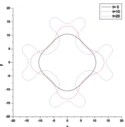
The model was simulated numerically using as initial conditions, a perturbed circle

sin

where is the arclength of a circle of radius . The resulting evolving spatial pattern, which is

displayed in Figure 2, resemble the early growth stages of cyclohexanol crystals shown in Ovisienko et al.13.

To evaluate the algorithms for computing curvature and normal growth velocity from data, tip speed and

corresponding curvature samples were generated with sampling time ∆t=0.0022.

[Insert Figure 2 about here]

Assuming that the model structure was known, the coefficients were estimated by ordinary least squares. The

which demonstrates the applicability of the image segmentation and geometric feature extraction algorithms.

In practice however, it is not always possible to postulate precisely the local equations of motion for a

particular crystal growth experiment.

Assuming that the normal growth velocity is a polynomial function of curvature and its derivatives,

where, for a given polynomial order n, not all polynomial terms are present, the problem is to select the relevant

polynomial model terms that describe the underlying growth dynamics.

This model structure selection task was performed using an Orthogonal Forward Regression algorithm14.

Essentially, the candidate model terms are ranked based on their contribution, known as the Error Reduction

Ratio (ERR), to reducing the variance of the dependent variable. The terms are selected iteratively in a

forward manner so that the best model term (largest ERR contribution) of all candidate model terms

(monomials of degree up to n in k and higher order derivatives). The remaining candidate terms in the model

set are orthogonalized with respect to the currently selected model subset, after every iteration step.

This approach was employed to estimate a geometric evolution model based on 2D dendrite growth patterns of

NH4Br crystals obtained experimentally, as detailed in section 3.1.

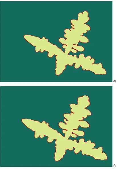
Figures 3a-c show three raw images of the crystal recorded at different time points (∆t, 20∆t, 40∆t where

∆t=3seconds) whilst the corresponding segmented images and identified boundaries are shown in Figures 3d-f.

Strictly speaking the crystal has a 3D structure but in this case it is believed that a 2D model provides a good

approximation of the growth dynamics as the NH4Br solution in this experiment is sandwiched between a

circular microscope slide and the optical window of the glass stage, using a thin strip of mylar as a separator4.

[Insert Figures 3 about here]

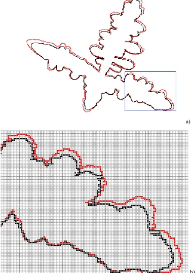
In order to minimise the effects of crystalline anisotropy, only the bottom-right branch of the crystal, as shown

in Figures 4a,b was analysed. The approach however could be extended to address anisotropy, in which case

velocity-curvature data for the entire boundary could be used to derive the model.

[Insert Figures 4 about here]

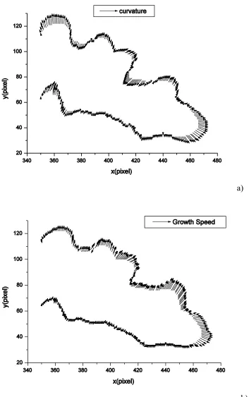
The curvature and normal velocity along the boundary were computed using the algorithms described earlier.

Figures 5a,b illustrate the curvature and normal velocity estimated along the branch of interest at frame 22.

[Insert Figures 5 about here]

The second order derivative of the curvature with respect to arclength s, starting from the top left corner of

Figure 4bisillustrated in Figure 6.

[Insert Figure 6 about here]

Model Term ERR 1 0.83685 0.08555 0.00558 0.00303 0.00071 0.00033

Only the first four terms, with a total ERR of 0.93, were considered significant and selected in the final model.

The resulting estimated model is given by

The presence of a constant term in the model indicates that, in this crystal growth experiment, the zero

curvature (planar) interfaces are not static.

The estimated model was used to generate predictions over entire crystal boundary, using the crystal boundary

in frame 1 as initial condition. Figure 7, which shows the initial crystal boundary in frame 1 and the predicted

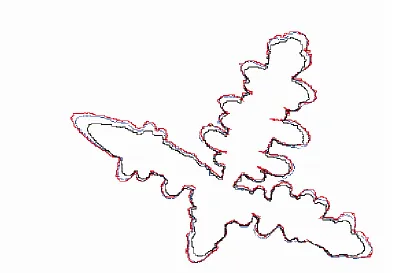
and the observed boundary in frame 42, demonstrates that the simple geometric model inferred from

experimental imaging data was able to capture the underlying growth characteristics of the crystal.

[Insert Figure 7 about here]

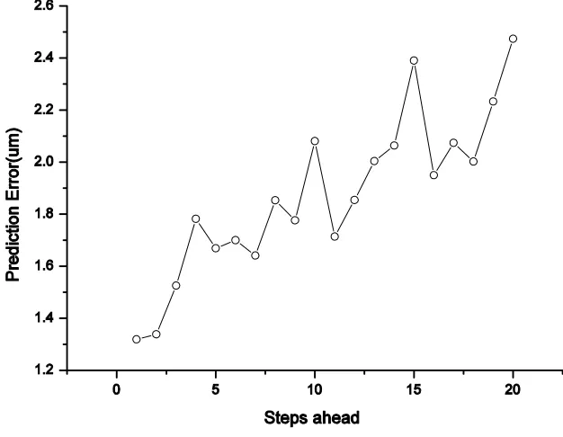
The prediction errors at time t were calculated using the formula

where S is the number of prediction points on the boundary. The prediction errors for different prediction

horizons are illustrated in Figure 8. As expected, the prediction error increases with prediction horizon, mainly

driven by the crystal anisotropy which was not taken into account by the current model but also due to the

inherent limitation of geometric models which do not account for long range interactions which become

significant on longer time scales. Although not perfect, the model could provide a good basis for the

implementation of model based control strategies, particularly in cases when theoretical models are difficult to

derive or their complexity makes them unsuitable for real-time control implementation.

To mitigate for the inherent limitation of geometric models, the model parameters could be updated on-line

using recursive estimation techniques.

4. Conclusions

This paper introduced for the first time a technique for the identification of geometric models for interfacial

growth of dendritic crystals directly from time lapse imaging data. Geometric models reduce the dynamics of a

two-phase system to a local geometric evolution equation in which the normal interface velocity is determined

by curvature and its derivatives.

Although such models cannot capture long-range diffusive processes which, for example, account for the

growth competition between dendritic fingers, local geometric models can reproduce8,9 the Mullins-Sekerka

instability15, the classical Ivantsov solution16 and many other qualitative features of dendritic growth.

The models can be used to make quantitative predictions, particularly during early stages of crystal growth or

over shorter time scales when nonlocal effects can be ignored. Due to their simplicity, these models could be

particularly useful for implementing advanced real-time model-based control strategies for crystal growth

processes. The use of phase-field models in this context is limited by the significant computational effort

required, particularly when investigating dendritic growth, and by the large number of parameters involved in

the solution of the evolution equations, which are difficult to determine to obtain sufficiently accurate model

predictions.

References

[1] Eden, M. A two-dimensional growth process. 4th. Berkeley symposium on mathematics statistics and

probability, 4:223–239, 1956.

[2] Packard, N. H. Lattice models for solidification and aggregation. In: Wolfram S, editor. Theory and applications of cellular automata. World Scientific Publishing, Singapore: 305-310, 1986.

[3] Zhao,Y., Billings, S.A. and Coca, D. Cellular automata modelling of dendritic crystal growth based on Moore and Von Neumann neighbhourhoods. International Journal of Modelling, IdentiÞcation and Control, 6(2):119-125, 2009.

[4] Zhao,Y., Billings, S.A., Coca, D., Ristic, R.I. and De Matos, L. Identification of the transition rule in a modified cellular automata model: the case of dendritic NH4Br crystal growth. International Journal of

Bifurcation and Chaos, 19(7):2205-2305, 2009.

[5] Witten, T.A. and Sander, L.M. Diffusion limited aggregation. Physical Review B, 27(9):5686-5697,1983.

[6] Ben-Jacob, E, Goldenfeld, N, Langer, J.S., and Schon, G. Boundary-layer model of pattern formation in solidification. Physical Review A, 29:330-340, 1984.

[7] Brower, R. C., Kessler, A. D., Koplik J.and Levine, H. Geometrical models of interface evolution,

Physical Review A, 29:1335-1342, 1984.

Simulation, Physical Review A, 30:3161-3174, 1984.

[9] Kessler, A. D., Koplik J.and Levine, H. Geometrical models of interface evolution. III. Theory of dendritic growth, Physical Review A, 31:1712-1717, 1985.

[10] Wettlaufer, J.S., Jackson, M and Elbaum, M. A geometric model for anisotropic crystal growth.

J. Phys. A: Math. Gen. 27:5957-5967, 1994.

[11] Kobayashi, K. Modeling and numerical simulations of dendritic crystal growth. Physica D,

63:410-423, 1993.

[12] Chen, L-Q. Phase-field models for microstructure evolution. Annu. Rev. Mater. Res. 32:113-140, 2002.

[13] Ovsienko, D.E, Alfintsev, G.A and Maslov, V.V. Kinetics L/kT values. Journal of Crystal Growth, 26(2):233–238, 1974.

[14] Billings, S.A., Chen, S. and Kronenberg, M.J. Identification of MIMO nonlinear systems using a forward-regression orthogonal estimator, Int. J. Contr., 49:2157–2189, 1989.

[15] Mullins, W.W. and Sekerka R. W. Morphological Stability of a Particle Growing by Diffusion or Heat Flow, Journal of Applied Physics 34:323-329, 1963.

[16] Ivantsov, G.P. Temperature field around spheroidal, cylindrical and acicular crystal growing in a supercooled melt. Dokl. Akad. Nauk SSSR 58:567-569, 1947

List of Figures

b)

d)

Figure 1. a) Simulated curve evolution. b) Mapping used to re-assign h according to estimated curvature; c) Initial h (dashed) and re-assigned h (solid) ; d) Comparison of curvatures computed using fixed and variable h

for given curve.

a)

c)

e)

f)

a)

b)

a)

b)

Figure 6. Derivative of curvature with respect to arclength.

Figure 7. Original boundary in frame 42 (blue) and model predicted boundary (red) given, as initial conditions,