Time-varying Models for Macroeconomic Forecasts

(1)

Time-varying Models for

Macroeconomic Forecasts

Bo Zhang

A thesis submitted for the degree of

Doctor of Philosophy at

The Australian National University

(2)

(3)

Except where otherwise indicated, this thesis is my own original work.

Bo Zhang

(4)

(5)

(6)

(7)

Acknowledgments

First, I would like to express my deep appreciation to my supervisors, Dr. Joshua

Chan, Dr. Timothy Kam, Dr. Shaun Vahey, and Dr. Rodney Strachan for their inspiring discussion during my study at the Australian National University (ANU), and

their invaluable academic advice on my thesis. I want to thank Prof. Joshua Chan for

spending so much time on my research discussion. He provided valuable advice on the topic selection, academic writing, and economic understanding of my thesis. Without

his supervision, I would not have mastered the necessary research tools or developed

a good understanding of the economy, and my thesis would not have reached a high standard. I would like to thank Dr. Timothy Kam for his dedication to my thesis

over the past year. Without his support, I would not have been able to continue the

second half of my PhD study so smoothly. I also want to thank Dr. Shaun Vahey for his academic inspiration on my thesis topic. His warm encouragement of my research

proposal also provided me with the invaluable opportunity to study at ANU. I would

like to thank Dr. Rodney Strachan for kindly joining the panel as one of my co-supervisors. His wide-ranging academic discussions broadened my economic research

horizons and showed me how to do my research well.

I want to thank Dr. Renee Fry-Mckibbin, Dr. Tue Gorgens, Dr. Bob Gregory, Dr. Kieron Meagher, Dr. Dennis Richard, and Dr. Ronold Stauber for helping me lay a

solid academic foundation. I would also like to express my thanks to other academic and administration staﬀ for their kind support during my research life at ANU.

Financial support provided by an ANU Australian Postgraduate Award is gratefully

acknowledged.

I want to thank my friends Jim Hancock, Dr. Zhongying Sun, Xin Zhang, and

Jamie Cross for polishing the English of my papers. I also wish to thank Xu Yang,

Chenghan Hou, Wenjie Wei, and Yaqing Zhang for their challenges and for sharing knowledge. Editing services were provided by professional editors from Elite Editing.

Finally, I would like to express my sincere appreciation to all my family members

for their patience, understanding, and both spiritual and material support while I undertook my PhD study.

(8)

(9)

Abstract

This thesis consists of three studies focusing on ways to detect and model time

variation among macroeconomic variables. In these three studies, errors with

autore-gressive moving averages (ARMA), model averaging, and stochastic volatility (SV) are used to investigate the uncertainty and the instability of macroeconomic dynamics.

In particular, I expand upon both univariate (autoregressive; AR) and multivariate

(vector autoregressive; VAR) time series models.

Chapter 1 provides a general introduction to the research interest of this thesis.

Next, Chapter 2 introduces an ARMA component with SV into the unobserved

com-ponent model. A transformation to a stacked matrix form of the model is conducted for posterior fast simulation. The proposed model is then used to study

macroeco-nomic time series in the United States (US). The proposed new model provides good

full-sample simulation for the majority of the macroeconomic variables, and can im-prove both the point and the interval forecasting performance of these variables across

diﬀerent horizons.

In Chapter 3, I use real-time macroeconomic variables and both time-varying and equal weights with time-varying parameter models to forecast inflation in the US. Three

time-varying coeﬃcient models with three specifications of their error terms are

stud-ied. The alternative error-term assumptions are errors with a Gaussian distribution, errors with SV, and errors with moving average SV. Both point forecasts and density

forecasts suggest that adding variables and allowing time-varying lag length choice

can significantly improve forecasting performance. The forecasting performance of the time-varying and equal weights model combination methods show that adding SV can

improve density forecasts but not point forecasts.

Finally, in Chapter 4, I employ a time-varying parameter VAR with SV (TVP-VAR-SV) to analyze the dynamics of renewable electricity generation (REG), gross

domestic product (GDP) growth, and CO2 emissions. TVP-VAR-SV and other re-stricted variants are employed for forecasting REG with data from the US. The

em-pirical results suggest that TVP-VAR-SV is suitable for studying the relationship

between REG, GDP, and CO2. The forecasting results suggest that VARs with a time-varying volatility specification can perform much better than those without SV, while

allowing for time-varying coeﬃcients does not improve forecasting performance.

(10)

(11)

List of Figures

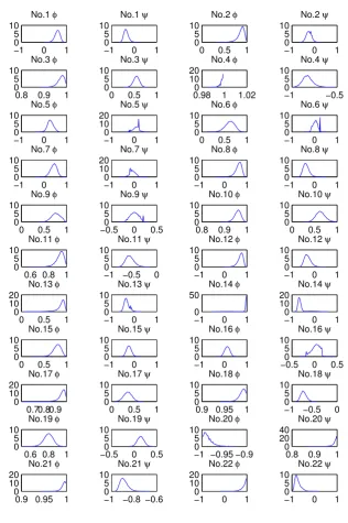
2.1 Marginal probability estimates for ϕand ψunder UC-ARMAmodels. 26

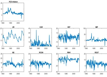
3.1 PCE inflation and inflation predictors. . . 49

3.2 Posterior estimates of TVC-SVMA where the predictor is the UR. . . 50

3.3 Posterior estimates of TVC-SVMA where the predictor is CUR. . . . 52

3.4 Posterior estimates of TVC-SVMA where the predictor is HSTS. . . . 52

3.5 Posterior estimates of TVC-SVMA where the predictor is IMP. . . 53

3.6 Posterior estimates of TVC-SVMA where the predictor is M2. . . 53

3.7 Posterior estimates of TVC-SVMA where the predictor is RCON. . . 54

3.8 Posterior estimates of TVC-SVMA where the predictor is RINV. . . . 54

3.9 Posterior estimates of TVC-SVMA where the predictor is ROUT. . . 55

3.10 Weights of component models forTVC, forecasting horizon one. . . . . 62

3.11 Weights of component models forTVC, forecasting horizon four. . . . . 69

3.12 Weights of component models forTVC, forecasting horizon eight. . . . 69

3.13 Weights of component models forTVC, forecasting horizon sixteen. . . 70

4.1 Plot of REG growth rate. . . 76

4.2 Plot of annualized real GDP growth rate. . . 77

4.3 Plot of CO2 emission growth rate. . . 77

4.4 SD of posterior medians for C-VAR-SVand TVP-VAR-SV. . . . 81

4.5 One-quarter-ahead cumulative sum of LPL for VAR models relative to AR(1) with one lag (left panel) and two lags (right panel). . . 85

4.6 One-quarter-ahead cumulative sum of CRPS for VAR models relative to AR(1) with one lag (left panel) and two lags (right panel). . . 86

(16)

(17)

List of Tables

2.1 Variables used in model comparison. . . 16

2.2 The number and percentage of the best models with diﬀerent error spec-ifications based on MSFE for 22 macroeconomic variable forecasting. . . 19

2.3 The number and percentage of the best models with diﬀerent model group specifications based on MSFE for 22 macroeconomic variable fore-casting. . . 20

2.4 The number of the best models based on MSFE for 22 macroeconomic variable forecasting. . . 20

2.5 The number and percentage of the best models with diﬀerent error spec-ifications based on RelLPL for 22 macroeconomic variable forecasting. . 21

2.6 The number and percentage of the best models with diﬀerent model group specifications based on RelLPL for 22 macroeconomic variable forecasting. . . 22

2.7 The number of the best model for each specification based on LPL for 22 macroeconomic variable forecasting. . . 22

2.8 The modes ofϕand ψin models withARMA-SVerrors and the mode of ψ in theUC-MA model. . . 24

3.1 Real-time forecasts for PCE inflation. . . 60

3.2 Correlation coeﬃcients between inflation predictors. . . 62

4.1 Sum of MLL and CRPS for the fitness of VARs. . . 80

4.2 SD with 16th and 84th quantiles for TVP-VAR-Cand C-VAR-C. . . 83

4.3 Relative average LPL and CRPS for REG forecasts from 1995. . . 84

(18)

(19)

Chapter 1

Introduction

In macroeconomic empirical research, the movement of economic variables attracts

strong interest from researchers. To reveal the evolution of these macrovariable time series, both univariate and multivariate frameworks with many time-varying

specifica-tions have been considered in studies. The present thesis contributes to the literature

by modeling these time series with time-varying features. Specifically, the correlation of error terms, model averaging, time-varying parameters, and stochastic volatility

(SV) are highlighted in the three main chapters. After evaluating the in-sample

fit-ness of the proposed models, the results of out-of-sample forecasts are reported in the “Application” section. The empirical parameter simulation and modeling evaluation

in this thesis are conducted by Bayesian econometrics. Both a block-banded sparse matrix and a precision-based algorithm are used for the rapid and eﬃcient simulation

of parameters.

Chapter 2 introduces SV with autoregressive moving average (ARMA; SV-ARMA) errors in the univariate unobserved components (UC) model. Another contribution of

this thesis is that it is the first study to run forecasts on United States (US) macrovari-ables with SV-ARMA error terms. Other competing models include UC models with or

without error correlation and SV assumptions; moreover, some simple but hard to beat

univariate models, such as random walk (RW) and AR models, are also considered. In this chapter, both point and interval forecasting results are presented, and the analysis

of forecasting performance is based on 22 quarterly macroeconomic time series with 13

modeling specifications allocated in four groups.

Chapter 3 focuses on inflation forecasts. Inflation is a core macroeconomic indicator

and has received considerable attention from both central bankers and macroeconomic researchers. In this chapter, model averaging time-varying weight and equal weight

strategies are considered for either point forecasts or density forecasts with eight

infla-tion predictors. The modeling competiinfla-tion is conducted using UC models with SV and SVMA errors, with dynamic model averaging and selection for these highly competitive

models.

(20)

Chapter 4 employs a time-varying parameter vector autoregressive (TVP-VAR)

model with SV to investigate the relationship between the renewables, output, and CO2 emissions. In fact, TVP-VARs are already widely accepted and applied to

macroeco-nomic studies to investigate the dynamic interactions between variables. The empirical

results indicate that the SV specification shows a better fitness to the data than the homoscedastic variance models in the full-sample application. The forecasting results

suggest that the specification of SV can substantially improve the forecasting

perfor-mance in comparison with constant variances, whereas specification of the time-varying parameters is not helpful.

Chapter 5 presents the general conclusions of the full thesis and future research

(21)

Chapter 2

Forecasting Macroeconomic

Series by Models with

ARMA-SV Errors

2 .

1 Introduction

In empirical macroeconomics, researchers are generally interested in testing classi-cal economic theories or exploring empiriclassi-cal relationships among macroeconomic

vari-ables. To empirically model such variables, practitioners tend to rely on multivariate

time series techniques such as VARs and vector error correction models (VECMs). While historically they have been popular, recent literature has shown that

multivari-ate systems may only work well for in-sample fitness or out-of-sample forecasts in some

episodes (Stock and Watson, 2007), and the number of variables in the information set may change substantially over time when better estimation results are being

pur-sued (Chan et al., 2012). Under such circumstances, revealing the evolution of these

time series through univariate models could be a better strategy.

The instability of coeﬃcients in univariate models has been widely acknowledged

and has been explored in a variety of ways. Examples include shifts in local means, structure breaks, and more recently, time-varying coeﬃcients (e.g., Koop and Potter,

2007; Stock and Watson, 1996; Chan, Koop, Leon-Gonzalez, and Strachan, 2012). For example, Stock and Watson (2007) find that the underlying trend of the time

series shows stochastic changes over time, and the standard deviation (SD) also varies

over time. This indicates that a constant variance assumption is not suﬃcient for all situations. In this sense, UC with SV could cover the concerns regarding both

the time-varying underlying trend and the stochastic transitory disturbance. In order

to achieve better estimation results, researchers explore diﬀerent SV setups, such as an unknown degree of freedom of Student’s t-distribution and a jump component in

the error term (Chib et al., 2002), SV models with leverage (Omori et al., 2007), and

(22)

moving-average error with SV specification (Chan, 2013), which models the errors with

serial correlation.

In macroeconomic empirical studies, it is not surprising to note that significant serial dependence is found among the observations. Under this circumstance, it is reasonable

to assume that the error terms follow a serially dependent process rather than an

independent distribution. Many applications show that a properly assumed ARMA error process can be better accommodated with the same structure of variable evolution

as those without it. For example, Tsay (1984) studied the least squares estimation with

both stationary and nonstationary ARMA errors, while Chib and Greenberg (1994) and Wu and Wang (2012) discuss linear regression models with ARMA errors under a

Bayesian framework. However, to our knowledge, none of the existing work focuses on

a UC model with ARMA errors or even ARMA errors with an SV component.

Regarding the empirical parameter simulation using Bayesian methods, Chib and Greenberg (1994) develop a practical Markov chain Monte Carlo (MCMC) method that

works well in low dimensions when resorting to the Kalman filter. However, it can be

very time consuming when the estimation applies to much higher dimension models, especially the state space model with time-varying parameters. Chan and Jeliazkov

(2009) solve this problem by introducing a transparent precision-based algorithm for a

state space model with a constant covariance matrix, and it presents rapid and eﬃcient properties due to their block-banded and sparse matrix algorithms. Later, Chan (2013)

presents his work on state space models with a moving average error, which builds on this algorithm, and it shows that the MCMC converges well. However, for models with

the ARMA component, McCausland et al. (2011) believe that the estimation could be

less eﬃcient when using precision-based algorithms than it is with the Kalman filter, as it is diﬃcult to find an expression where the covariance matrix with stacked innovation

terms could avoid full rank.

To conquer these diﬃculties, we introduce an approach to working on a univariate

UC model with ARMA-SV (abbreviated asUC-ARMAin this thesis) evolution using a precision-based algorithm. The developed algorithm in this chapter can still present

rapid and eﬃcient properties as achieved by Chan (2013).

This is the first study to present forecasting exercises on US macroeconomic time

series byUC-ARMAspecification. Other competing models include UC models with or without error correlation and SV assumptions; moreover, some simple univariate

models, such as RW and AR models (Stock and Watson, 2007) are also considered.

In the literature, there are only a few forecasting applications for macroeconomic

time series, and most studies consider multivariate specifications. For example, Swan-son and White (1997) compare the forecasting performance of linear and nonlinear

(23)

§2.2 UC Models with ARMA Errors and SV 5

variables, Athanasopoulos and Vahid (2008) explore five multivariate models

includ-ing both VAR and VAR movinclud-ing average (VARMA) for macroeconomic forecastinclud-ing. With respect to the univariate models, Bauwens et al. (2015) investigate the

forecast-ing performance of two groups of structural break models as well as AR models for 23

quarterly macroeconomic series, while Marcellino et al. (2006) use 170 monthly time se-ries to compare iterated forecast and direct forecast results for an autoregressive model.

In this chapter, we provide both point and interval forecasting results and analyze the

forecasting performance of 22 quarterly macroeconomic time series in the US in four groups—in total, 13 specifications.

In the next section, we present the framework of theUC-ARMAmodel, followed

by the analytical likelihood function as well as the posterior analysis and simulation

methods for the parameters. In Section 2.3, we discuss the application of the US macroeconomic time series with full-sample estimation of the key parameters.

Sec-tion 2.4 introduces the forecast methods and compares the forecasting results among

the competing models. The final section presents the concluding remarks.

2 .

2 UC Models with ARMA Errors and SV

Consider a general state space modeling framework by generating the observation

yt at timetfrom two parts, a UC termτt, and an error termεyt, which is expressed in terms of an ARMA(p,q) process with SV:

yt=τt+εyt, (2.1)

τt=τt−1+ετt, τ1 ∼ N(0,σ20τ),ετt ∼ N(0,στ2), (2.2)

εy_t =ϕ1εyt−1+· · ·+ϕpεyt−p+ut+ψ1ut−1+· · ·+ψqut−q, ut∼ N(0,eht), (2.3)

ht=ht−1+εht, h1 ∼ N(0,σ20h),εht ∼ N(0,σ2h), (2.4)

where t = 1,· · ·,T and we assume that the error terms εh

t, ετt and ut are all independent from each other for all the observations. Equation (2.1) is referred to as the

measurement equation or observation equation, which is composed of the unobserved states τ and the error terms εy_{, whereas Equation (2.2) is the state or transition}

equation indicating the evolution of the states. Here, τ is assumed to follow an RW.

The initial value τ1 is generated from a Gaussian distribution whose variance σ02τ is given in advance, and ετ_t is the smooth parameter whose variance σ2_τ is also known.

Equation (2.3) can be rewritten in terms of a polynomial with the lag operator L

(24)

ϕ(L)εt=ψ(L)ut,

whereϕ(L) =1−ϕ1L− · · · −ϕpLp, andψ(L) =1+ψ1L+· · ·+ψqLq. We assume that all roots ofϕ(L)stay outside the unit circle for stationarity of the ARMA process,

and all roots ofψ(L)fall outside the unit circle for invertibility of the process (see Chib and Greenberg (1994)) for identification purposes.

The SV parameter ht enters this specification as an instantaneous volatility of the

model, and itself follows an RW evolution with h1 drawn from a stationary Gaussian distribution.

2.2.1 Estimation

We perform the estimation by exploring the Bayesian paradigm using Gibbs sam-pling and the Metropolis-Hasting algorithm, which are powerful data-based MCMC

methods for simulating the joint distributions of interest with suitable convergent speed.

Another matter needs to be considered here: the serially dependent series of the error terms when they have an ARMA structure. When resorting to a conventional

simu-lation Kalman filter, the original data need to be transformed to independence (Chib and Greenberg, 1994); however, as in Chan (2013), our direct approach using

precision-based algorithms does not need to use this transformation, and the MA component also

contains serial dependence for the time series.

2.2.1.1 Observations Likelihood Function

We first investigate the likelihood function of our model. A likelihood function

can provide rich information on the data and describe the precise manner of specified

parameters. For estimation purposes, we also provide the log-likelihood function below. Since the likelihood function L(θ|y) is defined by the joint distribution f(y|θ)

given observationsy= (y1,· · · ,yT)′, and it is L(θ|y) =f(y|θ), we first stack Equa-tion (2.3) into matrices and vectors:

Hϕεy =Hψu, u∼ N(0,Ωu)

then,

εy =H−_ϕ1Hψu, put it into Equation (2.1),

(25)

where

Hϕ=

            

1 0 0 0 · · · 0

−ϕ1 1 0 0 · · · 0

..

. . .. ... ... ...

−ϕp · · · −ϕ1 1 · · · 0

..

. . .. . .. ... ...

0 · · · −ϕp · · · −ϕ1 1

            

, Hψ =

            

1 0 0 0 · · · 0

ψ1 1 0 0 · · · 0

..

. . .. ... ... ...

ψq · · · ψ1 1 · · · 0

..

. . .. . .. ... ...

0 · · · ψq · · · ψ1 1

             . y=      y1 .. . yT    

, τ =

     τ1 .. . τT    

, εy =

    

εy₁

.. .

εy_T

   

, u=

     u1 .. . uT     , and

Ωu =

    

eh1 O

. ..

O eht

    .

Given Ωy =H−ϕ1HψΩu(H−ϕ1Hψ)′, the conditional joint probability density function of yis:

(y|ϕ,ψ,τ,h)∼ N(τ,Ωy),

whereh= (h1,. . .,hT)′. It is worth noting thatHϕandHψareT×T banded matrices. The values of p and q are normally much smaller than the number of observations T

in empirical studies, so it is useful to implement banded or sparse matrix algorithms

for precise estimation and rapid computation. Although Hϕ and Hψ are both lower triangular banded matrices and Ωu is a diagonal matrix, the product Ωy is no longer

a sparse matrix, due to H−_ϕ1 introduced in the multiplication. The transformation for obtaining sparse matrices is discussed in the next section. The log-likelihood function is followed as:

ℓ(θ|y) =logp(y|ϕ,ψ,τ,h) =−T

2 log(2π)− 1 2

T

∑

t=1

ht− 1

2(y−τ) ′_Ω−1

y (y−τ) (2.6)

To calculate the log-likelihood function, we refer to the Cholesky decomposition and forward (backward) substitution introduced by Chan (2013), as it takes computer

(26)

packages (e.g.,Matlab).We first calculate the Cholesky decomposition of Ωy:

Cy =chol(Ωy),

then by forward substitution and backward substitution:

A= Ω−_y1(y−τ) =C′_y\(Cy\(y−τ)),

which is equal toA=C−1′

y (C−y1(y−τ)) =Ω−y1(y−τ), and followed by:

B = (y−τ)′A.

Thus, the log-likelihood function (2.6) can be eﬃciently evaluated.

2.2.1.2 Posterior Analysis and Simulation

We refer to a Bayesian approach to study the property of the parameters in the proposed specifications. Given the information on the observations y and the prior

distribution of the parameters p(θ), the likelihood p(y|θ) can be obtained by (2.6) and then the posterior density function p(θ|y) can be simulated according to Bayes rule (see Koop (2003)). Formally, our expression for the posterior is:

p(θ|y) = p(θ,y)

p(y) =

p(y|θ)p(θ)

p(y) (2.7)

Since we are only interested in the performance ofθ, the terms that do not involve θ can be ignored. Here, we ignore the term p(y), and (2.7) can be written as:

p(θ|y)∝p(y|θ)p(θ)

Before introducing the posterior analysis for MCMC sampler simulation, we first set

the initial value ofτtasτ1 ∼ N(τ0,σ02τ)andhtash1 ∼ N(h0,σ₀2_h), whereτ0,h0,σ20τand

σ₀2_h are some known constants. Considering the variances of macroeconomic variables and literature (e.g., Stock and Watson, 2007; Chan, 2013), we initialize UC models

with SV by setting τ0 =0,h0 =0,σ02τ =5,and σ02h=5.

The priors for ϕ,ψ,σ2_τ, and σ_h2 are assumed to be independent of each other, and are:

σ2_τ ∼ IG(ντ,Sτ), σh2 ∼ IG(νh,Sh), ϕ∼ N(ϕ0,Vϕ), ψ∼ N(ψ0,Vψ).

Note that the priors ofσ2

(27)

the likelihood function. The conjugate prior has two advantages. One is that the

posterior has the same distribution form as the prior and likelihood function, and thus further analytical discussion is clearer and simpler, and it can be easily used in

posterior analysis and simulation. The other advantage is that the conjugate prior can

reduce the computational demand substantially, because when MCMC methods are used, other priors may require a heavy computational burden (Koop and Korobilis,

2009). The priors of ϕ and ψ are multivariate normal distributions. Here, we assume

that they have a low-dimension structure, which provides ARMA error structure to the state space model, but still retains simplicity.

We sample the posteriors in the following sequence cyclically:

1. p(τ|y,h,ϕ,ψ,σ2_τ);

2. p(h|y,τ,ϕ,ψ,σ2_h);

3. p(ψ,σ_h2,σ2_τ|y,τ,ϕ,h)=p(ψ|y,τ,ϕ,h)p(σ_h2|h)p(σ2_τ|τ);

4. p(ϕ|y,τ,ψ,h).

Sampling for τ

To investigate how to draw samplers eﬃciently from p(τ|y,h,ϕ,ψ,σ_τ2), we first propose that:

HϕHψ =HψHϕ & Hϕ−1Hψ =HψH−ϕ1, The proof is given in Appendix 2.B. Thus, (2.5) becomes:

y=τ+HψH−_ϕ1u. (2.8)

Then we pre-multiply (2.8) both sides by H−_ψ1, which becomes:

e

y=τe+H−_ϕ1u,

whereye =H−_ψ1yandτe =H−_ψ1τ, so thatτ =Hψτe, which means that once we obtain draws ofτe, the estimations of τ can be obtained by pre-multiplyingτe byHψ. The log posterior density forτe is:

logp(eτ|ye,h,ϕ,ψ,σ2_τ)∝logp(eτ|σ2_τ) +logp(ey|τe,h,ϕ,ψ), (2.9)

(28)

the derivation fory, the log-likelihood forye is obtained by:

logp(ey|τe,h,ϕ,ψ)∝ −1

2 T

∑

t=1

ht− 1

2(ey−τe) ′_H′

ϕΩ−u1Hϕ(ey−τe), (2.10)

Compared with (2.6), (2.10) can be calculated much faster due to the sparse structure of the resultingH′_ϕΩ−_u1Hϕmatrix. AsΩ−u1is a diagonal matrix, and bothH′ϕandHϕare banded matrices, their multiplication is still a banded matrix. Fort= 1,· · · ,T, (2.2)

can be stacked as:

Hτ =ετ, ετ ∼ N(0,Ωετ),

whereHis the first diﬀerence matrix

H=             

1 0 0 0 · · · 0

−1 1 0 0 · · · 0

..

. . .. ... ... ...

0 · · · −1 1 · · · 0

..

. . .. . .. ... ...

0 · · · 0 · · · −1 1

             ,

and Ωετ =diag(σ

2

0τ,στ,· · · ,στ). So that:

τ =H−1ετ, (2.11)

where τ ∼ N(0,Ωτ) and Ωτ−1 = H′Ω−ετ1H. Now we pre-multiply H

−1

ψ on both sides of (2.11), so that τe ∼ N(0,Ω_e_τ) and Ω_e−_τ1 = H′_ψΩ−_τ1Hψ. It is easy to see that

H_ψ′ Ω−_τ1Hψ also has a sparse structure like H′ϕΩu−1Hϕ. Noting that |H| = |Hψ|= 1 and |Ωτ|=σ02τ(στ2)T−1. Finally, we have the log prior forτe as:

logp(eτ|σ2_τ)∝ −T−1

2 logσ

2 τ−

1 2τe

′_H′

ψΩ−τ1Hψτe, (2.12) Then, putting (2.10) and (2.12) into (2.9), we have:

logp(eτ|ye,h,ϕ,ψ,σ_τ2)∝ −1

2τe ′_H′

ψΩ−τ1Hψτe− 1

2(ey−τe) ′_H′

ϕΩ−u1Hϕ(ey−τe)

∝ −1

2(eτ ′₍_H′

ψΩ−τ1Hψ +H′ϕΩ−u1Hϕ)eτ−2τe′H′ϕΩ−u1Hϕye)

∝ −1

2(eτ−τb) ′_D−1

eτ (eτ−τb),

(29)

Thus:

(eτ|ye,h,ϕ,ψ,σ2_τ)∼ N(bτ,D_e_τ).

Similar to the approach discussed before, we can use the Cholesky decomposition C_e_τ

forD−_e_τ1 firstly, thenτb can be calculated rapidly by the precision-based algorithm. By implementing the forward and backward substitution, we have:

b

τ =C′_e_τ\(C_e_τ\(H′_ϕΩ−_u1Hϕye)),

so that the draws ofτe can be obtained by:

e

τ =τb+C_e′_τ\R, R∼ N(0,I),

whereR is an RW vector that follows an independent standard normal distribution.

Finally, we can return τ byτ =Hψτe.

Sampling for h

The MCMC sampling for h uses a mixture of a normal distribution, which is

de-signed for the SV component in a log form for any time series model. This improved MCMC algorithm was first introduced by Kim et al. (1998) and has been proven to be

an eﬃcient approximation for SV using just seven normal distributions. To adopt this

method, we transform (2.8) into the following form:

y∗ =log(H−_ψ1Hϕ(y−τ))

=log(eh·ε2_y∗)

=h+logε2_y∗

In the empirical coding, we have:

y∗=log(H−_ψ1Hϕ(y−τ) +c)

wherec is the oﬀset element in case the estimation ofε2_y∗ is too small. We follow Kim et al. (1998) and setc=0.001. Then:

logε2_ty∗ ≈ 7

∑

t=1

pifN(xjµi,σi2),

where pi,µi and σ2i are all known in advance and are given in Kim et al. (1998). The seven Gaussian distributionsSt∈1, 2,· · · , 7are drawn in the probability P(St=

j) =pj, and the covariance matrix ofy∗ is justΩy∗ =diag(σS21,σ

2

S2,· · ·,σ

2

ST). If the

(30)

be computed by the same forward-backward smoothing method as before, which is also

based on a precision-based sampler. That is:

D_h−1 =H′Ω_h−1H+Ω−_y∗1, hb =Dh(Σy−∗1(y∗−µ)), where Ωh =diag(σ02h,σh2,·,σ2h)comes from (3.2.9).

Sampling for σ2

h and στ2

We assume that bothσ2_h and σ_τ2 are conditionally independent and the derivations of their posteriors can follow the standard method discussed in Koop (2003). Thus, their posteriors can be obtained after a simple transformation. The simulations for

posteriorsσ2_h and σ2_τ can use the standard variance result for linear regression models in Koop (2003). Given a conjugate inverse-gamma prior σ_τ2 ∼ IG(ντ,Sτ), we can receive an inverse-gamma posterior for (σ_τ2|τ):

p(σ_τ2|τ)∝p(τ|σ_τ2) +p(σ_τ2) = (σ2_τ)−T2exp

(

− 1

2σ2 τ

T

∑

t=2

(τt−τt−1)2

)

·(σ_τ2)−(ν0−1)_exp₍−Sτ

σ2 τ

)

∝(σ_τ2)−((T2+ν0)−1)exp

( − 1 σ2 τ ( T ∑

t=2

(τt−τt−1)2/2+Sτ)

)

.

That is:

(σ2_τ|τ)∼ IG (

T/2+ντ, T

∑

t=2

(τt−τt−1)2/2+Sτ

)

.

Similarly, the posterior density of σ_h2 can be derived as:

(σ_h2|h)∼ IG (

T/2+νh, T

∑

t=2

(ht−ht−1)2/2+Sh

)

.

Sampling for ψ and ϕ

Unlike y,τ,σ_h2 and σ2_τ, which all follow aﬃne normal or inverse-gamma standard family distributions, the distributions of parametersψand ϕare unknown and require

suitable candidate generation densities for sampling. The candidate density sampling forψandϕhere is adopted using the acceptance-rejection algorithm (see Kroese et al.

(2011)).

For the moving average term ψ, we stack (2.1) and (2.3) into matrix form:

(31)

Remember that the prior ψ∼ N(ψ0,Vψ)is a multivariate normal distribution, and the log-likelihood of the posterior is:

logp(ψ|y,τ,h)∝logp(y|ψ,τ,h) +logp(ψ)

∝logp(ψ)−1

2(Hϕ(y−τ)) ′₍_H′

ψΩuHψ)−1Hϕ(y−τ).

Whenψis high dimensional, adaptive MCMC samplers can be implemented instead of the high-dimensional numerical maximization (Andrieu and Thoms, 2008). Then, we

use the Metropolis-Hastings algorithm detailed in Chib and Greenberg (1995) to sample

ψ, which is widely used to simulate the distribution of multivariates. The proposal density for ψ is multi-normal distribution q(ψ), and the updated ψc is accepted with

the probability:

min{1, p(ψ

c_|_y_,_τ_,_h₎

p(ψ|y,τ,h) ·

q(ψ)

q(ψc₎}.

In the subsequent sections, ψ is a scalar, which can be evaluated numerically by a

Matlabbuilt-in function by searching for ψ within (-1,1).

For sampling ϕ, we first derive a suitable candidate generation density, so that

the Metropolis-Hastings algorithm can be implemented with a high success rate for

accepting the candidate draws, and the sampling of ϕcan be much faster.

The proposal density for ϕ is a truncated normal distribution. We let z = y−τ and change (2.13) into:

Hϕz=Hψu,

then move Hψ to another side and rearrange it as:

z=Xzϕ+Hψu

whereXz= (z1,· · · ,zT−1)′. So ϕis equivalent to the coeﬃcients of a standard linear regression model. Given the truncated normal prior ϕ ∼ N(ϕ0,Vϕ)1l(ϕ ∈ Aϕ), the posterior density of ϕis just:

(ϕ|y,τ,h)∼ N(ϕb,Dϕ)1l(ϕ∈Aϕ),

whereD−_ϕ1=V−_ϕ1+X′_z(HψΩuH′_ψ)−1Xz and ϕb=Dϕ·(V−_ϕ1ϕ0+Xz(HψΩuH′_ψ)−1z) (see Koop (2003)), Aϕ are a set that satisfies the stationarity restriction to the roots

(32)

2 .

3 Application to the US Macroeconomic Series

Here we investigate four groups of univariate models among our UC-ARMA

model, including RW, which is used as the benchmark, UC models, and two

autore-gressive models. For the selection of time series, we refer to the US quarterly macroe-conomic series used in Bauwens et al. (2015). These time series are among the most

important nominal and real activity indicators studied by macroeconomists.

2.3.1 Competing Models

Recent studies show that allowing SV in the standard variances can provide better

model fitness and forecasting performance than models with constant standard variance

(e.g., Clark and Doh, 2014; Chan, 2013), and therefore it is considered an empirically significant component for macroeconomic time series. We include SV in the error term

as a default component in our models, so that all the specifications are with SV unless

the models are marked specifically as “NoSV”. The models with “NoSV” in their names are models defined as those that have constant variances other than SV.

On the other hand, the benchmark model is a standard RW model with fixed

variance. The reason we include RW here is that RW is still a competitive model among

both univariate and multivariate models, and it is often adopted as the benchmark in literature (e.g., Atkeson and Ohanian, 2001; Stock and Watson, 2007; Stella and Stock,

2013).

We also consider autoregressive models as competitive models. In order to focus on the studied specification and keep the discussion compact, we fix the lag order for

these models with two lags (AR2) and four lags (AR4), with and without ARMA error

or SV for comparison ( Marcellino et al. (2006) present a careful discussion of the AR model lag order choice) instead of referring to a data-dependent lag order choice using

the Akaike information criterion (AIC) or Bayes information criterion (BIC). With this

setting, both short lags (AR2) and long lags (AR4) are covered for comparison.

1. the RW model:

yt=yt−1+εt, εt∼ N(0,σ2).

2. the UC model:

yt=τt+εyt,

(33)

§2.3 Application to the US Macroeconomic Series 15

with only SV error (UC):

εy_t ∼ N(0,eht),

ht=ht−1+εht, εht ∼ N(0,σ2h),

with MA-SV error (UC-MA):

εy_t =ut+ψ1ut−1+· · ·+ψqut−q, ut∼ N(0,eht),

ht=ht−1+εht, εht ∼ N(0,σ2h),

with ARMA-SV error (UC-ARMA):

εy_t =ϕ1εyt−1+· · ·+ϕpεyt−p+ut+ψ1ut−1+· · ·+ψqut−q, ut∼ N(0,eht),

ht=ht−1+εht, εht ∼ N(0,σh2).

with ARMA error but without SV (UC-ARMA-NoSV):

εy_t =ϕ1εyt−1+· · ·+ϕpεyt−p+ut+ψ1ut−1+· · ·+ψqut−q, ut∼ N(0,σy2).

3. the autoregressive (2) model:

yt=ϕ0+ϕ1yt−1+ϕ2yt−2+εyt,

where εy_t has the same four specifications as the UC model group; we refer to

them as AR, ARMA, AR-ARMA and AR-ARMANoSV to be consistent

with the above group.

4. the autoregressive (4) model:

yt =ϕ0+ϕ1yt−1+ +· · ·+ϕ4yt−4+εyt,

which has a similar model assumption to that of Model Group 3 but with

lag length 4, so we name them AR4, MA, ARMA and

AR4-ARMANoSV.

As presented above, the UCmodel has SV in the observation equation. However,

for simplicity, we do not expand models with SV in the transition equation as in Stock

and Watson (2007). For Groups 3 and 4, we assume that the AR process is stationary, and all roots of the characteristic polynomial related to the AR coeﬃcients in the

(34)

2.3.2 Data and Priors

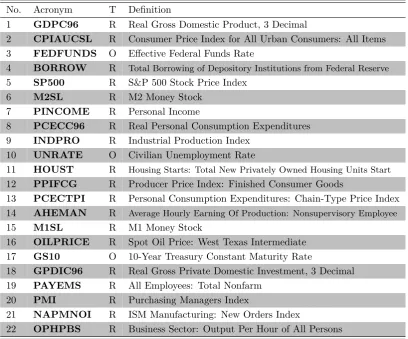
We conduct the estimation for all the competing models in empirical

macroeco-nomics using 22 quarterly series (detailed in Table 2.1) in the US. For each time series,

the data set is composed of 218 discrete time observations from the third quarter of 1958 to the last quarter of 2012, and the first four quarters data are separated as initial

known lags. As indicated in the table, we leave the series, which is already measured as

rates, in its original quantity but transform the others to growth rates using the first diﬀerence of logarithms. We do not transform the series using other methods (e.g.,

[image:34.595.73.482.299.638.2]

second diﬀerence of logarithms) because only univariate models are considered here.

Table 2.1: Variables used in model comparison.

No. Acronym T Definition

1 GDPC96 R Real Gross Domestic Product, 3 Decimal

2 CPIAUCSL R Consumer Price Index for All Urban Consumers: All Items

3 FEDFUNDS O Eﬀective Federal Funds Rate

4 BORROW R Total Borrowing of Depository Institutions from Federal Reserve

5 SP500 R S&P 500 Stock Price Index 6 M2SL R M2 Money Stock

7 PINCOME R Personal Income

8 PCECC96 R Real Personal Consumption Expenditures

9 INDPRO R Industrial Production Index 10 UNRATE O Civilian Unemployment Rate

11 HOUST R Housing Starts: Total New Privately Owned Housing Units Start

12 PPIFCG R Producer Price Index: Finished Consumer Goods

13 PCECTPI R Personal Consumption Expenditures: Chain-Type Price Index 14 AHEMAN R Average Hourly Earning Of Production: Nonsupervisory Employee

15 M1SL R M1 Money Stock

16 OILPRICE R Spot Oil Price: West Texas Intermediate

17 GS10 O 10-Year Treasury Constant Maturity Rate

18 GPDIC96 R Real Gross Private Domestic Investment, 3 Decimal

19 PAYEMS R All Employees: Total Nonfarm

20 PMI R Purchasing Managers Index

21 NAPMNOI R ISM Manufacturing: New Orders Index

22 OPHPBS R Business Sector: Output Per Hour of All Persons

The third column refers to the transformation methods: O = original series, R = growth rate

after the first diﬀerence of logged variables. The sample period (for both O and R transformation methods) was 1958Q3 to 2012Q4. Data were obtained from the St. Louis

FRED database (http://research.stlouisfed.org).

(35)

§2.4 Forecasting Results 17

2 .

4 Forecasting Results

2.4.1 Forecast Evaluation Methods

We divide the data into three sub-samples for a pseudo out-of-sample forecast. The

first part (1958Q3 to 1959Q2) is the separated initial four observations that consider the adopted four lags in the autoregressive models so that all models contain the

same estimation starting point (1959Q3). The second part (1959Q3 to 1974Q4) is the estimation sample, consisting of 62 observations in each macroeconomic variable. The

third part (1975Q1 to 2012Q4) is the hold-out sample, which contains 148 observations.

2.4.1.1 Recursive and Direct Forecasts

The parameters are first estimated from the first data part (say it isy1:T0+t−1) using

MCMC simulation, and they are used to generate the forecasts (ybT0+t+k−1, where kis

k-step-ahead) to be compared with the real data yT0+t+k−1 in the third part. Later

on, we expand the observation window by one more data pointy1:T0+t+1−1, update the

parameters for the next-step discrete time point and forecast again until we consume

the complete data set. In the end, the entire forecast series is obtained by a recursive

computation. For each forecasting loop, the parameter simulation is still based on 50,000 draws with a burn-in period of 5,000.

The expanding windows make the estimation sample part larger, and more infor-mation is used for the newer forecasts. Here we do not use a rolling window, which

keeps the number of estimation samples the same for every forecast, as it does not

like expanding windows that can include more known information with time marching. The expanding windows can also examine whether the forecasting performance of a

candidate model can have less influence from structural breaks in the data.

A direct forecast is conducted in the present chapter rather than an iterated forecast,

since UC group models do not have an iterated formula such as AR group models do. We provide five horizons forecast results, that is, one-, four-, eight-, 12-, and

16-step-ahead forecasts for each of these 22 macroeconomic variables using these 13

specifications. This means that the forecasting results cover from one quarter to four years, so that both shorter horizon and longer horizon performance are investigated

using the proposed specifications.

2.4.1.2 Criteria for Model Selection

To evaluate the quantity of the forecasting performance, two metrics are used: the mean square forecast error (MSFE) and the log-predictive-likelihood (LPL). The MSFE

(36)

a better performance, while the predictive likelihood is used to evaluate the density

forecast performance, where a larger predictive likelihood value implies a better inter-val forecast performance. The MSFE is used widely as a criterion for model selections.

Similar to the variant of an error term, it is a measurement of the magnitude of the

forecasting error (Tsurumi and Wago, 1991). To calculate the MSFE, we first evalu-ate the forecastybT0+t+k−1 by averaging all the posterior meansE(yT0+t+k−1|y1:T0+t)

when it is time T0+t; then the forecasting error is just e2_T₀+t+k−1 = y0T0+t+k−1−

E(yT0+t+k−1|y1:T0+t), where k denotes a k-step-ahead forecast. The next step is to

calculate the mean of the forecasting error. Thus, the MSFE is defined as:

MSFE= 1

T−T0−k+1

T−T∑0−k+1

t=1

e2_T₀₊_t₊_k₋₁

As mentioned in the previous section, an RW model is used as the benchmark. We use

the MSFE values of other models to divide that of the RW model and obtain the relative

MSFE (RelMSFE). Thus, the forecast performance standardizes by setting the perfor-mance of the RW to 1.00. The predictive likelihoodp(byT0+t+k−1 =yT0+t+k−1|y1:T0+t)

is used to evaluate the density forecast performancep(byT0+t+k−1|y1:T0+t), which is the

predictive density of ybT0+t+k−1 evaluated at the observed valueyT0+t+k−1. There is a

close connection between the predictive likelihood and the marginal likelihood. There

is more detailed discussion of the log-predictive likelihood in Geweke and Amisano

(2010). The estimated parameters are conditional on the observed data yT0+t+k−1

producing a larger predictive likelihood value when the observed data fall into the

in-terval of the posterior predictive distribution with higher probability (Hinkley, 1979). The summarized LPL is used here to evaluate the density forecast when considering

easier computation; that is:

LPL=

T−T∑0−k+1

t=1

logp(byT0+t+k−1 =yT0+t+k−1|y1:T0+t)

Since there is no prediction density available for RW, the relative LPL (RelLPL) is

computed using the UC model as the benchmark, and the RelLPL is then obtained using the value of the other models LPL minus that of the UC model. It can be seen

that the RelLPL of UC are all zero and a larger value indicates better prediction density

forecasting for all models except RW.

2.4.2 MSFE Forecast Results

The MSFE and RelMSFE forecast results are tabulated in Appendix 2.B. Here, we

(37)

variables according to diﬀerent errors and diﬀerent model groups, respectively. The

following two tables present the winning times for each specification across short to long horizons, and their winning percentages in the whole data sets are given below

the winning times. Although the results of the MSFE and RelMSFE are kept to four

decimal places, there is still one case where two models, AR2andAR4-MA, tied for the best performance in thek=16horizon for the No. 22 variable forecasting exercise,

so the total number of winning models is 23 and the outperforming percentages are

[image:37.595.146.490.295.496.2]

also calculated by dividing by 23 other than 22.

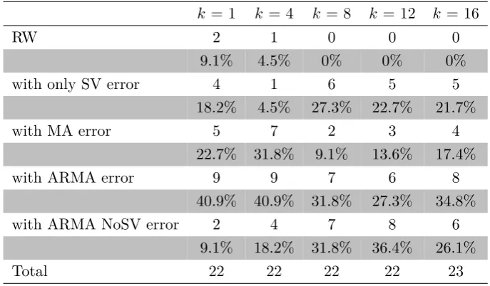
Table 2.2: The number and percentage of the best models with diﬀerent error specifi-cations based on MSFE for 22 macroeconomic variable forecasting.

k= 1 k = 4 k= 8 k= 12 k= 16

RW 2 1 0 0 0

9.1% 4.5% 0% 0% 0%

with only SV error 4 1 6 5 5

18.2% 4.5% 27.3% 22.7% 21.7%

with MA error 5 7 2 3 4

22.7% 31.8% 9.1% 13.6% 17.4%

with ARMA error 9 9 7 6 8

40.9% 40.9% 31.8% 27.3% 34.8%

with ARMA NoSV error 2 4 7 8 6

9.1% 18.2% 31.8% 36.4% 26.1%

Total 22 22 22 22 23

Table 2.2 showsex anteforecasting evidence that models (UC, AR2, and AR4) with ARMA errors yield the best performance for point forecasting prediction in almost all

horizons except Horizon k= 12. For example, in the one-step-ahead forecast, models

with ARMA error have the smallest MSFE for nine variables in comparison with the other models, and this takes up to 40.9%in all 22 variables.

The results also suggest that models with MA error sometimes provide significantly better forecasting results in short horizons (1 and 4), while models with ARMA NoSV

error can give the best predictions in intermediate to long horizons (8 and 12). As

might be expected, even the benchmark RW can win twice in Horizon 1. However, none of these models can present steady good performance over all horizons like the

models with ARMA error. In other words, the results in Table 2.2 support that the

proposed ARMA error term is a robust forecasting device for point forecasts.

We interpret the results in Table 2.3 as important evidence that the UC model is a

(38)

models and the RW model. In Table 2.3, we can see that the UC group models dominate

other models in all horizons except Horizon 4. More specifically, half the variables in longer horizons (Horizons 12 and 16) prefer UC models, and UC models generate more

accurate forecasts than other models for over one-third of variables for a short horizon

[image:38.595.126.431.484.737.2]

(Horizon 1) and an intermediate horizon (Horizon 8).

Table 2.3: The number and percentage of the best models with diﬀerent model group

specifications based on MSFE for 22 macroeconomic variable forecasting.

k= 1 k = 4 k = 8 k= 12 k= 16

RW group 2 1 0 0 0

9.1% 4.5% 0% 0% 0%

UC group 8 7 9 11 11

36.4% 31.8% 40.9% 50.0% 50.0%

AR2 group 7 5 7 4 5

31.8% 22.7% 31.8% 18.2% 22.7%

AR4 group 5 9 6 7 7

22.7% 40.9% 27.3% 31.8% 31.8%

Total 22 22 22 22 23

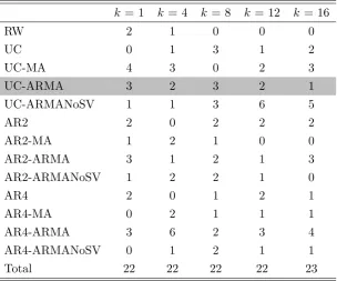
Table 2.4: The number of the best models based on MSFE for 22 macroeconomic

variable forecasting.

k= 1 k= 4 k = 8 k = 12 k = 16

RW 2 1 0 0 0

UC 0 1 3 1 2

UC-MA 4 3 0 2 3

UC-ARMA 3 2 3 2 1

UC-ARMANoSV 1 1 3 6 5

AR2 2 0 2 2 2

AR2-MA 1 2 1 0 0

AR2-ARMA 3 1 2 1 3

AR2-ARMANoSV 1 2 2 1 0

AR4 2 0 1 2 1

AR4-MA 0 2 1 1 1

AR4-ARMA 3 6 2 3 4

(39)

For the two group autoregressive models, the short lag group (AR2) seems to have

better performance over shorter horizons, while the long lag group (AR4) shows better relative performance in longer horizons. It seems that the added lags in AR models

can capture the underlying persistence of the variables in longer horizons but occupy

too much SV in short horizons.

Table 2.4 presents the detailed forecasting performance for each specification. It

is not surprising that no specification can dominate the others for all variables in all

horizons. On one hand, the results in the preceding table suggest that the proposed UC-ARMAcan produces better performance than other specifications for some

vari-ables, such as real gross domestic product in shorter horizons (horizon one and four),

personal income in all horizons except horizon sixteen, real personal consumption ex-penditures in horizon eight, 10-year treasury constant maturity rate in longer horizons

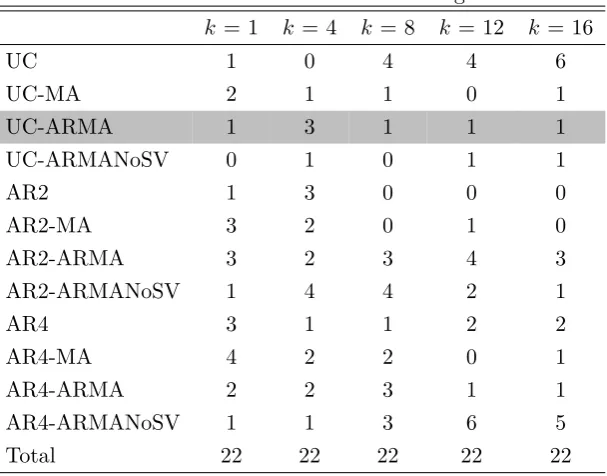
(horizon eight to sixteen), and all employees: total nonfarm in horizon one. On the other hand, UC-ARMANoSV is selected as the best model for many variables in

horizon eight to sixteen, which indicates that UC-ARMA models without SV

specifica-tion can still work well in longer horizons for some variables. Meanwhile,AR4-ARMA is also a highly competitive specifications across forecasting horizons.

2.4.3 LPL Forecast Results

Turning to the analysis of the LPL forecast results in the preceding tables, we can

[image:39.595.145.490.534.708.2]

see that the forecasting performance of all models is slightly diﬀerent from the MSFE results.

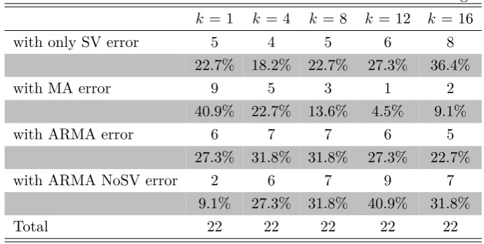
Table 2.5: The number and percentage of the best models with diﬀerent error specifi-cations based on RelLPL for 22 macroeconomic variable forecasting.

k= 1 k = 4 k= 8 k= 12 k= 16

with only SV error 5 4 5 6 8

22.7% 18.2% 22.7% 27.3% 36.4%

with MA error 9 5 3 1 2

40.9% 22.7% 13.6% 4.5% 9.1%

with ARMA error 6 7 7 6 5

27.3% 31.8% 31.8% 27.3% 22.7%

with ARMA NoSV error 2 6 7 9 7

9.1% 27.3% 31.8% 40.9% 31.8%

Total 22 22 22 22 22

(40)

average numbers of best forecasting models in all horizons. The relative performance of

models with only SV and ARMANoSV often improves considerably with longer forecast horizons. These results indicate that a flexible error innovation process may be good at

predicting the short-term evolution of a variable, while long horizon forecasts require

[image:40.595.139.416.250.388.2]

less dynamic specifications in error terms.

Table 2.6: The number and percentage of the best models with diﬀerent model group specifications based on RelLPL for 22 macroeconomic variable forecasting.

k= 1 k = 4 k = 8 k= 12 k= 16

UC group 4 5 6 6 9

18.2% 22.7% 27.3% 27.3% 40.9%

AR2 group 8 11 7 7 4

36.4% 50.0% 31.8% 31.8% 18.2%

AR4 group 10 6 9 9 9

45.5% 27.3% 40.9% 40.9% 40.9%

Total 22 22 22 22 22

Table 2.7: The number of the best model for each specification based on LPL for 22

macroeconomic variable forecasting.

k= 1 k= 4 k = 8 k = 12 k = 16

UC 1 0 4 4 6

UC-MA 2 1 1 0 1

UC-ARMA 1 3 1 1 1

UC-ARMANoSV 0 1 0 1 1

AR2 1 3 0 0 0

AR2-MA 3 2 0 1 0

AR2-ARMA 3 2 3 4 3

AR4 3 1 1 2 2

AR4-MA 4 2 2 0 1

AR4-ARMA 2 2 3 1 1

Total 22 22 22 22 22

In reference to the model group comparison in Table 2.6, the UC group performs

[image:40.595.127.431.451.689.2]

(41)

§2.5 Concluding Remarks and Future Research 23

this time the AR4 group shows a relatively better performance in both the short and

long horizons.

The results in Table 2.7 indicate that each model has its own advantages in

forecast-ing variables with diﬀerent characteristics. Although theUC-ARMAmodel does not

show a significant forecasting performance in interval forecasts, it has its advantages in all the horizons. It provides the best forecasts for real gross domestic product in

horizon four to twelve, personal income in horizon one and four, and real personal

con-sumption expenditures in horizon four and sixteen. It suggests thatUC-ARMAcan forecast some real activity variables well, and it could be helpful in predict the business

cycle for central banks. The ARMA error dynamic introduced in AR2-ARMA also

achieves a substantial forecasting improvement in all the specifications.

The results in the above MSFE and LPL tables suggest that no model or

speci-fication can dominate the others, and the best performing model varies for diﬀerent

variables and forecast horizons. This holds in particular for forecasting metric changes from point forecasts to interval forecasts. When introducing the ARMA error term

into the UC model, the answer as to whether this model can produce out-of-sample forecasts that are better than those from other univariate models seems to be mixed.

Further, the byproductsAR2-ARMAandAR4-ARMAare also highly competitive

models.

2 .

5 Concluding Remarks and Future Research

In this chapter, we have extended the UC model by introducing an ARMA

compo-nent with SV evolution into the error term. By transforming the stacked matrix form of the model, the computation time is significantly reduced, and the serial dependence

induced by the ARMA component is resolved by an eﬃcient precision-based algorithm

developed especially for this model.

This innovation in the error term was tested using 22 macroeconomic variables in the

US data, and the results show that this new component is necessary in estimation and

forecasting exercises for many variables, although not all of them. The point forecasting performance of UC-ARMAdisplays an improvement in forecast accuracy above the

average number of winning models, while the interval forecast results of UC-ARMA show thatUC-ARMAcan produce scores in all forecasting horizons. Future research

(42)

Appendix

2 .A

Full-Sample Estimation Results

Our implementation of an MCMC algorithm and simulation of parameters is straight-forward under a fast precision-based algorithm. The initial values of variables are set

to zero and the prior of parameters are given a mean of zero with large variances. In

total, 50,000 draws are taken and the first 5,000 draws are discarded, so the next 45,000 draws are retained for computing the posterior properties of the interesting parameters.

Posterior Modes of ϕ and ψ

Following Chan (2013) we set the moving average order in the MA-SV model

vari-ants to be one. For consistency, we also set each of the specifications with ARMA(p,q)

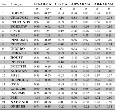
[image:42.595.88.467.379.738.2]

errors to be ARMA(1,1). The results for ϕand ψ of models UC, AR2, and AR4 with ARMA errors, as well as the UC-MA model, are summarized in Table 2.8.

Table 2.8: The modes ofϕand ψin models with ARMA-SVerrors and the mode of

ψin the UC-MAmodel.

No. Acronym UC-ARMA UC-MA AR2-ARMA AR4-ARMA

ϕ ψ ψ ϕ ψ ϕ ψ

1 GDPC96 0.60 -0.17 0.04 0.26 0.03 0.40 0.12 2 CPIAUCSL 0.92 -0.17 0.16 0.83 0.38 0.87 -0.18

3 FEDFUNDS 0.94 0.35 0.99 0.97 0.06 0.96 0.77

4 BORROW 0.99 -0.92 0.05 0.88 -0.99 -0.30 -0.99

5 SP500 0.20 0.20 0.12 -0.34 -0.26 0.31 -0.30 6 M2SL 0.53 0.24 0.41 0.67 0.27 0.95 0.28

7 PINCOME 0.27 -0.19 0.02 0.86 0.07 0.92 -0.05

8 PCECC96 0.43 -0.37 -0.02 0.27 -0.15 0.76 -0.14

9 INDPRO 0.71 0.20 0.38 0.33 -0.31 0.49 0.07 10 UNRATE 0.97 0.99 0.99 0.85 0.14 0.91 0.77

11 HOUST 0.86 -0.33 -0.03 -0.46 -0.99 0.36 0.96

12 PPIFCG 0.35 0.25 0.16 -0.48 0.15 0.59 -0.11

13 PCECTPI 0.89 -0.16 0.11 0.88 0.12 0.76 0.03 14 AHEMAN 0.97 -0.52 -0.15 0.85 -0.48 0.94 -0.05

15 M1SL 0.58 -0.55 0.32 -0.21 -0.05 0.97 -0.17

16 OILPRICE -0.35 -0.18 0.02 0.99 -0.38 -0.53 -0.51

17 GS10 0.89 0.10 0.99 -0.29 0.14 0.95 0.66 18 GPDIC96 0.99 -0.86 -0.04 0.64 0.98 0.39 0.00

19 PAYEMS 0.75 -0.09 0.30 0.56 -0.07 0.80 -0.29

20 PMI -0.99 0.99 0.08 0.56 -0.98 0.72 -0.99

Time-varying Models for Macroeconomic Forecasts