A layered coevolution based attribute boosted reduction using adaptive quantum behavior pso and its consistent segmentation for neonates brain tissue

Abstract—The main challenge of attribute reduction in large data applications is to develop a new algorithm to deal with large, noisy, and uncertain large data linking multiple relevant data sources, structured or unstructured. This paper proposes a new and efficient layered-coevolution-based attribute-boosted reduction algorithm (LCQ-ABR*) using adaptive quantum behavior particle swarm optimization (PSO). First, the quantum rotation angle of an evolutionary particle is updated by a dynamic change of self-adapting step size. Second, a self-adaptive partitioning strategy is employed to group particles into different memeplexes, and the quantum-behavior mechanism with the particles’ states depicted by the wave function cooperates to achieve superior performance in their respective memeplexes. Third, a new layered co-evolutionary model with multi-agent interaction is constructed to decompose a complex attribute set, and it can self-adapt the attribute sizes among different layers and produce the reasonable decompositions by exploiting any interdependency among multiple relevant attribute subsets. Fourth, the decomposed attribute subsets are evolved to compute the positive region and discernibility matrix by using their best quantum particles, and the global optimal reduction set is induced successfully. Finally, extensive comparative experiments are provided to illustrate that LCQ-ABR* has better feasibility and effectiveness of attribute reduction on large-scale and uncertain dataset problems with complex noise, compared with

Manuscript received August 17, 2016; revised February 9, 2017; accepted June 8, 2017 This work was supported by the National Natural Science Foundation of China under Grant 61300167, Natural Science Foundation of Jiangsu Province under Grant BK20151274, Sponsored by Qing Lan Project of Jiangsu Province, Jiangsu Provincial Government Scholarship Program under Grant JS-2016-065, Six Talent Peaks Project of Jiangsu Province under Grant XYDXXJS-048, and Applied Basic Research Program of Nantong under Grant GY12016014.(Corresponding author: Weiping Ding)

W. Ding is with the School of Computer Science and Technology, Nantong University, Nantong 226019, China (e-mail: [email protected]).

C.-T. Lin is with the Computational Intelligence and Brain-Computer Interface (CIBCI) Lab, CAI, University of Technology Sydney, Ultimo NSW 2007, Australia and also with the Institute of Electrical Control Engineering and Brain Research Center, National Chiao Tung University, Hsinchu 30010, Taiwan (e-mail: [email protected]).

M. Prasad is with the School of Software, faculty of Engineering and Information Technology, University of Technology Sydney, Australia (e-mail: [email protected]).

Z. Cao is with the Computational Intelligence and Brain-Computer Interface (CI-BCI) Lab, CAI, University of Technology Sydney, Ultimo NSW 2007, Australia (e-mail: [email protected]).

J. Wang is with College of Computer Science and Technology, Nanjing University of Aeronautics and Astronautics, Nanjing 210016, China (e-mail: [email protected]).

representative algorithms. Moreover, LCQ-ABR* can be successfully applied in the consistent segmentation for neonatal brain 3D-MRI, and the consistent segmentation results further demonstrate its stronger applicability.

Index Terms—Attribute-boosted reduction, adaptive quantum behavior PSO, layered-coevolution with multi-agent interaction, consistent segmentation for neonates brain tissue, sulci and gyrus estimate.

I. INTRODUCTION

ttribute reduction is an important issue that has retained high interest in machine learning, data mining, and pattern recognition. Its aim is to discover a minimal feature subset from a problem domain while retaining high accuracy and efficiency in representing the original data [1]. Rough set theory (RST) is a very efficient and useful mathematical tool that can handle some information and knowledge with uncertainty, imprecision, and vagueness [2] [3]. Introducing RST makes attribute reduction much more popular in modeling and propagating uncertainty and vagueness. When we perform attribute reduction using RST, the main goal is to find the minimum attribute set and induce minimal length decision rules inherent in the information system with affordable algorithmic complexity and computational cost [4][5][6]. So, it usually refers to the preferred technique for data preprocessing in data mining and knowledge discovery [7]-[11].

In recent years, various attribute reduction algorithms and general frameworks for their unification have been discussed. Ke et al. [12] introduced ant colony optimization to the attribute

reduction process to investigate a fast and effective approximation algorithm. This algorithm updated the pheromone trails of the edges connecting each two different attributes of the best-so-far solution, and used a rapid optimization procedure to construct candidate solutions. So, it had the ability to rapidly find solutions with very small cardinality. But this algorithm was unable to effectively deal with large-scale datasets. Yeung et al. [13] proposed the

generalization of fuzzy rough sets, which defined the upper and lower approximation operators by using arbitrary fuzzy relations, and characterized different classes of generalized upper and lower approximation operators of fuzzy sets by different sets of axioms.This generalization was applied to a fuzzy reasoning system, and the results demonstrated it had a wider range of applications. But this model of fuzzy rough sets was sensitive to noisy real-valued attributes. Li et al. [14]

A Layered-Coevolution-Based Attribute-Boosted

Reduction Using Adaptive Quantum Behavior PSO and Its

Consistent Segmentation for Neonates Brain Tissue

Weiping Ding,

Member

,

IEEE

, Chin-Teng Lin,

Fellow, IEEE

, Mukesh Prasad,

Member

,

IEEE

,

Zehong Cao, and Jiandong Wang

proposed a neighborhood based decision- theoretic rough set model in which the positive region related attribute reduction and its minimum cost were analyzed. This model can overcome the shortcomings of the current decision-theoretic rough set model and obtain a short reduction set with competitive classification ability. Qian et al. [15] exploited a new

framework structure to speed up the computation of equivalence classes and attribute significance by parallelizing the traditional attribute reduction process based on the MapReduce mechanism. This parallel attribute reduction algorithm performed efficiently on massive data. So, the paradigm with the MapReduce technique had good feasibility to facilitate big datasets. Maji et al. [16] put forward the IT2

fuzzy-rough set-based attribute selection method, where the lower and upper relevance and significance of attributes were defined for IT2 fuzzy approximation spaces, and then attributes were selected by maximizing the relevance and significance. This method had the good utility effectiveness for fuzzy attribute reduction. Real-world datasets are now available everywhere from the Web, sensor networks, social networks, and proprietary databases, which often link multiple relevant data sources, structured or unstructured. Moreover, the scale of datasets increases dynamically with time variation. So, an abundance of staggeringly complex large datasets has been produced [17] [18]. Most of the above-mentioned algorithms are inadequate and unreliable for attribute reduction for these datasets due to their ever-greater volume, complexity and diversity of structures. Besides, noise is one of the main sources of uncertainty in applications, and it has also been shown that traditional attribute reduction operators are not robust to noise. Hence, there is an urgent need for new and effective attribute reduction algorithms to remove irrelevant and redundant datasets while retaining the optimum salience in these complex large-scale datasets.

In the past few years, the quantum-inspired evolutionary algorithm (QEA) has attracted significant attention from researchers by using a Q-bit as the probabilistic representation, without numeric or symbolic representation. This appears to be a much better characterization of population diversity, and thus this representation has the strong advantage of denoting the linear superposition of evolutionary states [19]. It has been empirically and theoretically demonstrated that QEA always gains better performance than the traditional evolutionary algorithm (EA) [20][21][22]. We know that the implementation of attribute reduction algorithms on large and complex datasets is very time-consuming due to the dramatic increases in the number of attributes because of complex, fast-changing relationships between big data objects. Therefore, to propose an effective and efficient attribute reduction algorithm based on the superiority of QEA becomes a significant and urgent challenge. Some work is required to solve this problem. First, some effective quantum-inspired evolutionary operators and mechanisms are designed to enhance attribute reduction of datasets with high-dimension. Second, the interacting decision variables among various attribute sets can be handled well to achieve better performance in practical applications. In addition, some limitations of existing co-evolution structures can be addressed to decompose large-scale attribute sets by using the dynamic adaptation of a reorganization model.

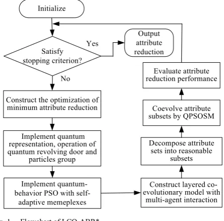
This study proposes a new and efficient layered- coevolution-based attribute-boosted reduction algorithm (LCQ-ABR*) using quantum behavior PSO. It aims to choose attribute subsets including strongly relevant and non-redundant attributes for large-scale, noisy, and uncertain datasets linking multiple relevant data sources. The main flowchart of LCQ-ABR* is shown in Fig. 1. Its performance is extensively evaluated to solve large-scale and uncertain dataset problems with complex noise on some well-known benchmark datasets. The experimental results illustrate that LCQ-ABR* has better feasibility and effectiveness than some representative algorithms to which it is compared. Moreover, LCQ-ABR* is applied to the consistent segmentation for neonatal brain 3D-MRI, and it can achieve better feasibility and effectiveness in complex neonatal brain tissue.

Output attribute reduction Initialize

Satisfy stopping criterion?

No Yes

Construct the optimization of minimum attribute reduction

Implement quantum-behavior PSO with

self-adaptive memeplexes

Decompose attribute sets into reasonable

subsets Coevolve attribute subsets by QPSOSM

Construct layered co-evolutionary model with

multi-agent interaction Evaluate attribute reduction performance

Implement quantum representation, operation of quantum revolving door and

particles group

Fig. 1. Flowchart of LCQ-ABR*

We briefly state key contributions of the work presented in this paper below.

1) The quantum rotation angle of evolutionary particles can be updated by the dynamic change of the self-adapting step size. A new self-adaptive partitioning strategy is employed to group particles into memeplexes, and the quantum- behavior mechanism of particles cooperates better in their respective memeplexes to achieve superior performance. These new quantum operators aim to strengthen the adaptive stability of particle memeplexes for attribute reduction in large-scale datasets.

2) A new layered co-evolutionary model with multi-agent interaction is constructed to decompose attribute sets, and it can self-adapt the attribute sizes among different layers and produce reasonable decompositions by neighborhood vectors among multiple relevant attribute subsets. It adapts the dynamic stability of co-evolutionary particle behavior to achieve a complementary cumulative distribution. So, it boosts the optimal performance of attribute reduction. 3) LCQ-ABR* is applied to the longitudinal cortical surface

[image:2.595.312.538.256.478.2]

expected to dramatically scale up attribute reduction algorithms for large-scale datasets in terms of efficiency and feasibility.

This paper is organized as follows. First, the optimization model of minimum attribute reduction is constructed in section II. Section III introduces the quantum-behavior PSO with self-adaptive memeplexes (QPSOSM), which illustrates the quantum rotation angle, self-adaptive partitioning memeplexes strategy and quantum-behavior mechanism of particles. A layered co-evolutionary model with multi-agent interaction (LCMMI) for attribute reduction is presented in section IV. In section V, the main steps of LCQ-ABR* are stated in detail. Extensive experimental evaluation and discussion are provided in section VI. In section VII, the application performances of LCQ-ABR* are assessed in the consistent segmentation for neonates brain tissue 3D-MRI. Section VIII presents some discussions of experimental results. Section IX provides the conclusion.

II. OPTIMIZATION MODEL OF MINIMUM ATTRIBUTE REDUCTION

The approximation space

K



( , )

U R

is characterized by

using an information system

S



( , , , )

U A V f

, where

U

_is

the non-empty finite set of objects,

A

is the non-empty finite set of attributes,

V

is equal to

a a A V



(

V

_a is the domain of attribute

a

), and

f

is an information function

U A

 

V

such that f x a( , )Va for each

x U a



,



A

.

Definition 1: For any concept

X



U

and attribute subset

R



A

, X can be approximated by the R-lower approximation

RX

and R-upper approximation

RX

, with

RX



{

x



U

| [ ]

x

R



X

}

(1)

and

RX



{

x



U

| [ ]

x

R



X

 

}.

(2)

RX

is the set of objects of

U

that will surely belong to

X

, whereas

RX

is the set of objects of

U

that can possibly belong to

X

.

[image:3.595.305.547.83.341.2]

Definition 2 : When

C

is a set of condition attributes,

D

is a set of decisions, and

A



C



D

(

C



D

 

), the information system

S



( , , , )

U A V f

is called a decision

table. The

C

-positive region of

D

is the set of all objects from the universe

U

that can be classified with certainty into classes of

( / )

U D

employing attributes from C, that is

/

( )

.

C

X U D

POS

D

CX





_

(3)

The criterion for attribute reduction is the degree of dependency



C( )Q , which is defined as

( )

( )

|

|

C C

POS

Q

k

Q

U







_{. (4)}

Definition 3: For attribute reduction, a reduction is defined as a

subset

R

of conditional attribute set

C

_{that is satisfied with}

( )

( )

R

D

C

D







. The reduction set is given by

{

|

( )

( ),

,

( )

( )}. (5)

R C

B C

RED

R

C

D

D

B

R

D

D















 



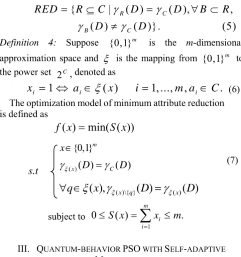
Definition 4: Suppose {0,1}m _{is the m-dimensional}

approximation space and



is the mapping from {0,1}m _to

the power set ₂C_{, denoted as}

1

( )

1,..., ,

.

i i i

x

 

a





x

i



m a



C

(6)

The optimization model of minimum attribute reduction is defined as

( ) min( ( ))

f x



S x

(7)

subject to

1

0

( )

m i

.

i

S x

x

m











III. QUANTUM-BEHAVIOR PSO WITH SELF-ADAPTIVE MEMEPLEXES

In this section, we propose the quantum-behavior PSO with self-adaptive memeplexes (QPSOSM) for attribute-boosted reduction. Assume that the PSO evolutionary system is a quantum system and each evolutionary individual is described by a particle in the quantum space. Then, the rationales for using this hybrid combination of PSO and quantum technology are as follows.

First, evolutionary particles are represented by multi-state quantum bits, which represent a linear superposition of states in the particle search space probabilistically, in order to increase the diversity of evolutionary particles.

Second, the adaptive updating strategy of the quantum rotation angle is adopted to update the operation of a quantum revolving door. This strategy speeds the search process for evolutionary particles in different memeplexes, so that they can keep the balance between global search and local refinement during attribute reduction.

Third, a self-adaptive partitioning strategy is employed to group particles into different memeplexes, and the state of a particle is represented as the wave function, instead of position and velocity in standard PSO. Each particle moves with the potential in each dimension through the establishment of a delta trap, which will greatly accelerate the evolution convergence. Two abilities of exploration and exploitation are well balanced to achieve better performance at attribute reduction.

A. Adaptive Updating Strategy of Quantum Rotation Angle

QPSOSM uses a new representation of a quantum bit (Q-bit), whereone Q-bit is denoted as a pair of complex numbers

( , )

 

_{such as}

|



 



| 0

 



|1 ,



(8)

where



and



are complex numbers that specify the probability amplitudes of corresponding states. The quantities

{0,1}m x

( )x ( )D C( )D









( )\{ } ( )

( ),

_{x q}

( )

_x

( )

q



x



_

D



_

D

 



2

| | and |



|2give the probabilities that the Q-bit is found in the “0” or “1” state, respectively. The normalization condition of their states to unity guarantees that

2 2

| |





|



|



1.

(9)

The quantum gate (Q-gate) is used for the rotation gate according to the relationship

cos( ) -sin( )

( )

.

sin( ) cos( )

i i

i i

U















 







(10)

The ith Q-bit is updated as shown such that

cos( ) -sin( )

( )

,

sin( ) cos( )

i i i i i

i i i i

i

U

























_

_



_{ }

_







(11)

where



i is the rotation angle toward either the “0” or “1”

state, depending on its objective sign.

For a decision variable

x



( , ,..., )

x x

1 2

x

n , where

[

,

],

1, 2,...,

i

x



lower upper i



n

, the quantum rotation angle is updated by the adaptive strategy as follows:

Algorithm 1: Adaptive updating strategy of quantum rotation angle

1) Each

x

iis mapped into [0,1] according to the following

equation

  , 1, 2,...,

 i i

x lower

x i n

upper lower . (12)

2) Implement the quantum real coding to get x as

1 2

2 2 2

1 2

...

1 ( ) 1 ( ) ... 1 ( )

 

  _ _

  

 

n

n

x x x

x

x x x . (13)

3) For some Q-bit i of x, compute the rotation angle

( , )

d i j

 

 

,rand(0.6, 0.9), where

d i j

( , )

is the random rotation direction. t

(

1, 2,..., )

j

p

j



n

is the

state of the tth iteration, defined as

1 2 1 2

11 12 21 22

11 12 1 21 22 2 1 2

...

...

...

...

...

...

...

...



_

 

_

_





t t t t t

t t t t

l l m m ml

t

j _{t t t t t t t t t}

l l m m ml

p

 



 



 



 

  



 



. (14) 4) Get

x

i



as

2

sin( ) cos( ) 1 ( ) .

     

i i i

x



x



x (15)

5) Update





2     i i i

x x

x _{if the Q-bit is out of [0, 1].}

6) Repeat above operation until each Q-bit is within [0, 1].

B. New Strategy for Partitioning Particles into Self-adaptive Memeplexes

The proposed kernel strategy for partitioning particles combines the geometric partitioning method and the memeplexes model that is used to represent “networks of particles.” Particles cooperate better in their respective memeplexes and achieve superior performance. The

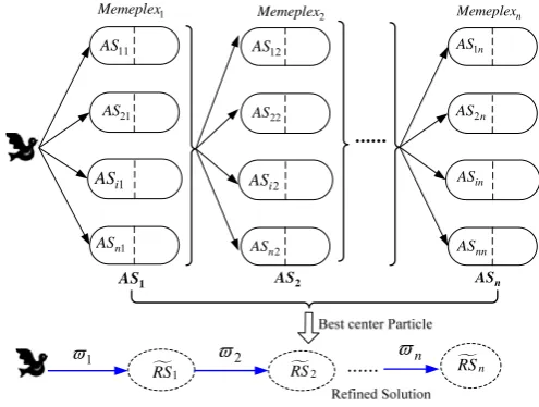
partitioning method aims to group particles in one vicinity in the same memeplex. First, the center position of each memeplex is selected randomly, and then the particles are grouped according to their geometric distance from the best center particle of each memeplex, as illustrated in Fig. 2. To better represent the attribute reduction solutions, the particles in each partitioned memeplex are used to optimize their corresponding attribute variables. Fig. 3 shows the graphical procedure of the refined attribute reduction solution. Each memeplex is assigned n attribute variables representing the n candidate solutions. The main steps are as follows.

Search Space

Memeplex2 Memeplex1

Memeplexi Memeplexn

Best center Particle1

Best center Particle2

Best center Particlei

Best center Particlen

Particles of Memeplex1

Particles of Memeplex2

Particles of Memeplexi

Particles of Memeplexn

…

…

…

…

Fig. 2. Schematic diagram for partitioning particles into memeplexes

11 AS

21

AS

1 i

AS

1

n

AS



1



₁

RS RS2 RSn

1

Memeplex

AS2 ASn

12 AS

22

AS

2 i AS

2

n AS

1n AS

2n AS

in AS

nn

AS

AS1

2

Memeplex Memeplexn

2

 n

     

Fig. 3. Graphical representation of refined attribute reduction solution Algorithm 2: Self-adaptive memeplex of partitioning

particles for attribute reduction

1) Create evolutionary particles, initialize them in the quantum population space, and construct the memeplex of partitioning particles as follows. First, calculate the distance between center position 1 and all other particles, denoted as

l1. If the particles have less distance than l1, they are assigned to Memeplex1. Second, calculate the distance between center position 2 and all remaining particles, denoted as l2. If the particles have less distance than l2, they are assigned to the Memeplex2. Continue this process until all particles are assigned to Memeplex3,…, Memeplexn, respectively.

[image:4.595.313.551.213.368.2] [image:4.595.303.551.396.583.2]

the respective n memeplexes as the center position of their

corresponding memeplexes.

3) Along with the particles’ partitioning, if the local best fitness of most memeplexes reaches the same target area, the result is nearly the same even though the particles learn from any memeplex. If we continue to partition particles, the consumption will be increased. So, we will merge the relevant memeplexes into a new memeplex according to the diversity value of the local best fitness of memeplexes. Diversity is computed as

1 ( )

( )

diversity t cn t

 , (16)

where cn t( ) represents the sum of the difference numbers in each dimension that meet the threshold set 

between the local best fitness of the memeplex in the tth

iteration and the average fitness from the 1st _{to the (}

t-1)th

iteration. It can be defined as 1

1

( ) n ( k( ))

k

cn t f lbest t









(17a)

1, ( ) ( )

( ( ))

0, .

kj j

k

j lbest t lbest t f lbest t

otherwise 

 _{  }

  

 (17b)

1 1

( )

( ) ,

1 n

kj k j

lbest t lbest t

n 

 





(17c) where t1, 2,...,n, lbest t_j( ) represents the average fitness from the 1st _{to the (}

t-1)th iteration.

If diversity t( ) 1/[ ( c n1)], _where c _{is a uniform}

random number and

c



[0,1]

, the relevant

memeplexes will be merged.

4) A particle path starts from the nest (denoted as variable

11

AS ), passes through nodes for variables AS₁₂,...,AS_1(n1),

and stops at a node for variable ₁

n

AS . A particle path

includes n edges, and each edge will construct a solution

component in the solution vectorAS_i.

5) The credit assignment for partitioning particles is performed at the memeplexes. It is computed by estimating how well the best center particle in the ith

memeplex performs relative to its competitors in cooperating with other particles. In the ith memeplex, the

best center particle is assigned credit



_i based on the equation





i i

i

CP Mem i

CP

f

f

f



, (18)

where

i

CP

f

is the fitness of the ith best center particle and

i

Mem

f

is the average local best fitness of the ith

memeplex.

6) Set memeplex i for representing attribute subset i, and

best particle i for representing attribute i. For j=1 to the ith

memeplex

|

S

i

|

do

(a) Assemble the complete solution with

S

_ij (the jth

particle of

S

_i) and representative from the other memeplexes;

(b) Assign Pareto rank to

AS

_ij; (c) Calculate the niche count of

S

_ij;

(d) Update the best center particle of AS_i.

7) Assigned a credit



_i to the best center particle of ASi,

and update the archive of the nondominated solution vectors as follows:

₁

1 1

  

RS AS ; RS2  2 AS2; …



i

  

i i

RS

AS

; …



RS

n

  

_n

AS

_n.

So,



1

(

)

n

i i

i



_

 

AS

RS

.

8) Check elimination criterion if the maximum iteration number has reached the termination condition, otherwise continue with Step 5.

Using the proposed strategy of partitioning particles, each memeplex has a vicinity filled by particles within a close distance of each other, with credit assigned for the best center particle. It can provide a way of complementing the diversity preservation, and can produce more diverse particles across the different memeplexes in the quantum space.

C. Quantum-Behavior Mechanism of QPSOSM

QPSOSM adopts a new quantum-behavior mechanism to guarantee the global convergence of PSO. The state of a particle in the quantum space is represented by the wave function



( , )

x t

, and each particle moves with  potential in each dimension through the establishment of a delta trap. By this wave function



( , )

x t

, the particle’s position of a wave function and its probability density function are achieved. So, the quantum-behavior searching mechanism is deduced, and its steps are described as follows:

Algorithm 3:Quantum-behavior mechanism of QPSOSM

1) At the number of iterations

t

, the th

i

particle in the

j

th

dimension quantum space has the attractor t ij

p

. The wave function at iteration t+1 can be expressed as

)

/H

|

|

exp(

1

)

(

1 t

ij t ij t ij t

ij t

ij

x

p

x













, (19)

where t ij

 is the standard deviation of the double exponential distribution, and it will change with the number of iterations t.

2) Construct the Lévy flight model for quantum-behavior particles in the quantum space as

α β( , , )exp  (1 ( ))













,

k

k i k k i k,

k



is the displacement,  is the measure,



is the characteristic exponent,



is the skewness, and we set

= 0.5, = 1



.

3) The probability density function with double exponential distribution

Q

is

1 2 1

( t ) ( ) | ( ) |t ( ) exp( 2 | t t | /H )t

ij ij t ij ij ij

ij

Q x L vy  x L vy   x p 

 

é é

(21)

where L vyé ( )



denotes the random search vector of theL vyé distribution with parameters



(1



3).

4) Compute the corresponding probability distribution function as

(

)

1

exp(

2

|

|

/H

).

1 t

ij t ij t ij t

ij

x

p

x

F











(22)

5) Implement the strategy of self-adapting step size



as follows:

max max

1 1

1

_,

1

_,

g g

g g

U k b

b



 

 









_





_





(23)

where U (. , .) is a uniform random number, k is the number of particles in each memeplex, g is the current

iteration number, and gmaxis the total number of iterations.

The parameter



can adjust the step size dynamically near the better solutions and enhance the searching ability of particles as follows:

(a) When g is quite small,



is very large and the

operation can achieve a comprehensive fast global search. The searching range of global search is [0, k];

(b) When g gradually increases to gmax,



can

self-adaptively reduce to a small value and the improvement of local searching ability can be realized by reducing the step size. The range of the local search is [0, b].

6) Obtain particle

x

_i in the

j

thdimension quantum space and the (t+1)th iteration, and update its position as

follows:

1 1 _{ln(1/ )}

2

t t t t

ij ij ij ij

x p 



  u ,

(24a)

| |

2 t

ij t j t

ij c x





, (24b)

where t ij

u

is a uniformly distributed random number in (0,1), the parameter



_{is set as}  1.782 to guarantee convergence of the particle in each memeplex, and



can be controlled to decrease linearly from



₀ to



₁, where

 

0

,

1

(



0





1

)

are two uniformly distributed random numbers that can be selected from the range [0.7,1.5], and the values of

 

0

,

1 express the degree of relative importance of particle

x

_i and self-adapting step size



in the updating process.

7) Design the global point of the particle population in the quantum space, denoted as C , which is defined as the average position of the best center particle among each

memeplex. Its equation is

1 1 1 2

1 1 1

1

1

1

( , ,..., )

t t t M t

,

M t

,...,

M t

,

j i i ij

i i i

C

c c

c

x

x

x

M



M



M









_{ }

_











(25)

where M is the number of updated memeplexes and t ij

x

is the best position of particle i in the

j

thdimension quantum

space at the (t+1)th iteration.

By the above-mentioned QPSOSM, the quantum rotation angle of evolutionary particle dimension in the quantum space is updated by the dynamic change of the self-adapting step size, and the quantum-behavior mechanism with the particles’ states depicted by the wave function cooperates to achieve superior performance in their respective memeplexes. Hence, QPSOSM will strengthen the adaptive stability of particle memeplexes for attribute reduction in large-scale datasets.

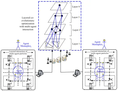
IV. LAYERED CO-EVOLUTIONARY MODEL WITH MULTI-AGENT INTERACTION FOR ATTRIBUTE REDUCTION To solve the optimization problem of large-scale attribute reduction, a layered co-evolutionary model with multi-agent interaction (LCMMI) is constructed to adaptively partition the multiple-relevance attribute sets into different subsets by avoiding dependency on prior domain knowledge. The model can keep the interdependencies of multiple relevance attribute sets to a minimum to achieve a dynamical balance between exploring and exploiting inherent structures of attribute sets.

Each agent corresponds to a neighborhood vector with different resolutions, and can capture the multiple-relevance attribute decision variables and group them together in one memeplex. It allows a better approximation of the contribution of various neighborhood vectors, uncovers the underlying interaction structure of attribute decision variables, and optimizes attribute-boosted reduction.

This LCNRH constructs a hierarchical framework of neighborhood vectors for partitioning an attribute set as described in Fig. 4. The main steps are as follows:

First, according to factor h of the partition, each agent is

divided into such parts as “Head (h)” and “Tail (t)=(n-1)*h+1”.

Thus, the attribute in each layer is divided into m agents.

Second, to map an attribute set into different layers, the computation of neighborhood vector interactions is initially conducted on Layer1, and then propagated to other layers effectively via the distribution neighborhood vector that indicates the relationship of neighborhood vectors from Layer2, Layer3, and Layer4.

Third, generate four interaction neighborhood vectors in 4

L _as R4_p, R4_t , R4_n, and R4_m, and decompose R4_p, R4_t , 4

n

R , and R4_m into four vector subsets as 4 _[ 1_, 2_, 3_, 4 T_]

p  Rp Rp Rp Rp

R ,R4_t [ ,R R R R_t1 _t2, _t3, _t4 T] , 4 _{[ ,}1 2_, 3_, 4 T_]

n  R R R Rn n n n

R ,R_m4 [R_m1,R_m2,R3_m,R_m4 T] . (26)

cascade between layers are considered not only for attribute reduction with the same scale in the same layer, but for attribute reduction across different scales in different layers as well. So, this strategy ensures that the underlying similarity of

information between any pair of neighborhood vectors in the same layer can be fully reflected and results in better generalization ability. Its detailed investigation is included as follows.

Layered interactionof multi-agent particles

1

t

R 4

t

R

…

1

p

R 4

p

R

…

4

p

R 4

m

R

4

n

R 4

m R

…₁

m

R

4

n

R

…₁

n

R

4

t

R

Layered interactionof multi-agent particles

1

t

R 4

t

R

…

1

p

R 4

p

R

…

4

p

R 4

m

R

4

n

R 4

m R

…₁

m

R

4

n

R

…₁

n

R

4

t

R

Layer 1 Layer 2 Layer 3 Layer 4

Layered co-evolutionary optimization with multi-agent

interaction

Agent

Memeplexj

Agent

Particlej

Agent

Particlei

Agent

Memeplexi

Fig. 4. Hierarchy framework of neighborhood vector for partitioning attribute set

Fig. 5. Layered co-evolutionary optimization with multi-agent interaction

(2) Map attribute set

Layer 1 Layer 2 Layer 3 Layer 4

(3) Optimize attribute vector (1) Construct multi-agent chromosome

Head

t=(n-1)*h+1 h

Tail

agent1 agent2 ... agentm

Single agent with head and tail part

Multi-agent chromosome consisted of m agents

4 m

R

4

t R

4 p

R

4 n

[image:7.595.67.522.145.327.2] [image:7.595.95.491.359.662.2]

Algorithm 4. Layered co-evolutionary optimization with multi-agent interaction

1) Construct the four-layers structure based on the self-organizing neighborhood vector, in which the ith layer

corresponds to the efficient solution of the ith

neighborhood vector _Ri

.

2) Obtain the N4N4 matrix as C4, where N is the

number of neighborhood vectors in Layer4. The Pearson correlation between attribute vectors f_i and f_j is

4 4 , 1

( , ),







_{i j} i j

corr

C f f

(27)

where f_i ,f_jdenote the volumetric ratios of attribute vectors of the ith and jth neighborhood vector in Layer4,

respectively.

3) Construct the membership decomposition matrix i M _,

which includes i rows and N4 columns. Each row

corresponds to the simple neighborhood and each column corresponds to the single neighborhood in Layer1. 4) Calculate the interaction margin value of any two

interaction neighborhood vectors in Layer4 as

4 4 4 4

4 4 1 4 4

( , ) ( , ),

 





 

m m t t

t m t m

corr corr

a b_{R S R S}

R R R R (28)

where 4

t

R and R4_m represent the attribute neighborhood vector in Layer4, including a and b neighborhood vectors,

respectively. 4

t

S and S4_m are two simple neighborhood sets that comprise 4

t

R and R4m, respectively.

5) Compute the cross energy between the Agent_Memeplexi

and Agent_Particlej as













Agent_Memeplex Agent_Particle =1 Agent_Memeplex Agent_Particle =1 Energy Agent_Memeplex 1

= 0.6 same ,

2*

+1.4 same ,

i j i j i n j n k x x n f f       _ 





(29a)

where _{Agent_Memeplex} i

x

is the best position of

Agent_Memeplexi ,

x

Agent_Particle_j is the best position of Agent_Particlej,

f

Agent_Memeplexi is the best fitness of Agent_Memeplexi, and

f

Agent_Particle_j is the best fitness of Agent_Particlej. The function same( ) is calculated as

 

0,

same ,

1, .

x = y x y otherwise     (29b)

6) Construct the energy proximity matrix EPM of multi-

agent interaction as

2

1 1 1

1

2 2 2

1 2 π π π π π π n n

n n n

En En En       _{ }       EPM        _, (30)

where En_i=Energy Agent_Memeplex

_

_i

_

and

Agent_Memeplex Agent_Particle

π = i

j

j i

f

f .

7) Achieve the ensemble set of neighborhood vectors in the ith

layer as 1 ,      _     _  



N i i i i i

t p n m

i

En

R R R R

EPM

(31)

where the symbol



denotes the vector matrix product.

V. PROPOSED LCQ-ABR*ALGORITHM

Based on the above-mentioned quantum-behavior PSO with self-adaptive memeplexes (QPSOSM) and layered co-evolutionary model with multi-agent interaction (LCMMI), this paper proposes a new and efficient layered-coevolution- based attribute-boosted reduction algorithm (LCQ-ABR*) using adaptive quantum behavior PSO. The decomposed attribute subsets are co-evolved by their best quantum particles with QPSOSM, respectively. The optimal reduction subset of each attribute subset can be easily obtained, and then the global optimal reduction set is also induced successfully. Its main steps are as follows:

Algorithm 5: LCQ-ABR*

1) Set up a searching space of m dimensions for the

attribute reduction in the quantum space, and construct the co-evolutionary memeplexes, in which each memeplex represents its corresponding attribute subset. 2) Partition particles into different memeplexes using

Algorithm 2, and map each memeplex into one condition attribute subset that is limited to the defined space of attribute reduction by

min max i i i Weight Weight Weight Weight Weight  

 . (32)

3) Construct the optimization object of minimum attribute reduction as F x( )min S x( ( )).

4) Calculate the lower ( )

i

A D

 and upper ( )

i

A D

 relevance

of each attribute A_iC, and then select out the most

relevant attribute A_i with the highest lower relevance value ( )

i

A D

 .

5) Generate a quantum particle chromosome by giving 2

| | and _{| |} 2 _{in each Q-bit individual. Encode the} quantum evolutionary particle’s position as the subset of condition attribute set C.

6) Make quantum particle states Q t( ), where the observation individuals corresponding to the ith Q-bit particle are

represented by ( 1, 2,..., )

t t t

i i in

X X X .

7) Update Q t( ) to Q t( 1) by using the adaptive updating

strategy of quantum rotation angle in Algorithm 1. Conduct the proposed quantum-behavior mechanism for best center particles in the memeplexes by using Algorithm 3.

by using Algorithm 4. Both within- and between-layer neighborhood vector interactions are performed to achieve the ensemble set of neighborhood vectors. 9) Do {

(a) Select attribute subsets

(

Sub attribute

_

)

iwith

parallel model;

(b) Calculate the lower significance of

A

j (

A

j



C

)

with respect to each selected attribute

A

_i



S

by

_{{ , }}

{ , }

( , )

( )

( )

i j _{i j i}

A A

D A

j _{A A}

D

_A

D











;

(c) Calculate the degree of dependency



R

( )

D

as

comparison criterion for attribute reduction; (d) Remove

A

j from

C

if _{{ , }}( , ) 0

i j

A A D Aj

  for any

attribute

A

_i



S

;

(e) From the remaining attributes of

C

, repeat similar

steps of the upper significance until the desired number of attributes is selected out or

C

 

;

(f) Calculate the fitness Fit x( ), and select out the local

best reduction subset in every memeplex; (g) Achieve the minimal solution of reduction subset

best i

R

.

} While (the stopping criterion is satisfied).

10) Evaluate whether attribute reduction accuracy is satisfied with the stopping criterion.

If satisfied, Output the entire minimum attribute reduction

1 n

best

Emin i

i

RED R

 

_

.

Otherwise, Go to Step 7 and continue to implement the attribute reduction procedures.

VI. EXPERIMENTAL STUDIES

The objective of the following experiments is to show the effectiveness and efficiency of LCQ-ABR* compared with traditional algorithms. To support data-intensive distributed applications, our experiments run on the open platform Apache Hadoop. We implement all algorithms on a cluster with ten nodes, and each node is provided with 128 GB main memory and an AMD Opteron Processor 2376 with 2 Quad-Core CPUs. For distributed experiments of large-scale datasets, one is configured as the master node and the rest are set as slave nodes. The operating system in these machines uses Linux CentOS 6.5 Kernel 3.18. We have chosen 16 benchmark datasets whose characteristics are summarized in Table 1. There are three protein datasets (Pancreatic, Colorectal and LiverACO), two metabolism datasets (LiverM and LiverTOD), four NIPS 2003 feature selection challenge datasets (Arcene, Dexter, Dorothea, and Madelon), four public microarray datasets (Colon, Prostate, Leukemia, and Lung-cancer), and three biomedical data- sets (Breast-cancer, Ovarian-cancer, and Hiva). These 16 benchmark datasets cover a wide range of real-world application domains, including protein, metabolism clinical image, gene expression, ecology, text categorization, and molecular biology; sample sizes (from 62 to 4,229); and features (from 115 to 100,000). Hence, they are significant

challenges to the construction and reduction of attribute sets by using some attribute reduction algorithms. For the four NIPS 2003 challenge datasets, we employ the originally provided training sets and validation sets; for four public microarray datasets, we randomly adopt the first 3/5 samples for training and the last 2/5 for testing; and for the rest we take ten-fold cross-validation. The software used is Microsoft Visual Studio 2015 and Visual C# 6.0. For the following results, we present the average testing values of 30 runs.

TABLE I

CHARACTERISTICS OF 16 BENCHMARK DATASETS

Dataset #Sample #Feature Dataset #Sample #Feature

1. Pancreatic 181 664 9. Madelon 2,000 500

2. Colorectal 112 779 10. Colon 62 2,000

3. LiverACO 975 129 11. Prostate 102 6,033

4. LiverM 126 115 12. Leukemia 72 7,129

5. LiverTOD 280 866 13. Lung

-cancer 181 12,533

6. Arcene 100 10,000 14.Breast

-cancer 286 17,816

7. Dexter 300 20,000 15.Ovarian

-cancer 216 2,190

8. Dorothea 800 100,000 16. Hiva 4,229 1,617

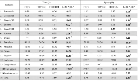
In this experiment, the attribute reduction performance of the proposed LCQ-ABR* algorithm is conducted to compare with such representative algorithms as FRFS [5], FRRFDM [9], and TDNEC [14]. Table 2 summarizes the comparative results of reduction running time (Time) and space consumption (Space) for FRFS, TDNEC, FRRFDM, and LCQ-ABR*, respectively. The superscript symbol “†” means that the corresponding result is significantly best, “－” indicates no trial can reach an acceptable solution, and bold indicates that the mean value is greater than those of the other three algorithms.

As described in Table 2, LCQ-ABR* typically shows the highest reduction speed, compared with FRFS, TDNEC, and FRRFDM. For the Arcene dataset, the reduction time by LCQ-ABR* is 3.76 s, while the reduction times by FRFS, TDNEC, and FRRFDM are 7.78 s, 6.54 s, and 6.08 s, respectively. LCQ-ABR* can significantly improve the reduction running time. In addition, LCQ-ABR* needs lower space consumption. For example, LCQ-ABR* spends 54.06% space consumption in the Dorothea dataset and 73.09% in the Breast-cancer dataset of FRRFDM. Similar results are evident in most datasets. Therefore, the experimental results indicate that, LCQ-ABR* can find a feasible attribute reduction subset in much less time and space, compared with FRFS, TDNEC, and FRRFDM.

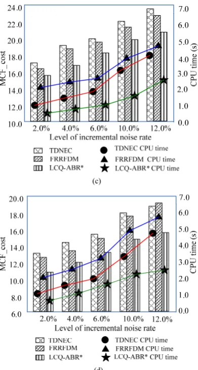
Moreover, we observe the variation of average misclassification cost on four kinds of datasets (Pancreatic, Dorothea, Leukemia, and Breast-cancer) with an added attribute noise rate. We assume n_{NI is the number of objects} classified incorrectly, n_{ND is the number of objects with} deferment decisions,



CP is the cost for classifying an object

[image:10.595.81.536.503.769.2]

MCF_costn_ND



_CPn_NI



_{CP. (33)} Fig. 6 presents the average comparison results of misclassification cost and its corresponding running time of attribute reduction. The x-axis contains different levels

(2.0%~12.0%) of incremental noise rate, and the y-axis shows

the variation of updating misclassification cost (MCF_cost) and CPU time. We can observe the variation of MCF_cost and CPU time of three algorithms as the level of noise rate increases. This indicates that the noise has a great effect on the MCF_cost performance. But we can see from Fig. 6 that the value variation of LCQ-ABR* is small in most cases. Taking the Dorothea dataset (one of the NIPS 2003 feature selection challenge datasets) as an example, when the level of noise rate is from 8.0% to 10.0%, the variation of MCF_cost of LCQ-ABR* is 1.98. And when the level of noise rate is from 10.0% to 12.0%, the variation of MCF_cost is 1.63. But for TDNEC, the variation of MCF_cost is larger. Despite its appealing performance, FRRFDM is also dominated by LCQ-ABR* in most cases throughout our experiments. Furthermore, with the levels of noise rate dynamically increasing, the efficiency of LCQ-ABR* becomes obvious, and it can achieve satisfactory results. Similar behaviors also hold for the other datasets.

The results clearly demonstrate that LCQ-ABR*can lead to an appealing attribute reduction performance in these challenge datasets with real-world applications. This is not surprising, because LCQ-ABR* can capture strong dependency and complex structures associated with attributes more accurately, and it can greatly eliminate irrelevant and redundant attributes without losing performance accuracy. There is a tradeoff between speed and quality. In effect, the reduction set of relevant and significant attributes can be much more stably obtained by using LCQ-ABR* as the scale of these challenges datasets becomes larger.

CPU time

(s)

MCF_cost

(a)

(b)

TABLE II

TIME AND SPACE COMPARISONS OF FOUR ALGORITHMS ON 16 BENCHMARK DATASETS

Datasets Time (s) Space (M)

FRFS TDNEC FRRFDM LCQ-ABR* FRFS TDNEC FRRFDM LCQ-ABR*

1. Pancreatic 0.89 0.98 0.76 0.57 1.12 1.65 0.87 0.68†

2. Colorectal 0.78 0.86 0.73 0.65 1.27 1.42 1.00 0.88

3. LiverACO 0.80 0.98 0.73 0.69 0.97 0.89 0.78 0.51†

4. LiverM 1.13 1.21 1.07 0.72† 1.39 1.09 1.05 0.84†

5. LiverTOD 3.32 2.98 1.95 2.17 1.58 1.50 1.25 1.38

6. Arcene 7.78 6.54 6.08 3.76† 4.84 4.14 3.96 3.02

7. Dexter － 11.36 8.89 6.58† － 8.08 7.17 6.21

8. Dorothea 41.16 36.34 34.43 25.97† 29.89 28.26 19.68 10.64†

9. Madelon 12.01 11.21 10.32 9.87 6.57 8.78 6.80 5.79

10. Colon 18.34 17.45 16.32 14.50 9.41 10.30 8.63 7.16

11. Prostate － 19.56 17.32 13.11† － 12.11 10.97 7.39†

12. Leukemia 21.23 20.09 18.77 19.11 12.57 10.12 9.18 9.34

13. Lung-cancer 29.78 － 21.89 20.10 23.89 － 18.84 13.38

14.Breast-cancer 31.90 28.56 26.35 19.09† 19.87 18.78 16.54 12.09†

15.Ovarian-cancer 10.45 9.32 8.27 6.92 8.90 7.09 6.80 5.77

(c)

[image:11.595.63.259.89.455.2]

(d)

Fig. 6. Performance comparisons of three algorithms with different levels of incremental noise rate on (a) Pancreatic, (b) Dorothea, (c) Leukemia, and (d) Breast-cancer.

LCQ-ABR* can overcome the nuanced challenges in most large-scale and complex datasets, and it can achieve the tradeoff between high efficiency and accuracy of attribute reduction. The main reasons for these advantages of LCQ-ABR* are as follows: The layered co-evolutionary model with multi-agent interaction can decompose large-scale datasets quickly, and it can self-adapt the attribute sizes among

different layers and produce reasonable decompositions by neighborhood vectors among multiple relevant attribute subsets. It can be ensured that the underlying similarity interdependency among interacting decision variables can be fully determined, and it can keep the interdependencies of multiple relevance attribute sets to a minimum. The other main reason is that quantum-behavior PSO with self-adaptive memeplexes has strong optimization performance for the decomposed attribute subsets. These employed quantum operators can strengthen the adaptive stability of particle memeplexes and can achieve superior reduction performance in their respective attribute subsets. This will result in better generalization ability to remove the relative dispensable candidate attribute sets so that the reduction sets will be updated quickly. So, we consider that LCQ-ABR* is an extremely promising attribute reduction algorithm in terms of efficiency and accuracy.

VII. CONSISTENT SEGMENTATION APPLICATION IN NEONATAL BRAIN TISSUE

The human brain is a hierarchy of complex networks with different spatial and temporal scales. The studying of neonatal brain structure is currently booming [23][24]. This process of removing non-brain tissue is the first module of most brain structure studies. But there are lots of heterogeneous tissues with dynamic, changing characteristics in the neonatal brain structure. The mean tissue densities of gray matter (GM), white matter (WM), and cerebrospinal fluid (CSF) in the neonatal brain structure are usually used as features for the forecasting, diagnosis, and treatment of neonatal brain diseases. Hence, it is increasingly urgent to design methods to develop the related techniques of neonatal brain study.

In the following experiment, the proposed LCQ-ABR* algorithm is applied to the multi-atlas-based simultaneous labeling of longitudinal dynamic cortical surfaces of neonatal brain 3D-MRI, to further evaluate its application performance. We select 10 neonate subjects with 2, 4, 6, and 8 birth months, respectively. Fig. 7 exhibits the close-up views of labeling results of longitudinal surfaces in one typical subject of neonatal brain 3D-MRI with 8% achieved by LCQ-ABR* with algorithms of Li et al. [25],and Wang et al. [26]. We see

that LCQ-ABR* can make multi-atlas-based simultaneous labeling adaptive to derive segmentation from atlas surfaces

Results by LCQ-ABR*

Results by Li et al. [25]

Results by Wang et al.

[26]

Original Images 2 months 4 months 6 months 8 months

[image:11.595.77.519.572.746.2]

and cortical folding geometries, and most interregional information is extracted. Because the edges of different organizations of the neonatal brain are very fuzzy at 2 months and 3 months and are easily taken into inappropriate regions, several regions with longitudinally-inconsistent labeling are caused with algorithms of Li et al. [25], and Wang et al. [26].

LCQ-ABR* can substantially improve the accuracy of longitudinally-consistent labeling, while substantially maintaining the tissue details of the neonatal brain 3D-MRI.

In the following experiment, the mean classification accuracy (MCA) performance of LCQ-ABR*, the Li et al.

algorithm [25], and the Wang et al. algorithm [26] are

evaluated using two feature types as cortical GM volume and cortical associated WM volume. The WM vs temporal scales and GM vs temporal scales are described in Fig.8. The MCA of different algorithms is improved with increasing temporal scales. MCA of the Wang et al. algorithm has a small speedup,

just barely greater than that of the Li et al. algorithm. The MCA

of LCQ-ABR* shows greater accuracy than the others and finally reaches 94.6% for WM and 93.5% for GM at 8 months. It indicates that the superiority of LCQ-ABR*can be used to better characterize the interior structure of neonatal brain tissue.

MCA (%)

(a)

(b)

Fig. 8. Boxplot comparisons of MCA with increasing temporal scales for (a) WM, and (b) GM.

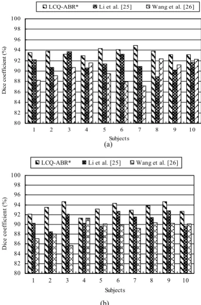
Finally, we calculate two kinds of labeling regions of longitudinal cortical surfaces. The gyri and sulci in the neonatal brain structure are two kinds of crucial organizing roles in the architectonic, connectional, and functional sense, but these organizations are not explicitly captured due to the dramatic

changes during early brain development. In this experiment, we invite six 3D-MRI experts to manually annotate the precentral gyrus (PreCG), superior temporal gyrus(STG), precentral cerebral sulci (PreCCS), and central lateral sulci (CLS) in the cortical surfaces of 10 subjects (2~10 months) according to the mean-curvature based cortical surfaces, and then we compute their manual average values of PreCG, STG, PreCCS and CLS, respectively. We further calculate the automatic labeling regions by LCQ-ABR*. We adopt the Dice coefficient [27] to quantitatively evaluate LCQ-ABR* in the segmentation performance of labeling regions of longitudinal cortical surfaces. The Dice coefficient can characterize how many pixels in the labeling region of the neonatal brain are correctly segmented and how many pixels outside the labeling region are correctly excluded, respectively. This is defined as

1 2

1 2

2

Dice coefficient 100%

 

X X

X X .

(34)

The quantitative comparisons of Dice coefficients of PreCG, STG, PreCCS, and CLS are illustrated in Fig. 9. The average Dice coefficients for PreCG/STG are 93.87%/93.89% (LCQ-ABR*), 91.97%/90.12% (Li et al.), and 91.03%/88.79%

(Wang et al.). As can be seen, LCQ-ABR* achieves the highest

Dice coefficient of gyri. Meanwhile, the average Dice coefficients for PreCCS/CLS are 92.19/94.14 (LCQ-ABR*), 89.19%/90.85% (Li et al.), and 88.66%/91.09% (Wang et al.).

It is noticed that Dice coefficients of PreCG and STG by LCQ-ABR* surpass those of PreCCS and CLS by Li et al. and

Wang et al. This shows that LCQ-ABR*also can automatically

segment and label the sulci well, and these are complementary to the cortical internal surface.

(a)

(b) 80

82 84 86 88 90 92 94 96 98 100

1 2 3 4 5 6 7 8 9 10

Subjects

D

ice co

ef

fi

ci

en

t (

%

)

LCQ-ABR* Li et al. [25] Wang et al. [26]

80 82 84 86 88 90 92 94 96 98 100

1 2 3 4 5 6 7 8 9 10

Subjects

Di

ce co

ef

fi

ci

en

t (

%

)

[image:12.595.318.525.430.744.2]