An improved emission inventory method for estimating engine exhaust emissions from ships

Original Research Article

An improved emission inventory method for estimating engine

exhaust emissions from ships

Sanaz Jahangiri

, Natalia Nikolova, Kiril Tenekedjiev

Australian Maritime College, University of Tasmania, Launceston 7250, Australia

a r t i c l e i n f o

Article history:

Received 28 November 2017 Received in revised form 1 May 2018

Accepted 10 August 2018 Available online 23 October 2018

Keywords: Shipping emissions On-board measurement Improved inventory Regression analysis

a b s t r a c t

The maritime transport industry is recognised as one of the cleanest modes of global transport. It is important to measure engine exhaust emissions to maintain its ecological superiority over road, rail, and other forms of transport.

Emission inventories are needed to estimate emissions. Current inventories need to review the emission factors (EFs) they currently employ, which generally yield over- or under-estimations. There is a need to consider more relevant measurements that will enhance the accuracy of emission prediction models. There is also a need to consider different mathematical approaches, tofind better ways to manage the many changeable parameters of fuel consumption and engine specifications used to estimate emissions.

In this study, new sets of EF equations are developed to take into consideration real-time emission measurements during 11-d emission measurements on-board of two ocean-going vessels at berth and during sailing. They were tested on two ocean-going vessels, running on slow speed diesel main engines at berth while manoeuvring and cruising. Both vessels ran on heavy diesel fuel. Regression analysis, along with a consideration of fuel consumption and engine parameters, was used to develop the equations.

The results show a better prediction of emission quantity than current inventories for different engine types, in in-port and at-sea activities, with the sum of primary emissions coming closest to the actual sea emission calculations and also to the smallest standard values. This should be helpful when upgrading environmental policies.

©2018 Chinese Institute of Environmental Engineering, Taiwan. Production and hosting by Elsevier B.V. This is an open access article under the CC BY-NC-ND license ( http://creativecommons.org/licenses/by-nc-nd/4.0/).

1. Introduction

Maritime transport is recognised as the preferred mode of global transport for goods transfer[1]. It is superior to other modes of transport such as road and rail in the large payload it can carry [2]. The globalfleet is expected to triple by 2050[3], so too will their primary emissions (NOx, SOx, CO2and CO), and it becomes impor-tant to monitor the consequent pollution.

As diesel marine fuels combust, heat energy is given out. Crude oil is the source of many of the hydrocarbon compounds which are produced during this process. Contaminants like sulphur, vana-dium, nickel, and ash are present in crude oil, and are retained

during the production of marine fuels; heavy fuel oils (HFOs) are used to contain them after intensive refining. Several factors in-fluence the quality of marine fuels: the refinery process, the crude oil quality, what kind of demands are there for the middle distillate and other residual fuels, and so on. Refinery processes often in-fluence properties and characteristics of marine fuels like specific gravity, viscosity, asphaltenes, sediment, water, _flash point, and compatibility[4].

In general, low quality fuel oil is used in the shipping industry [2]. HFO is the most common, currently used in many low-to me-dium-speed engines[5]. The sulphur content of HFO used in ships is typically 2.0e3.5%, with a global average around 2.6%[6].

There is also concern that shipping emissions are associated with adverse effects on human health, including lung cancer and heart attacks: for example, NOx, CO2and CO can result influ-like symp-toms[7], while SOxcan cause breathing issues[7]and particulate

matter (PM) may be implicated in premature deaths [8]; some

*Corresponding author.

E-mail address:[email protected](S. Jahangiri).

Peer review under responsibility of Chinese Institute of Environmental Engineering.

Contents lists available atScienceDirect

Sustainable Environment Research

-e n v i r o n m-e n t - r -e s -e a r c h /

https://doi.org/10.1016/j.serj.2018.08.005

epidemiological studies have revealed instances of asthma and heart disease[9,10]. Researchers have reported that Ocean Going Vessels account for 14e31% of global emissions of NOx, 4e9% of SOx, and 3%

of CO2, worldwide[11]. Many studies [11e13]have reviewed the impact of shipping emissions on ecology, using a variety of meth-odologies on different scales. Emissions from vessels may also have a major effect on marine boundary layers and marine productivity, as well as on ozone production and ocean acidification[14].

The importance of on-board measurement, a practical approach to measuring emissions, has been the focus of many reviews [15e21]. Most studies collecting data from slow speed diesel and medium speed diesel engines are based either on plume mea-surements or on engine test rigs[18e21], but they should also take into account on-board measurement of emission factors (EFs), which are more up-to-date and detailed, in terms of types of fuel, the regions to be studied, the characteristics of individual vessels, specifics of the engine, and activities both in-port and at-sea[22]. Moreover, they need to be more precise, and revised in terms of mathematical approaches.

Two ocean-going vessels (Vessel I and Vessel II) had their engine exhaust emissions measured in order to develop models for the emissions produced during different shipping operations. Although on-board measurement may be precise but it is not always prac-tical, as time and human resources may be limited; and it can be difficult to find vessel owners willing to install the necessary instrumentation. However, on-board measurement data were ac-quired in this study in order to develop new sets of EF equations through non-linear regression analysis, to help improve emission models and inventory calculations for different main engine types for at-sea and in-port operations.

2. Method

2.1. On-board measurement campaign

Vessel I, travelling from Port of Brisbane to Port Gladstone, un-derwent thefirst on-board measurement at a distance of 700 km; vessel II, travelling from Port Gladstone to Newcastle, underwent the second 1300 km. The routes of these vessels are presented in Fig. S1.

The ports at Brisbane, Gladstone and Newcastle, like many Australian ports, are close to urban centres, and a large percentage of the emissions from the ships, both in transit and at berth, directly affect nearby residents. As many coastal areas around the world are facing rapid and unplanned population growth, de-mographic change and development[23], there is a strong like-lihood that they, and many Australian ports, will grow to keep up with growth in shipping, and the development of a reliable method to quantify and estimate emissions will become increas-ingly important.

Procedures ISO 8178-1:2006 [24] and ISO 8178-2:2008 [25] were used to measure on-board engine exhaust. These were also used to calculate the gas-phase species emissions[24,25].Table 1 contains the engine specifications.

Fuel samples were collected from both vessels and analysed in the laboratory to determine their chemical contents. The main

chemical composition and physical properties of the HFO tested are presented inTable 2, which also indicates the percentage of sulphur present.

These results help to determine the exhaust gasflow rate, used to calculate the EFs of the vessel at various operating loads. The % mass carbon and sulphur contents are of particular interest, as they are considered the most influential when analysing the combustion process and, more importantly, the emissions generated.

Emission measurements were carried out by collecting samples using different portable instruments. Measured parameters and technical details of the applied devices are presented inTable 3 [26].

Emissions were measured and converted to weight (g). Eq.(1) gives the instantaneous emission for gaseous species, whose measurements are in ppm or percentage of gas[27]. The process used specific fuel consumption (SFOC) and formed CO2to provide the exhaust gas flow, calculated from fuel flow and air fl

ow-dbasically the sum of fuel consumption (kg h1)þair

consump-tion (kg h1). The exhaust massflow was converted into volume flow rate by using air density (at 30C air density is ~1.2 kg m3).

Emission_k¼ER_k106PV

RT MWkt (1)

where Emissionkis emissions (g), subscript k refers to emission type (NOx, SOx, CO2and CO), ER (ppm) measures gaseous species ERs,Pis average pressure of 101.3 kPa in standard conditions and a temperature of 273.1 K,V(m3h1) is calculated volumetricflow rate of the exhaust based on the available data, R (J mol1K1) is ideal gas constant, T (K) is average temperature of 273.1 K in standard conditions and an average pressure of 101.3 kPa, MW (g mol1) is molecular weight, andt(h) is recorded operation time of the vessels in different shipping modes.

The dilution ratio (DR) of each load and speed settings was then calculated. To determine the DR, CO2was used as a tracer gas. The concentration of CO2in the raw exhaust was measured directly by the Portable 5-Gas Analyser (Horiba MEXA 584L) (CO2(Raw)) and by the concentration of CO2after dilution was measured by Sable CA-10 (CO2(Diluted)); then the DR was calculated by applying Eq. (2). These calculations assume that all carbon in the fuel is completely converted to CO2[28].

DR¼ CO2ðRawÞ CO2ðBackgroundÞ

CO2ðDilutedÞ CO2ðBackgroundÞ (2)

2.2. Development of emission equations

Equations were developed applying 70% of measured ERs randomly for at berth, manoeuvring and cruising modes for each primary emission.

The regression models were based on the independent vari-ables, which in this study were data on maximum continuous rate (MCR) (asx1), shaft speed (SS) (asx2), and emissions (Y). Applying dependant variables affects the accuracy of the results. In the case

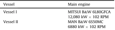
Table 1

Ships' engines specifications.

Vessel Main engine

Vessel I MITSUI B&W 6L80GFCA 12,080 kW102 RPM Vessel II MAN B&W 6S50MC

6880 kW102 RPM

Table 2

Chemical composition and physical properties of HFO.

Parameter Units Method Vessel I Vessel II

Density at 15C kg m3 _{ISO 3675 986.2 986.2} Kinetic viscosity at 50C mm2_s1 _{ISO 3140 283.0 377.0}

Carbon % mass AR 2816 88.1 88.1

Micro-carbon residue % mass ISO 10370 18.0 14.7

Sulphur % mass ISO 2719 2.9 2.8

Ash % mass ISO 6245 0.02 0.06

of this study, fuel consumption was dependent on engine load, and the base SFOC value was influenced by engine stroke type and power. Primarily, engine-model specific base values of SFOC pro-vided by the engine manufacturers were used.

Instantaneous total fuel consumption is influenced by many independent factors. The fuel consumption of main engines used in propulsion is commonly estimated as a product of the con-stant SFOC and incon-stantaneous engine power, which gives a linear relationship between fuel consumption and engine power. Ideally, all power systems that require fuel to operate should be modelled separately: the main engines for propulsion, auxiliary engines for power generation, and boilers for heat generation; however, in practice separate modelling is currently not feasible. In any case the methodologies for evaluating power and fuel consumption are fairly simple, and different assumptions were observed to provide biased estimates, especially for auxiliary engines. The SFOC effect, dependent on MCR quantities, was hidden in the developed equations; but as the objective was to analyse the variation effect of independent variables over time on final emissions, the chemical contents of the fuel (carbon, sulphur and nitrogen) were not considered as these are not time-dependant.

Table 4 shows the range of on-board measurement datasets used to develop the equations. The data on engine power, engine revolution, and other parameters including intercooled air tem-perature, scavenging air pressure and cooling fresh water were recorded every 5 s for the main engine. The only restrictions on the use of the developed EF equations would have been any datasets outside the ranges noted inTable 4for Emissions, MCR and SS, but the applied dataset roughly covered a good range for all the vari-ables mentioned in practical shipping operations.

Datafit 9 software, using different model groups including three-parameter power, three-to eleven-parameter polynomial, six

and ten Taylor series polynomial, was employed to define the models. The actual emission rates (measured instantaneously in variable timings (h) and variable engine powers (kW)) recorded every 5 s as the base for EFs in units of either ppm or %. They were then normalised to standard conditions: a temperature of 273.1 K and pressure of 101.3 kPa. Final emissions in grams were then calculated.

Having applied Datafit software, the maximum quantity of six parameters was used in this study. The equations, developed from non-linear regression analysis, are at a 95% confidence interval. The regression model's curve's alignment with the data points can be predicted by theRa2value (Eq.(3)), wherenis the number of points in the data sample andkis the number of independent regressors (the number of variables in the models excluding dependant vari-ables and constants)[29]. The adjustedR2is necessary because the value of the percentage of variation can only be explained by those independent variables that affect the dependent variables. Simply put, the adjustedR2will increase if a more useful variable is added and decrease if an un-useful (dependant) variable is added. The methodology framework is shown inFig. 1.

R2_a¼1 "

1R2ðn1Þ

nk1

#

(3)

3. Results and discussion

3.1. On-board measurement campaign

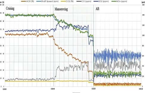
Measurements of main engine at berth were conducted when Vessel I arrived at its destination port but before the main engine were turned off. Both shaft power and SS keep changing while berthing to stop the ship making headway (Fig. 2); and both strongly affect the quantity of emissions, as depicted inFig. 2: that is, when engine speed and power suddenly undergo either positive or negative change, emissions fluctuate accordingly. Sudden change may be caused by external factors such as wind, waves or currents, or by tugs or anchors.Fig. 2shows the primary emissions, measured while the vessel was manoeuvring at the destination port. As with at-berth conditions, the levels of emissions change abruptly when SS and shaft power undergo a sudden change, often required to ensure smooth and safe berthing[30], but changes may also be caused by the geometry of the hull, the pivot point, lateral motion, the rudder, the propeller or the thrusters. The geological features of the port and under-keel clearance also affect emissions levels. Normal cruising speed was also visible for emissions (Fig. 2).

3.2. Validation of emission equations

Applying the percent-predicted method, the remaining random 30% of the emission datasets of Vessels I and II were predicted using

Table 3

Applied instrumentation specifications.

Applied devices Measured parameters Range Accuracy Flow rate (L min1₎

A Portable 5-Gas Analyser (The Horiba MEXA 584L)

HC, CO, CO2, O2and NOx(as well as monitoring airefuel equivalence ratiol)

0e60,000 ppm 0e25%

25e60 ppm 0.03e0.01%

Sable CA-10 CO2 0e5% standard

0e10% optional

1% 5e500 (103)

DMS 500 Particle size and concentration 5 nme2.5mm e 8.0

Testo 350 XL SO2, CO, CO2, O2, NO and NO2 0e10,000 ppm 0e25%

5% of mass-volume 0.8% offixed-voltage 5 ppm

1.2

Dust Trak PM1,PM2.5,PM10 0.1e10mm 5% 3.0

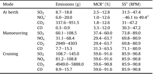
Table 4

Applied dataset range (the minimum and maximum points).

Mode Emissions (g) MCRa_{(%) SS}b_(RPM)

At berth SO2 8.7e18.8 2.5e12.8 31.5e47.4 NOxc 6.0e20.0 1.0e12.6 46.1 to 49.4d CO2 337.6e951.5 1.8e12.6 31e47.2 CO 0.3e0.9 3.3e12.0 30.3e47.2 Manoeuvring SO2 60.1e108.5 37.4e60.0 73.8e89.0 NOx 31.1e68.4 29.4e63.7 69.8e80.9 CO2 2949e4303 29.4e63.7 69.8e80.9 CO 7.7e15.3 31.3e63.5 71.1e80.9 Cruising SO2 108.7e145.0 59.6e91.6 85.9e90.8 NOx 81.2e108.8 59.6e91.6 85.9e90.8 CO2 4949.0e5888.0 59.6e90.8 85.9e90.8 CO 8.9e15.7 59.6e91.6 85.9e90.8

a_{Maximum continuous rate.} b_{Shaft speed.}

c _NOþNO 2.

d _{Negative amounts occur when the shaft churns backward to completely stop the}

the equations presented inTable S1. By comparing existing in-ventories with the actual emissions calculated using Eq.(1), it is possible to estimate primary emissions for various engine types. Our predicted inventories are closest to actual on-board estima-tions, at berth or while manoeuvring or cruising (Table S2).

The standard error of the regression or estimate value (S) (Eq. (4)) demonstrates the mathematical superiority of our predicted emission inventory over other inventories in use. The value is calculated withy0as the instantaneous calculated emission in our and other inventories andNas the total number of datasets for each primary emission of different engine types in different shipping operations. Having the smallest values, our inventories show su-periority over other inventories (Table S3).

S¼

ffiffiffiffiffiffiffiffiffiffiffiffiffiffiffiffiffiffiffiffiffiffiffiffi P

ðyy0Þ2

N

s

(4)

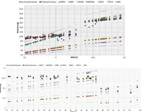
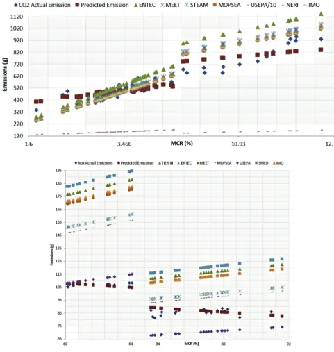
Fig. 3 presents some samples of the trends of instantaneous emissions at different MCRs, and again our predicted inventories

show the greatest affinity with on-board measurements

(Figs. S2e4). Full samples of the primary emissions in different shipping operations are presented inFigs. S2e4.

Current inventories lack detailed EF datasets for different engine types, shipping modes and emissions. As they also widely ignore national air quality programs, there is a growing need to evaluate their impact on air quality and health.

Fig. 1.The methodology framework for developing the equations.

The engine ER changes (Fig. 2) are non-linear, indicating a need to simulate emissions more practically in the mathematical model. In our study the effects of changes in engine parameters on emis-sions are considered for thefirst time.

Reasons for some non-precise estimations by each of the in-ventories are provided below:

TIER III [31] datasets do not include CO2 emissions for main engines; the effects of engine type and shipping activity not taken into account; and only limited averages of the fuel sulphur content and SFOC are considered. The data on fuel consumption are based on national data on sold fuels, not on engine fuel consumption.

Entec[27]assumes the engine EF values in different shipping activities and engine loads; and there is considerable uncertainty in some of the assumptions about engine load use in port. The quantities of fuel sulphur and carbon contents and SFOC are aver-aged, and when applying the inventory to smallerfleets, the error between the assigned EFs and thefleet value increases. Other fac-tors that may be relevant, such as how cold-started engines or various engine loads affect performance in the course of manoeu-vring, are ignored.

Methodology for Emissions and Energy consumption for Transport (MEET)[32]calculates averaged fuel consumption and engine loads for engines rather than addressing specific situations

that may affect performance: for instance, the same EF is used for CO engines at berth and manoeuvring; and for the CO engines of slow- and medium-speed diesel engines. It does not consider the effect of using different marine fuels in engine NOxEFs in different

shipping operations.

Ship Traffic Emission Assessment Model [33]datasets do not include CO emissions. As a requirement of the SOxEmission Control

Area regulations of the International Maritime Organisation (IMO), only a sulphur mass-percentage of 1.5 is assumed and modelled for main engines. Different engine specifications or shipping opera-tions are not considered when assigning engine NOxEFs. Engine

loads can often influence EFs: for instance, engines operating under a low load may have higher emissions, particularly during harbour manoeuvring; such variations in EFs as a function of engine load are not taken into account.

Monitoring programme on air pollution from sea-going vessels (MOPSEA)'s[34]activity data are gathered from information sys-tems not designed for inventory emissions, so it takes time and experience to repurpose the data to suit them to the emission model, and the work needs to be simplified and tailored to befit for inventory purposes. This model too makes various assumptions about fuel use and the percentage of MCR which do not reflect these parameters in practice: for example, averaged engine EFs per

ship type are used instead of specificfigures. There is inadequate focus on engine loads during different shipping activities, and no coverage of engine load variations over 85% or under 10% in NOx

and CO EFs. Nor is there adequate direction for dealing with missing data, or for implementing and using Automatic Identification Sys-tem (AIS) data.

National Environmental Research Institute (NERI)[35]uses the same CO EFs without consideration of engine type or shipping ac-tivity; nor are consistent emission data available as a function of the engine age. In addition, country-specific EFs for CO2do not consider engine types or shipping activities.

United States Environmental Protection Agency (USEPA)'s[36] basis for its operating data seems to have various assumptions that are not validated by the Energy and Environmental Analysis as their contractor. It categorises engines by individual cylinder displacement, which may not indicate a true relationship with high, medium, and slow speeds. Large inconsistencies appear be-tween the output given at full load and the actual ratings of the engine, pointed out in Lloyd's analysis.

The data analysis is mostly carried out on engines with a rating of less than 8000 kW, and the applicability of the EFs obtained to engines of all sizes is debatable. There is no consistency between

engines' rated power and testing conditions, so EPA categories cannot be determined. There is no agreement on the actual numbers or types of engine, and no reporting of engine markers or displacements. In some instances, the reported maximum power and engine ratings show discrepancies.

The Environment Canada report defines the three modes and engine load factor variations under which its engines were tested, and does not consider the extent of variation that may exist be-tween engines in the same category;‘normal cruise’and‘docking operation’conditions are undefined in the procedures of the BC Ferry Test Program. Engine NOx and CO have the same EFs,

regardless of fuel or engine used or consideration of shipping activity.

Swedish Methodology for Environmental Data [37]inventory likewise Entec[27], mentioned in above paragraphs, suffers from non-precise EFs. Also, there is a great deal of uncertainty about ‘manoeuvring’ (the assumption is that engines operate at 20% MCR), as well as the need for manoeuvring emissions to take into consideration that emissions from cold state engines, especially CO emissions, which would be significantly different than those from warmer engines. Variability of emissions can also be caused by rapid changes to load during manoeuvring: this study takes none of these into account.

Engine EFs (derived from steady state loads of 70e100%) are

multiplied‘at sea’by 0.8 for NOxand by 2.0 for CO for all engines

running on diesel. This means that there is significant uncertainty regarding the results. Emission estimations for engines at berth are not considered. The estimates of the fuel sulphur in various fuels over the years are unspecified, and it is assumed that between 1990 and 2003, fuel-dependent EFs of CO2were constant. Considering that EFs are different and there is anticipated uncertainty, speci-fying exactly how biased emission estimations can be, especially when only at-sea EFs are at play, is difficult.

IMO[38]bases its SOxbase line EFs on a 2.7% sulphur content

HMO, although the world average of fuel sulphur is in constant change. The effect of using different fuel types is not considered in applying base SFOC values to engines; the parabolic SFOC de-pendency on engine load is not considered in HFO; and transient engine load changes are not considered in CO EFs.

There are uncertainties about how many active ships exist, and which are allocated to domestic or international voyages. Currently discrepancies occur between the number of active ships described by the IHSF and those observed on AIS, although this will reduce slightly as the availability of AIS data improves. The bottom-up method is used when location information is available, but AIS coverage is not so consistently high for the voyage-by-voyage de-tails to be identified either. Some uncertainties may also arise if the ship is not visible on AIS and its speed is estimated.

4. Conclusions

The non-linear regression analysis used here to develop new sets of EF equations on each primary emission for engines at berth, manoeuvring, and at sea predicts emissions more accurately than current inventories. The sampling will help in developing emission models and inventory calculations that can be used to outline MCR, SS, and emission datasets more effectively than is currently achieved.

Acknowledgements

Special thanks to National Centre for Maritime Engineering and Hydrodynamic in Australian Maritime College and Queensland University of Technology for their support of this study. The

generous cooperation of Port of Brisbane Corporation is

acknowledged, as are Maritime Safety Queensland and stevedore operators AAT, Patricks and DP World.

Appendix A. Supplementary data

Supplementary data to this article can be found online at https://doi.org/10.1016/j.serj.2018.08.005.

References

[1] Wang C, Corbett JJ, Firestone J. Improving spatial representation of global ship emissions inventories. Environ Sci Technol 2008;42:193e9.

[2] Deniz C, Kilic A. Estimation and assessment of shipping emissions in the re-gion of Ambarli Port, Turkey. Environ Prog Sustain Energy 2010;29:107e15. [3] Eyring V, K€ohler HW, van Aardenne J, Lauer A. Emissions from international

shipping: 1. The last 50 years. J Geophys Res Atmos 2005;110:1e12. [4] ABS. Notes on Heavy Fuel Oil. Houston, TX: American Bureau of Shipping; 1984. [5] Goldsworthy L, Galbally IE. Ship engine exhaust emissions in waters around

Australiaean overview. Air Qual Clim Change 2011;45:24e32.

[6] IMO. Report of the Marine Environment Protection Committee on its Sixty-first Session. London, UK: International Maritime Organisation; 2010. [7] Fournier A. Controlling Air Emissions from Marine Vessels: Problems and

Opportunities. Santa Barbara, CA: University of California Santa Barbara; 2006. [8] USEPA. Control of Emissions from New Marine Compression-ignition Engines at or Above 30 Litres Per Cylinder. Washington, DC: US Environmental Pro-tection Agency; 2010.

[9] Kim S, Hwang JW, Lee CS. Experiments and modeling on droplet motion and atomization of diesel and bio-diesel fuels in a cross-flowed air stream. Int J Heat Fluid Flow 2010;31:667e79.

[10] Lu G, Brook JR, Alfarra MR, Anlauf K, Leaitch WR, Sharma S, et al. Identification and characterization of inland ship plumes over Vancouver, BC. Atmos Envi-ron 2006;40:2767e82.

[11] Kilic A, Deniz C. Inventory of shipping emissions in Izmit Gulf, Turkey. Environ Prog Sustain Energy 2010;29:221e32.

[12] Moreno-Gutierrez J, Calderay F, Saborido N, Boile M, Valero RR, Duran-Grados V. Methodologies for estimating shipping emissions and energy con-sumption: a comparative analysis of current methods. Energy 2015;86: 603e16.

[13] Merk O. Shipping Emissions in Ports. Paris, France: Organisation for Economic Co-operation and Development; 2014.

[14] Hassellov IM, Turner DR, Lauer A, Corbett JJ. Shipping contributes to ocean acidification. Geophys Res Lett 2013;40:2731e6.

[15] Cooper DA, Peterson K, Simpson D. Hydrocarbon, PAH and PCB emissions from ferries: a case study in the SkagerrakeKattegateOresund region. Atmos

Environ 1996;30:2463e73.

[16] Cooper DA, Andreasson K. Predictive NOxemission monitoring on board a

passenger ferry. Atmos Environ 1999;33:4637e50.

[17] Cooper DA. Exhaust emissions from high speed passenger ferries. Atmos Environ 2001;35:4189e200.

[18] Lyyranen J, Jokiniemi J, Kauppinen EI, Joutsensaari J. Aerosol characterisation in medium-speed diesel engines operating with heavy fuel oils. J Aerosol Sci 1999;30:771e84.

[19] Petzold A, Hasselbach J, Lauer P, Baumann R, Franke K, Gurk C, et al. Experi-mental studies on particle emissions from cruising ship, their characteristic properties, transformation and atmospheric lifetime in the marine boundary layer. Atmos Chem Phys 2008;8:2387e403.

[20] LRES. Marine Exhaust Emissions Research Programme: Steady State Opera-tion. London, UK: Lloyd's Register Engineering Services; 1990.

[21] Corbett JJ, Koehler HW. Updated emissions from ocean shipping. J Geophys Res Atmos 2003;108:4650.

[22] Jahangiri S, Kam US, Garaniya V, Abbassi R, Enshaei H, Brown RJ, et al. Development of Emission Factors for Ships' Emissions at Berth. Australasian Coasts&Ports. Barton, Australia: Engineers Australia; 2017. p. 646e52. [23] Satumanatpan S, Chuenpagdee R. Assessing governability of environmental

protected areas in Phetchaburi and Prachuap Khiri Khan, Thailand. Marit Stud 2015;14:1e19.

[24] ISO. ISO 8178-1. Reciprocating Internal Combustion Engines e Exhaust

Emission Measuremente Part 1: Test-bed Measurement of Gaseous and

Particulate Exhaust Emissions. Geneva, Switzerland: International Organiza-tion for StandardizaOrganiza-tion; 2006.

[25] ISO. ISO 8178-2. Reciprocating Internal Combustion Engines e Exhaust

Emission MeasurementePart 2: Measurement of Gaseous and Particulate

Exhaust Emissions under Field Conditions. Geneva, Switzerland: International Organization for Standardization; 2008.

[26] Australian Maritime College. Development of a Methodology to Measure and Assess Ship Emissions. Tokyo, Japan: International Association of Maritime Universities; 2016.

[27] Whall C, Scarbrough T, Stavrakaki A, Green C, Squire J, Noden R. UK Ship Emissions Inventory. London, UK: Entec UK Limited; 2010.

[29] Harel O. The estimation of R2and adjusted R2in incomplete data sets using multiple imputation. J Appl Stat 2009;36:1109e18.

[30] Fu ML, Ding Y, Ge YS, Yu LX, Yin H, Ye WT, et al. Real-world emissions of inland ships on the Grand Canal, China. Atmos Environ 2013;81: 222e9.

[31] Trozzi C, De Lauretis R, Rypdal K, Webster A, Fridell E, Reynolds G, et al. In-ternational navigation, national navigation, national fishing and military (shipping). In: EMEP/EEA Air Pollutant Emission Inventory Guidebook. Luxembourg: European Environment Agency; 2013.

[32] TRL. Methodology for Calculating Transport Emissions and Energy Con-sumption. Crowthorne, UK: Transport Research Laboratory; 1999.

[33] Jalkanen JP, Brink A, Kalli J, Pettersson H, Kukkonen J, Stipa T. A modelling system for the exhaust emissions of marine traffic and its application in the Baltic Sea area. Atmos Chem Phys 2009;9:9209e23.

[34] Gommers A, Verbeeck L, Van Cleemput E, Schrooten L, De Vlieger I. Moni-toring Programme on Air Pollution from SEA-going Vessels EV/43, Pt 2. Brussels, Belgium: Belgian Science Policy; 2007. http://www.belspo.be/ belspo/organisation/publ/pub_ostc/EV/rappEV43_en.pdf.

[35] Olesen HR, Winther M, Ellermann T, Christensen J, Plejdrup M. Ship Emissions and Air Pollution in Denmark. Copenhagen, Denmark: Danish Environmental Protection Agency; 2009.

[36] USEPA. Analysis of Commercial Marine Vessels Emissions and Fuel Con-sumption Data. Washington, DC: US Environmental Protection Agency; 2000. [37] Cooper D, Gustafsson T. Methodology for Calculating Emissions from Ships: 1. Update of Emission Factors. Norrkoping, Sweden: Swedish Meteorological and€ Hydrological Institute; 2004.